Open book decompositions of fibre sums in contact topology

Abstract.

In the present paper we describe compatible open books for the fibre connected sum along binding components of open books, as well as for the fibre connected sum along multi-sections of open books. As an application the first description provides simple ways of constructing open books supporting all tight contact structures on $T^{3}$, recovering a result by van Horn-Morris, as well as an open book supporting the result of a Lutz twist along a binding component of an open book, recovering a result by Ozbagci–Pamuk.

Introduction

According to a theorem of Alexander [Ale-SystemsOfKnottedCurves] every closed oriented $3$-manifold admits a so-called open book decomposition. While it had been known for almost 40 years that open books carry a natural contact structure [MR0375366], at the beginning of the millennium it turned out that this was just one fragment of a much deeper correlation. As was observed by Giroux [MR1957051], contact structures in dimension $3$ are of purely topological nature: he established a one-to-one correspondence between isotopy classes of contact structures and open book decompositions up to positive stabilisation. Ever since it is of interest to recover properties and constructions of contact structures in the language of open books.

In the present paper we approach how the contsruction of the fibre connected sum affects an underlying open book structure of the original manifold under certain assumptions. Fibre connected sums in the contact setting recently drew some attention appearing in Wendl’s [2010arXiv1009.2746W] notion of planar torsion, an obstruction for strong fillability generalising overtwistedness and Giroux torsion. In essence, a contact manifold admits planar torsion if it can be written as the binding sum, i.e. the fibre connected sum along binding components of an open book, of a non-trivial ($\geq 2$) number of open books, one of which has planar pages.

The present paper, suppressing the preliminaries, splits into two parts, §2 and §3, which can be read independently. The main results are descriptions of compatible open books for:

• The fibre connected sum along binding components of open books – cf. Theorem 3 on page 3.

• The fibre connected sum along multi-sections of open books – cf. Theorem 7 on page 7.

As an application the first description provides simple ways of constructing open books supporting all tight contact structures on $T^{3}$, recovering a result by van Horn-Morris [vanHornMorris-Thesis], as well as an open book supporting the result of a Lutz twist along a binding component of an open book, recovering a result by Ozbagci–Pamuk [2009arXiv0905.0986O].

Acknowledgements

The results presented in this paper are part of my thesis [Klukas-Thesis]. I want to thank my advisor Hansjörg Geiges for introducing me to the world of contact topology and for all the helpful discussions, especially for initializing the first part of the present paper. I deeply thank John Etnyre for many inspiring conversations and, in particular, for initializing the second part of this paper.

The research for the second part of this paper took place during a research visit at the Georgia Institute of Technology, Atlanta GA, USA, under the supervision of John Etnyre. I want to thank GaTech and John Etnyre for their hospitality. This research visit was additionally supported by the DAAD (German Academic Exchange Service). Overall the author was supported by the DFG (German Research Foundation) as fellow of the graduate training programm Global structures in geometry and analysis at the Mathematics Department of the University of Cologne, Germany.

1. Preliminaries

1.1. Open books

An open book decomposition of a $3$-dimensional manifold $M$ is a pair $(B,\pi)$, where $B$ is a disjoint collection of embedded circles, in $M$, called the binding of the open book and $\pi\colon\thinspace M\setminus B\to S^{1}$ is a (smooth, locally trivial) fibration such that each fibre $\pi^{-1}(\varphi)$, $\varphi\in S^{1}$, corresponds to the interior of a compact hypersurface $\Sigma_{\varphi}\subset M$ with $\partial\Sigma_{\varphi}=B$. The hypersurfaces $\Sigma_{\varphi}$, $\varphi\in S^{1}$, are called the pages of the open book.

In some cases we are not interested in the exact position of the binding or the pages of an open book decompositon inside the ambient space. Therefore, given an open book decomposition $(B,\pi)$ of a $3$-manifold $M$, we could ask for the relevant data to remodel the ambient space $M$ and its underlying open books structure $(B,\pi)$, say up to diffemorphism. This leads us to the following notion.

An abstract open books is a pair $(\Sigma,\phi)$, where $\Sigma$ is a compact surface with non-empty boundary $\partial\Sigma$, called the page and $\phi\colon\thinspace\thinspace\Sigma\to\Sigma$ is a diffeomorphism equal to the identity near $\partial\Sigma$, called the monodromy of the open book. Let $\Sigma(\phi)$ denote the mapping torus of $\phi$, that is, the quotient space obtained from $\Sigma\times[0,1]$ by identifying $(x,1)$ with $(\phi(x),0)$ for each $x\in\Sigma$. Then the pair $(\Sigma,\phi)$ determines a closed manifold $M_{(\Sigma,\phi)}$ defined by

(1) $$M_{(\Sigma,\phi)}:=\Sigma(\phi)\cup_{\mbox{\rm id}}(\partial\Sigma\times D^{2}),$$

where we identify $\partial\Sigma(\phi)=\partial\Sigma\times S^{1}$ with $\partial(\partial\Sigma\times D^{2})$ using the identity map. Let $B\subset M_{(\Sigma,\phi)}$ denote the embedded link $\partial\Sigma\times\{0\}$. Then we can define a fibration $\pi\colon\thinspace M_{(\Sigma,\phi)}\setminus B\to S^{1}$ by

$$\left.\begin{array}[]{l}[x,\varphi]\\ [\theta,r\mathrm{e}^{i\pi\varphi}]\end{array}\right\}\mapsto[\varphi],$$

where we understand $M_{(\Sigma,\phi)}\setminus B$ as decomposed in (1) and $[x,\varphi]\in\Sigma(\phi)$ or $[\theta,r\mathrm{e}^{i\pi\varphi}]\in\partial\Sigma\times D^{2}\subset\partial\Sigma\times\mathbb{C}$ respectively. Clearly $(B,\pi)$ defines an open book decomposition of $M_{(\Sigma,\phi)}$.

On the other hand, an open book decomposition $(B,\pi)$ of some $3$-manifold $M$ defines an abstract open book as follows: identify a neighbourhood of $B$ with $B\times D^{2}$ such that $B=B\times\{0\}$ and such that the fibration on this neighbourhood is given by the angular coordinate, $\varphi$ say, on the $D^{2}$-factor. We can define a $1$-form $\alpha$ on the complement $M\setminus(B\times D^{2})$ by pulling back $d\varphi$ under the fibration $\pi$, where this time we understand $\varphi$ as the coordinate on the target space of $\pi$. The vector field $\partial\varphi$ on $\partial\big{(}M\setminus(B\times D^{2})\big{)}$ extends to a nowhere vanishing vector field $X$ which we normalise by demanding it to satisfy $\alpha(X)=1$. Let $\phi$ denote the time-$1$ map of the flow of $X$. Then the pair $(\Sigma,\phi)$, with $\Sigma=\overline{\pi^{-1}(0)}$, defines an abstract open book such that $M_{(\Sigma,\phi)}$ is diffeomorphic to $M$.

1.1.1. Examples

Understand $S^{3}$ as the unit sphere in $\mathbb{C}^{2}$, i.e. as the subset of $\mathbb{C}^{2}$ given by

$$S^{3}=\{(z_{1},z_{2})\in\mathbb{C}^{2}\colon\thinspace|z_{1}|^{2}+|z_{2}|^{2}=1\}.$$

We give three examples of open book decompositions of $S^{3}$:

• Set $B=\{(z_{1},z_{2})\in S^{3}\colon\thinspace z_{1}=0\}$. Note that $B$ is an unknotted circle in $S^{3}$. Consider the fibration

  $$\pi\colon\thinspace S^{3}\setminus B\to S^{1}\subset\mathbb{C},\ (z_{1},z_{2})\mapsto\frac{z_{1}}{|z_{1}|}.$$

  In polar coordinates this map is given by $(r_{1}\mathrm{e}^{i\varphi_{1}},r_{2}\mathrm{e}^{i\varphi_{2}})\mapsto\varphi_{1}$. Observe that $(B,\pi)$ defines an open book decomposition of $S^{3}$ with pages diffeomorphic to $D^{2}$ and trivial monodromy.

• Set $B_{+}=\{(z_{1},z_{2})\in S^{3}\colon\thinspace z_{1}z_{2}=0\}$. Observe that $B_{+}$ describes the positive Hopf link. Consider the fibration

  $$\pi_{+}\colon\thinspace S^{3}\setminus B_{+}\to S^{1}\subset\mathbb{C},\ (z_{1},z_{2})\mapsto\frac{z_{1}z_{2}}{|z_{1}z_{2}|}.$$

  One can show that $(\pi_{+},B_{+})$ defines an open book decomposition of $S^{3}$ with annular pages and monodromy given by a left-handed Dehn twist along the core of the annulus.

• Set $B_{-}=\{(z_{1},z_{2})\in S^{3}\colon\thinspace z_{1}\overline{z_{2}}=0\}$. Observe that $B_{-}$ describes the negative Hopf link. Consider the fibration

  $$\pi_{-}\colon\thinspace S^{3}\setminus B_{-}\to S^{1}\subset\mathbb{C},\ (z_{1},z_{2})\mapsto\frac{z_{1}\overline{z_{2}}}{|z_{1}\overline{z_{2}}|}.$$

  One can show that $(\pi_{+},B_{+})$ defines an open book decomposition of $S^{3}$ with annular pages and monodromy given by a right-handed Dehn twist along the core of the annulus.

1.2. Stabilisations of open books

Let $\Sigma$ be a compact surface with non-empty boundary and $\phi\colon\thinspace\Sigma\to\Sigma$ a diffeomorphism equal to the identity near $\partial\Sigma$. Suppose further we are given a properly embedded arc $a\subset\Sigma$. The positive (negative) stabilisation of the abstract open book $(\Sigma,\phi)$ is the abstract open book obtained by adding a $1$-handle to the original page $\Sigma$ along the endpoints of $a$, and changing the monodromy by composing it with a right- (left-) handed Dehn twist along the simple closed curve obtained by the union of $a$ and the core of the $1$-handle. The open books described in parts (2) and (3) of the preceding example are instances of a positive and negative stabilisation respectively of the open book described in the first part.

A positive and negative stabilisation respectively can be understood as a suitable connected sum with the open book described in part (2) or part (3) of the preceding example. This viewpoint will draw more attention once we introduced the interplay of open books and contact structures, cf. §1.3 below. To be more precise: a positive stabilisation of an open book does not change the underlying contact structure, whereas a negative stabilisation turns it into an overtwisted one.

1.3. Compatibility

A positive contact structure $\xi=\ker\alpha$ and an open book decomposition $(B,\pi)$ of $M$ are said to be compatible with each other, if the $2$-form $d\alpha$ induces a symplectic form on each page, defining its positive orientation, and the $1$-form $\alpha$ induces a positive contact form on $B$.

In dimension equal to $3$ it can be shown that any two contact structures supported by the same open book decomposition are in fact contact isotopic (cf. [MR2249250]). The open books described in parts (1) and (2) of Example 1.1.1 above support the standard contact structure $\xi_{st}$ on $S^{3}$, whereas part (3) supports the overtwisted contact structure $\xi_{1}$ which is obtained by a Lutz twist along a transverse unknot $U\subset(S^{3},\xi_{st})$ with self-linking number $-1$.

1.4. The fibre connected sum

Let $K\subset(M,\xi)$ be a positive transverse knot sitting in a contact $3$-manifold $(M,\xi)$. We may identify a neighbourhood of $K$ with an $\varepsilon$-neighbourhood $N_{\varepsilon}\subset S^{1}\times\mathbb{R}^{2}$, where $K=S^{1}\times\{0\}$. Then, with $S^{1}$-coordinate $\theta$, polar coordinates $(r,\varphi)$ on $\mathbb{R}^{2}$, and for a suitable $\varepsilon>0$, the contact structure

$$d\theta+r^{2}\thinspace d\varphi=0$$

provides a model for the above neighbourhood of $K$. Let $M_{K}=M\setminus N_{\delta}$ denote the complement of a $\delta$-neighbourhood $N_{\delta}\subset N_{\varepsilon}$, with $0<\delta<\varepsilon$, where we change the contact structure as follows. Replace the contact structure $\xi$ over $N_{\varepsilon}\setminus N_{\delta}$ by the kernel of the contact $1$-form $d\theta+f(r)\thinspace d\varphi$, where $f:[\delta,\infty]\to\mathbb{R}$ is a function that equals $r^{2}$ away from $\delta$, satisfies $f^{\prime}>0$, $f^{\prime}(\delta)=1$ and $f(\delta)=0$. We will refer to $M_{K}$ as obtained by blowing up $K$. The inverse operation of blowing up will be referred to as collapsing.

Suppose now we are given a pair of positive transverse knots $K_{0},K_{1}\subset(M,\xi)$ wich are endowed with a framing. Let $M_{K_{0},K_{1}}$ denote the result of blowing up each of the knots $K_{0}$ and $K_{1}$. Each of the boundary tori associated to $K_{0}$ and $K_{1}$ respectively admits a natural identification with $\mathbb{R}^{2}/\mathbb{Z}^{2}$ by sending the meridian to the the $x$-axis and the framing-direction to the $y$-axis. The fibre connected sum $\#_{K_{0},K_{1}}(M,\xi)$ is the closed oriented manifold given as the quotient space

$$\#_{K_{0},K_{1}}(M,\xi):=(M_{K_{0},K_{1}})/\sim$$

where we identify the boundary tori with respect to the gluing map sending $(x,y)$ to $(-x,y)$.

2. An open book supporting the binding sum

In the previous section we introduced the fibre connected sum along a pair of positively transverse knots in a contact manifold. In the present section we proceed by considering two special cases, the fibre connected sum along binding components of open books and the fibre connected sum along sections of open books. Throughout the whole section let $(M,\xi)$ be a closed, not necessarily connected, contact $3$-manifold supported by an open book $(\Sigma,\phi)$. Let $B\subset M$ denote the embedded binding of the open book.

Suppose we have chosen the transverse knots $K_{0}$ and $K_{1}$ to be components of the binding of the open book decomposition $(\Sigma,\phi)$. Since the pages induce a natural framing for $K_{0}$ and $K_{1}$ respectively we can think of it as the zero-framing and hence can measure all other trivialisations relative to it. Note that performing the fibre connected sum with framings $m_{1},m_{2}\in\mathbb{Z}$ equals the the result of performing the fibre connected sum with framings $\widetilde{m}_{1}=m_{1}+m_{2}$ and $\widetilde{m}_{2}=0$. So in the following we just fix one framing assuming the other one to be zero. The result of performing the fibre connected sum along two binding components $K_{0}$ and $K_{0}$ with framing $m\in\mathbb{Z}$ will be referred to as binding sum along $K_{0}$ and $K_{1}$ and will be denoted by

$$\boxplus_{m}(\Sigma,\phi).$$

Now suppose $K_{0}$ and $K_{1}$ are positive transverse knots intersecting every page transversely and exactly once. We will refer to such a knot as a section of the open book, since it induces a section of the fibration $M\setminus B\to S^{1}$. Again understand these knots as endowed with a framing. By nature of the sections we can embed the normal bundle $N_{i}$, $i=0,1$, such that each fibre corresponds to a disc neighbourhood $D_{i}\subset\Sigma$ of the intersection point $\{p_{i}\}=K_{i}\cap\Sigma$. In the following we will see that fibre connected sums of this kind are nicely adapted to the underlying open book decomposition.

The new fibre is obtained by replacing $D_{0}\cup D_{1}$ by $[-1,1]\times S^{1}$. However, the change of monodromy is less obvious. To see how the monodromy changes, consider a vector field transverse to the fibres in $M$ with $K_{0}$ and $K_{1}$ as closed orbits such that the return map $h$ on a fibre $\Sigma$ fixes a disc neighbourhood $D_{i}$ of each $\Sigma\cap K_{i}$ and such that closed orbits close to $K_{0}$ and $K_{1}$ represent the trivialisations of the sections. The new monodromy is equal to $h$ on $\Sigma\setminus(D_{0}\cup D_{1})$ and the identity on $[-1,1]\times S^{1}$.

For our purposes it will be sufficient just to consider trivial sections, that is, sections corresponding to a single fix point $p\in\Sigma$ of the monodromy of a given abstract open book $(\Sigma,\phi)$. In this case we obtain natural trivialisations of the normal bundles given by a parallel copy of the knot corresponding to a nearby point. Furthermore we can assume the given monodromy $\phi$ to be the identity on $D_{0}\cup D_{1}$. So by the observations above, the new monodromy will be given by $\phi$ on $\Sigma\setminus(D_{0}\cup D_{1})$ and the identity on $[0,1]\times S^{1}$.

Lemma 1.

Let $K$ be a section of an open book $(B,\pi)$ supporting a contact $3$-manifold $(M,\xi)$. Then there is another contact structure $\xi^{\prime}$ which is still supported by $(B,\pi)$ and such that the intersection point of $K$ and any page $\Sigma_{\varphi}$, $\varphi\in S^{1}$, corresponds to an elliptic singularity of the characteristic foliation $(\Sigma_{\varphi})_{\xi^{\prime}}$. The analogous statement holds for multi-sections of open books as defined in Section 3.

Proof.

Fix a page $\Sigma=\Sigma_{0}$ of $(B,\pi)$ and let $N(B)$ denote a neighbourhood of the binding disjoint from $K$. Furthermore let $p=\Sigma\cap K$ denote the transverse intersecion of $K$ and $\Sigma$. Identify the complement $M\setminus N(B)$ of $N(B)$ with the mapping torus $\Sigma(\phi)$ of a suitable monodromy map $\phi\colon\thinspace\Sigma\to\Sigma$, i.e. we have

$$M\setminus N(B)\cong\Sigma\times[0,1]/\sim,$$

where we identify $(x,1)$ with $(\phi(x),1)$ for all $x\in\Sigma$. Note that we may assume that we have chosen $\phi$ in such a way that, with respect to the above identification, $\{p\}\times[0,1]$ descends to $K$. Moreover we can assume $\phi$ to fix a little neighbourhood of $p$. Hence it remains to show that there is a contact structure on $\Sigma(\phi)$ satisfying the desired property for this particular case. Following the construction of Thurston and Winkelnkemper [MR0375366] all we have to do is choose an exact volume form $d\beta$ on $\Sigma$ such that its dual vector field $Y$ points outwards along $\partial\Sigma$ and has an elliptic singularity at $p$. ∎

Lemma 2.

The contact manifold resulting from the (contact) fibre connected sum along a section of an open book is compatible with the corresponding open book. The analogous statement holds for multi-sections of open books as defined in Section 3.

Proof.

According to Lemma 1 We can assume, by applying an isotopy of $\xi$, that the intersections of $K_{i}$ with the pages $\Sigma_{\theta}$ correspond to elliptic singularities of the characteristic foliation $(\Sigma_{\theta})_{\xi}$. If we perform the fibre connected sum, the resulting contact structure $\xi^{\prime}$ and the open book $(\Sigma^{\prime},\phi^{\prime})$ are related as follows. As observed in the above discussion the new fibre $\Sigma^{\prime}$ is obtained by replacing $D_{0}\cup D_{1}\subset\Sigma$ by $[-1,1]\times S^{1}$. Since the origin $0\in D_{i}$ corresponds to an elliptic singularity of the characteristic foliation $(D_{i})_{\xi}$ it gives rise to a closed leaf in the characteristic foliation $([-1,1]\times S^{1})_{\xi^{\prime}}$ corresponding to the core $\{0\}\times S^{1}$ of the annulus. Outside this curve the characteristic foliation agrees with the foliations on $D_{i}\setminus\{0\}$.

The new contact structure $\xi^{\prime}$ can be isotoped to be arbitrarily close (as oriented plane fields), on compact subsets of the pages, to the tangent planes to the pages of the open book in such a way, that after some point in the isotopy the contact planes are transverse to $B^{\prime}$ and transverse to the pages of the open book in a fixed neighbourhood of $B^{\prime}$ (because this holds for the original open book $(\Sigma,\phi)$). Hence, according to [MR2249250]*Lemma 3.5, the contact structure $\xi^{\prime}$ is supported by the open book $(\Sigma^{\prime},\phi^{\prime})$. ∎

Remark.

An open book decomposition can be understood as the boundary of an achiral Lefschetz fibration. In a similar fashion the fibre sum along sections corresponds to the boundary of a broken achiral Lefschetz fibration, see [MR2350472] for reference.

Given a simple closed curve $\alpha$ on some surface $\Sigma$ we denote by $\tau_{\alpha}$ and $(\tau_{\alpha})^{-1}$ respectively the right- and left-handed Dehn twist along $\alpha$. When we deal with the concatenation of Dehn twists we sometimes omit the concatenation symbol “$\circ$” to simplify the notation. In this fashion it makes sense to consider $n$th-powers $(\tau_{\alpha})^{n}$ of Dehn twists, where the zero power $(\tau_{\alpha})^{0}$ is defined to be the identity map.

Let $K\subset\partial\Sigma$ denote a boundary component of the page $\Sigma$ provided with some framing $m\in\mathbb{Z}$ and let $K^{\prime}\subset\Sigma$ denote the transverse knot indicated by the black dot in Figure 1 which we understand $K^{\prime}$ as zero-framed. The framings are understood as measured with respect to their respective natural zero-framings as explained above.

Definition 1.

We will refer to $(K,m)$ as admitting a navel if the monodromy near the boundary component is given by $\tau_{\alpha}\tau_{\beta}^{-1}\tau_{\gamma}^{m-1}$, where the curves $\alpha,\beta,\gamma\subset\Sigma$ are given as in Figure 1. The transverse knot $K^{\prime}=(K^{\prime},0)$ indicated by the black dot in Figure 1 will be referred to as core of the navel corresponding to $(K,m)$.

Observe that we can change every boundary component into a navel, since the monodromy $\tau_{\alpha}\tau_{\beta}^{-1}\tau_{\gamma}^{m-1}$ is isotopic to the identity. In the following proposition we will express the binding sum as the fibre sum along the core of its corresponding navel.

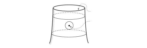
Figure 1. Binding component admitting a navel.

Theorem 3.

Let $K\subset\partial\Sigma$ be a binding component provided with a framing $m\in\mathbb{Z}$. Then the framed knot $(K,m)$ is transversely isotopic to the corresponding core $(K^{\prime},0)$ of its navel. In consequence the result of performing the binding sum with framing $m\in\mathbb{Z}$ along two binding components $K_{0},K_{1}\subset\Sigma$ corresponds to the fibre sum along the cores $K^{\prime}_{0},K^{\prime}_{1}$ of their corresponding navels (cf. also Figure 2).

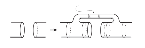
Figure 2. An open book supporting the binding sum.

Proof.

Identify a neighbourhood of the binding component $K\subset\partial\Sigma$ with an $\varepsilon$-neighbourhood $N_{\varepsilon}\subset S^{1}\times\mathbb{R}^{2}$, where $K=S^{1}\times\{0\}$. Then, with $S^{1}$-coordinate $\theta$, polar coordinates $(r,\varphi)$ on $\mathbb{R}^{2}$, and for a suitable $\varepsilon>0$, the contact structure

$$d\theta+r^{2}\thinspace d\varphi=0$$

provides a model for the above neighbourhood of $K$. Moreover we can assume that over this neighbourhood the pages are given by the preimages of the projection on the angular-coordinate $\varphi$, i.e. the closure of every page can be described as $A_{\varphi}=S^{1}\times[0,\varepsilon]\times\{\varphi\}$ for some appropriate $\varphi\in S^{1}$.

We will now apply the first part $\tau_{\alpha}\tau_{\beta}^{-1}$ of the monodromy of the navel (the twists $\tau_{\gamma}^{m-1}$ just take care of the framings, but we will come to that later). Let $S^{1}\times[\delta,\varepsilon]\times S^{1}$ denote the complement of a $\delta$-neighbourhood $N_{\delta}$ of $K$ in $N_{\varepsilon}$ for some small $0<\delta<\varepsilon$. Consider the map $\phi\colon\thinspace S^{1}\times[\delta,\varepsilon]\to S^{1}\times[\delta,\varepsilon]$ defined by

$$\phi(\theta,r):=(\theta+\thinspace h(r),r),$$

where $h:[\delta,\varepsilon]\to[0,1]$ is the function satisfying the following properties:

• $h(r)=0$ for $r$ near $\delta$ and near $\varepsilon$,

• $h(r)=1$ on an interval containing $\frac{\varepsilon+\delta}{2}$,

• $h^{\prime}(r)\geq 0$ for $r<\frac{\varepsilon+\delta}{2}$ and

• $h^{\prime}(r)\leq 0$ for $r>\frac{\varepsilon+\delta}{2}$.

Note that with respect to the identification $S^{1}\equiv\mathbb{R}/\mathbb{Z}$ the map $\phi$ is indeed well-defined and observe that $\phi$ equals $\tau_{\alpha}\tau_{\beta}^{-1}$ and is isotopic to the identity. Consider the corresponding mapping torus $A(\phi)$, that is

$$A(\phi)=\big{(}S^{1}\times[\delta,\varepsilon]\times[0,1]\big{)}/\sim_{\phi},$$

where we identify $(\theta+h(r),r,1)$ with $(\theta+h(r),r,0)$ for each $(\theta,r)\in S^{1}\times[\delta,\varepsilon]$. Following the construction of Thurston-Winkelnkemper [MR0375366] we can endow $A(\phi)$ with the contact structure $\xi^{\prime}$ given by the kernel of the contact $1$-form

$$\big{(}(1-\varphi)\thinspace d\theta+\varphi\thinspace\phi^{*}d\theta\big{)}+r^{2}\thinspace d\varphi$$

(actually this defines a contact structure on $S^{1}\times[\delta,\varepsilon]\times[0,1]$ that descends to a contact structure on $A(\phi)$). Observe that, since $\phi$ is isotopic to the identity, $(A(\phi),\xi^{\prime})$ and $(S^{1}\times[\delta,\varepsilon]\times S^{1},\xi)$ are contactomorphic under a contactomorphism keeping little neighbourhoods of the boundary fixed. The space $A(\phi)$ is foliated by tori $T_{r}$ of the form

(2) $$T_{r}=\big{(}S^{1}\times\{r\}\times[0,1]\big{)}/_{\sim_{\phi}},$$

where we identify $(\theta,r,1)$ with $(\theta+h(r),r,0)$ for each $\theta\in S^{1}$. We can also understand these tori as the quotient of $\mathbb{R}^{2}$ and the lattice spanned by $(1,0)$ and $(h(r),1)$ (in the same manner as we understand $S^{1}\times S^{1}$ as $\mathbb{R}^{2}/\mathbb{Z}^{2}$). The characteristic foliation $(T_{r})_{\xi}$ of each torus is given by linear curves of slope $s(T_{r})=-\frac{1}{r^{2}}$, where we measure the slope with respect to the identification as above. Hence any closed curve $c$ on $T_{r}$ describes a transverse knot as long as the slope of $\dot{c}$ does not equal $-\frac{1}{r^{2}}$. Now let $K^{+}$ be the positive, transverse push-off of $K$, i.e. $K^{+}$ is a linear curve on $T_{\delta}$ of slope $+1$.

We are now going to define an isotopy $K_{s}$ of transverse knots connecting $K^{+}$ with the core of the navel $K^{\prime}$. For $s\in[\delta,\frac{\varepsilon+\delta}{2}]$ let $c_{s}:[0,1]\to[0,1]\times[0,1]$ denote the family of embedded curves with the following properties:

• $c_{s}(0)=(h(s),0)$,

• $c_{s}(1)=(1,1)$,

• $\dot{c}_{s}\geq 0$ and

• $\dot{c}_{s}(0)=\dot{c}_{s}(1)=\pm\infty$.

Observe that each of the curves $c_{s}$ gives rise to a closed curve $K_{s}$ on $T_{s}$ (cf. Equation (2) above). In particular these knots are transverse, since we have $\dot{c}_{s}\geq 0>s(T_{s})$. Furthermore we have $K_{\delta}=K^{+}$ and $K_{\frac{\varepsilon+\delta}{2}}=K^{\prime}$.

Let us see what happens to the framing of the knots. Assume that the initial framing of $K$ was $m$. Observe that the framing of the transverse push-off $K^{+}$ with respect to $T_{1}$ is given by $m-1$. The isotopy of knots $K^{+}_{s}$ does not change the framing at all. Hence at this point we constructed a transverse isotopy connecting $(K,m)$ and $(K^{\prime},m-1)$. Since the slope of $K^{\prime}$ equals $\infty$ we can apply the twists $\tau_{\gamma}^{m-1}$ around $K^{\prime}$ such that we end up with a zero-framed knot $K^{\prime}$ and we are done. ∎

Example.

Consider two copies of the open book $(D^{2},\mbox{\rm id})$ supporting $S^{3}$ with the standard contact structure $\xi_{st}$. It is easy to see that the result of the fibre connected sum along the only binding components yields $S^{1}\times S^{2}$ with its standard contact structure. Using the description of a compatible open book for the binding sum in Theorem 3 we obtain the standard open book description of $S^{1}\times S^{2}$ given by an annulus with trivial monodromy.

2.1. Applications

We finish the first part of the present paper with a few applications of the open book description given in Theorem 3.

2.1.1. Tight contact structures on $T^{3}$

Let $(\theta_{1},\theta_{2},\varphi)$ denote coordinates on the $3$-dimensional torus $T^{3}$ and consider the tight contact structure $\xi_{n}$ given by the kernel of the contact form $\cos(n\varphi)\thinspace d{\theta_{1}}+\sin(n\varphi)\thinspace d{\theta_{2}}$. The contact structures $\xi_{n}$ provide a complete list of tight contact structures on $T^{3}$ (cf. [MR1487723])and can also be described in the following way. Take $2n$ copies of the open book $(S^{1}\times[0,1],\mbox{\rm id})$, which is an open book compatible with the standard contact structure on $S^{1}\times S^{2}$, and then perform the $2n$-fold binding sum in the obvious way. Now using Theorem 3 we are able to translate the above construction of $(T^{3},\xi_{n})$ into compatible open books. These open books for $(T^{3},\xi_{n})$ were first computed by van Horn-Morris [vanHornMorris-Thesis] using different methods than the ones presented here.

2.1.2. Full Lutz twist along binding component

Consecutively performing the binding sum with two copies of the open book $(S^{1}\times[0,1],\mbox{\rm id})$ has the effect of a full Lutz twist along the binding component. Again using Theorem 3 we are able to compute a compatible open book. One can show that this open book is stably equivalent to the compatible open book constructed in [2009arXiv0905.0986O]. Obviously we can compute the effect of a regular Lutz twist in the same fashion.

2.1.3. Recovering Giroux torsion

Let $(M,\xi)$ be a contact-$3$-manifold with non-zero Giroux torsion, i.e. if we choose $(\theta_{1},\theta_{2})$ to be coordinates on $T^{2}$ there exists an embedding of the contact manifold

$$\Big{(}T^{2}\times[0,2\pi],\xi_{2\pi}=\ker\big{(}\cos(t)\thinspace d{\theta_{1}}+\sin(t)\thinspace d{\theta_{2}}\big{)}\Big{)}$$

into $(M,\xi)$. So far, there was no way to recover Giroux-torsion in the language of open books. We approach this question by computing a certain compatible open book for $(M,\xi)$.

Consider the complement $(M,\xi)\setminus\big{(}T^{2}\times[0,2\pi],\xi_{1}\big{)}$ of the Giroux-domain in $(M,\xi)$. The boundary of $(M,\xi)\setminus\big{(}T^{2}\times[0,2\pi],\xi_{1}\big{)}$ consists of two pre-Lagrangian tori which are foliated by an $S^{1}$-family of closed curves. Collapsing these tori, in the sense of §1.4, gives rise to a new closed contact manifold $(M^{\prime},\xi^{\prime})$ with two distinguished transverse knots $K_{0}$ and $K_{1}$. In this particular case we decorate these knots with the framing corresponding to the $\theta_{1}$ coordinate. Let $(\Sigma^{\prime},\phi^{\prime})$ denote a compatible open book decomposition of $(M^{\prime},\xi^{\prime})$ such that $K_{0}$ and $K_{1}$ are part of the binding $\partial\Sigma^{\prime}$. Let $m,n\in\mathbb{Z}$ be the above framings (induced by $\theta_{1}$) expressed with respect to the page-framing induced by the open book $(\Sigma^{\prime},\phi^{\prime})$.

Observe that if we take two copies of the open book $(S^{1}\times[0,1],\mbox{\rm id})$, perform the binding sum along $S^{1}\times\{0\}$ in each copy of $(S^{1}\times[0,1],\mbox{\rm id})$ and blow up the two remaining components corresponding to $S^{1}\times\{1\}$ in each copy we end up with $\big{(}T^{2}\times[0,2\pi],\xi_{2\pi}\big{)}$. Hence performing the $2$-fold binding sum of $(\Sigma^{\prime},\phi^{\prime})$ with $(S^{1}\times[0,1],\mbox{\rm id})\boxplus(S^{1}\times[0,1],\mbox{\rm id})$ along $K_{0}$ and the first copy of $S^{1}\times\{1\}$ and along $K_{1}$ and the second copy of $S^{1}\times\{1\}$ actually gives us a description of $(M,\xi)$ which, using Theorem 3, may be translated into an open book.

2.1.4. Surface bundles with invariant dividing set

Let $\Sigma$ be a closed oriented surface containing a collection $\Gamma\subset\Sigma$ of oriented, mutually disjoint, embedded circles. Suppose there is a choice of orientations on the regions $\Sigma\setminus\Gamma$ which is coherent with the orientation of $\Gamma$. Let $\Sigma^{+}$ and $\Sigma^{-}$ denote the collections of positive and negative oriented regions of $\Sigma\setminus\Gamma$. We will refer to $(\Sigma,\Gamma)$ as an abstract convex surface. Let $\phi\colon\thinspace\Sigma\to\Sigma$ denote a diffeomorphism that restricts to the identity in a neighbourhood $N(\Gamma)$ of the abstract dividing set $\Gamma$. Write $\pi$ for the projection from the mapping torus $\Sigma(\phi)$ to the circle. Note that there is a natural contact structure $\xi_{\Gamma}$, such that for each $\theta\in S^{1}$ the fibre $\pi^{-1}(\theta)\cong\Sigma$ is a convex surface with dividing set $\Gamma$.

Write $\phi^{\pm}$ for the restrictions of $\phi$ to $\Sigma^{\pm}$. Then we may identify the contact manifold $(\Sigma(\phi),\xi_{\Gamma})$ with the fibre sum of $(\Sigma^{+},\phi^{+})$ and $(\Sigma^{-},\phi^{-})$ (where the latter objects are understood as open books), i.e. we have

$$(\Sigma(\phi),\xi_{\Gamma})=(\Sigma^{+},\phi^{+})\boxplus(\Sigma^{-},\phi^{-}).$$

With the help of Theorem 3 this identification may be translated into an open book.

3. Fibre connected sum along multi-sections

In this section we try to approach the following question. Assume we are given two knots $K_{0}$ and $K_{1}$ in the $3$-dimensional sphere $S^{3}$ which are braided over the unkot $U\subset S^{3}$. Furthermore we assume the knots to have the same braid index, $n\in\mathbb{N}$ say. Now recall the standard open book description of $S^{3}$ with binding the unknot and pages diffeomorphic to the $2$-disc and note that each of the knots $K_{0}$ and $K_{1}$ provide an $n$-fold section of of the open book, i.e. each of the knots intersects every page transversely and exactly $n$ times. A representation of the knots $K_{0}$ and $K_{1}$ as braids endows them with a natural framing given by the the blackboard framing. Taking two copies of $(D^{2},\mbox{\rm id})$ we can perform the fibre connected sum along $K_{0}$ and $K_{1}$ and ask for a description of the resulting open book

(3) $$(\Sigma,\phi):=(D^{2},\mbox{\rm id})\#_{K_{0},K_{1}}(D^{2},\mbox{\rm id}).$$

Obviously the page $\Sigma$ will be the $n$-fold connected sum of the two original pages. However it is not clear what the monodromy $\phi$ looks like. This question will be settled in the following two subsections.

We assume that the reader is familiar with the basic notions of braid theory. For a brief introduction we point the reader to [MR1414898].

3.1. Monodromy corresponding to a pair of crossings

Before we dive into the description of $(\Sigma,\phi)$ we first set up some notation and define a relative version of the fibre connected sum. For a, not necessarily connected, manifold $M$ with non-empty boundary $\partial M$ and two collections of properly embedded, oriented, framed arcs $\boldsymbol{a}=\{a_{1},\ldots,a_{k}\}$ and $\boldsymbol{a}^{\prime}=\{a^{\prime}_{1},\ldots,a^{\prime}_{k}\}$ with neighbourhoods $N_{\boldsymbol{a}}$ and $N_{\boldsymbol{a}^{\prime}}$ we denote by $\#_{\boldsymbol{a}}M$ the manifold

$$\#_{\boldsymbol{a}}M:=\big{(}M\setminus(N_{\boldsymbol{a}}\cup N_{\boldsymbol{a}^{\prime}})\big{)}/_{{}_{\partial N_{\boldsymbol{a}}}\sim_{\partial N_{\boldsymbol{a}^{\prime}}}},$$

where we identify as follows: for $i=1,\ldots,k$ the framing together with the orientation induce identifications of both components $N_{a_{i}}\subset N_{\boldsymbol{a}}$ and $N_{a_{i}^{\prime}}\subset N_{\boldsymbol{a}^{\prime}}$ with $[0,1]\times D^{2}$. Now we identify $(t,\theta)\in[0,1]\times\partial D^{2}\subset\partial N_{a_{i}}$ with $(t,-\theta)\in[0,1]\times\partial D^{2}\subset\partial N_{a_{i}^{\prime}}$.

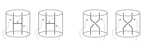
Figure 3. The arcs $\boldsymbol{a},\boldsymbol{a}^{\prime},\boldsymbol{b},\boldsymbol{b}^{\prime},c,c^{\prime}\subset\big{(}D\times[0,1]\big{)}\sqcup\big{(}D^{\prime}\times[0,1]\big{)}$.

From now on let $M$ be the disjoint union of $D\times[0,1]$ and $D^{\prime}\times[0,1]$, in symbols

$$M=\big{(}D\times[0,1]\big{)}\sqcup\big{(}D^{\prime}\times[0,1]\big{)},$$

where $D$ and $D^{\prime}$ respectively denote a copy of the $2$-disc $D^{2}$. Consider the two sets of properly embedded, framed (by the blackboard-framing) arcs $\boldsymbol{a},\boldsymbol{a}^{\prime},\boldsymbol{b},\boldsymbol{b}^{\prime}\subset M$ indicated in Figure 3. Understand these arcs as oriented upwards and consider the corresponding manifolds $\#_{\boldsymbol{a}}M$ and $\#_{\boldsymbol{b}}M$. Furthermore let $K,K^{\prime}\subset\#_{\boldsymbol{a}}M$ denote the framed knots indicated in Figure 4. The framings are measured with respect to $\Sigma^{\prime}\subset\#_{\boldsymbol{a}}M$, the genus-$1$ surface with two boundary components obtained by the $2$-fold connected sum of $D$ and $D^{\prime}$. Observe that $\#_{\boldsymbol{a}}M$ is naturally diffeomorphic to $\Sigma^{\prime}\times[0,1]$.

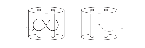
Figure 4. The knots $K$ and $K^{\prime}$ sitting in $\#_{\boldsymbol{a}}M$. Framings are measured with respect to $\Sigma^{\prime}\subset\#_{\boldsymbol{a}}M$.

Lemma 4.

Denote by $(\#_{\boldsymbol{a}}M)(K,K^{\prime})$ the result of surgery along $K_{0},K_{1}$ with respect to their framings (cf. Figure 4). Then we have

$$\#_{\boldsymbol{b}}M\cong(\#_{\boldsymbol{a}}M)(K,K^{\prime}).$$

Proof.

Let us give an explicit description of $M=\big{(}D\times[0,1]\big{)}\sqcup\big{(}D^{\prime}\times[0,1]\big{)}$ embedded in $\mathbb{R}^{3}$ with coordinates $(x,y,z)$: understand $D$ and $D^{\prime}$ as unit $2$-discs in the $xy$-plane centred at the points $(0,2)$ and $(0,-2)$. Identify $\boldsymbol{a},\boldsymbol{a}^{\prime}$ with $\{(\pm\frac{1}{2},2)\}\times[0,1]$ and $\{(\pm\frac{1}{2},-2)\}\times[0,1]$. Denote by $c,c^{\prime}$ the arcs given as $[-\frac{1}{2},\frac{1}{2}]\times\{\pm 2\}\times\{\frac{1}{2}\}$. Then $\#_{\boldsymbol{a}}M$ is given as the quotient

$$\Big{(}\big{(}D\times[0,1]\big{)}\setminus N_{\boldsymbol{a}}\Big{)}\cup\Big{(}\big{(}D^{\prime}\times[0,1]\big{)}\setminus N_{\boldsymbol{a}^{\prime}}\Big{)}/\sim_{\partial N_{\boldsymbol{a}}},$$

where we identify points $(x,y,z)\in\partial N_{\boldsymbol{a}}$ with their mirror image $(x,y,-z)\in\partial N_{\boldsymbol{a}^{\prime}}$. Note that the pair of arcs $c,c^{\prime}$ descends to the closed curve $K\subset\#_{\boldsymbol{a}}M$.

Denote by $H\subset M$ a neighbourhood of the graph $(a_{1}\cup a_{2})\cup c$. Choose $H^{\prime}$ to be the reflection of $H$ with respect to the $xz$-plane and note that $H^{\prime}$ provides a neighbourhood of the graph $(a^{\prime}_{1}\cup a^{\prime}_{2})\cup c^{\prime}$. Observe that the result $(\#_{\boldsymbol{a}}M)(K)$ of zero-surgery along $K$ is given by

$$\Big{(}\big{(}D\times[0,1]\big{)}\setminus H\Big{)}\cup\Big{(}\big{(}D^{\prime}\times[0,1]\big{)}\setminus H^{\prime}\Big{)}/\sim_{\partial H},$$

where we identify a point $(x,y,z)\in\partial H$ with its mirror $(x,-y,z)\in\partial H^{\prime}$.

Let us now perform the surgery along $K^{\prime}$. Isotope $K^{\prime}$ such that it lies on $\partial H$ sitting inside of $\#_{\boldsymbol{a}}M$. Note that the framing of $K^{\prime}$ and the framing induced by $\partial H$ agree. Let $\nu K^{\prime}=(-\varepsilon,\varepsilon)\times S^{1}$ denote a small open neighbourhood of $K^{\prime}$ in $\partial H$. Remove a neighbourhood $N_{K^{\prime}}\subset(\#_{\boldsymbol{a}}M)(K)$ of $K^{\prime}$ and observe that topologically the complement of $N_{K^{\prime}}$ is given by

(4) $$\Big{(}\big{(}D\times[0,1]\big{)}\setminus H\Big{)}\cup\Big{(}\big{(}D^{\prime}\times[0,1]\big{)}\setminus H^{\prime}\Big{)}/\sim_{\partial H\setminus\nu K^{\prime}},$$

where we just identify points $(x,y,z)\in\partial H\setminus\nu K^{\prime}$ with their mirror $(x,-y,z)\in\partial H^{\prime}$. We will glue back the surgery torus $S^{1}\times D^{2}$ in two steps. Take $[0,\pi]\times D^{2}\subset S^{1}\times D^{2}$ (where we identify $S^{1}\equiv\mathbb{R}/2\pi\mathbb{Z}$) and attach it along $[0,\pi]\times\partial D^{2}$ to the closure of the neighbourhood $\nu K^{\prime}\subset\partial H$, which we identify with $[-\varepsilon,\varepsilon]\times S^{1}$. Simultaneously attach $[\pi,2\pi]\times D^{2}$ along $[\pi,2\pi]\times\partial D^{2}$ to the mirror image of $\nu K^{\prime}$ on $\partial H^{\prime}$. We can actually picture this to be done inside of $H$ and $H^{\prime}$ respectively. Observe that the two pieces $\big{(}[0,\pi]\times D^{2}\big{)},\big{(}[\pi,2\pi]\times D^{2}\big{)}$, attached to the complement described in description (4) above, really descend to a solid torus. Moreover observe that we can understand the boundary of $N_{\boldsymbol{b}}$ as decomposes as $(\partial H\setminus\nu K^{\prime})\cup(\{0,\pi\}\times D^{2})$. Hence gluing back the surgery torus to the space given in (4) gives

$$\Big{(}\big{(}D\times[0,1]\big{)}\setminus N_{\boldsymbol{b}}\Big{)}\cup\Big{(}\big{(}D^{\prime}\times[0,1]\big{)}\setminus N_{\boldsymbol{b}^{\prime}}\Big{)}/\sim_{\partial N_{\boldsymbol{b}}},$$

which describes $\#_{\boldsymbol{b}}M$. This completes the proof. ∎

Figure 5. Two identifications of $\Sigma^{\prime}$ with the curves $\alpha,\beta,\gamma,\delta$ used in Lemma 5.

Recall that $\Sigma^{\prime}$ denotes the genus-$1$ surface with two boundary components understood as obtained by the $2$-fold connected sum of $D$ and $D^{\prime}$. Recall further $\#_{\boldsymbol{a}}M$ is naturally isomorphic to $\Sigma^{\prime}\times[0,1]$. We would now like to express the surgery along $K,K^{\prime}\subset\#_{\boldsymbol{a}}M$ in the above description of $\#_{\boldsymbol{b}}M$ as a sequence of $\pm 1$-surgeries along certain curves on $\Sigma^{\prime}$, where the framing is measured with respect to $\Sigma^{\prime}$.

Lemma 5.

Let $\alpha,\beta,\gamma,\delta\subset\Sigma^{\prime}$ denote the curves described in Figure 5. Then setting $\psi=(\tau_{\alpha}\tau_{\beta}\tau_{\gamma})^{2}(\tau_{\delta})^{-1}$ we have

$$(\#_{\boldsymbol{a}}M)(K,K^{\prime})=\Big{(}\big{(}\Sigma^{\prime}\times[0,1]\big{)}\cup\big{(}\Sigma^{\prime}\times[2,3]\big{)}\Big{)}/\sim_{\psi},$$

where we identify $(p,1)$ with $(\psi(p),2)$ for each $p\in\Sigma^{\prime}$.

Proof.

Recall that in Lemma 4 we identified $(\#_{\boldsymbol{a}}M)(K,K^{\prime})$ with $\#_{\boldsymbol{b}}M$. Observe that the latter space admits the structure of a $\Sigma^{\prime}$-fibration which is induced by the projection on the unit interval $[0,1]$. The map $\psi$ is actually a factorisation of the monodromy of this fibration into Dehn twists. A little caution is needed: unfortunately we are actually computing the inverse of $\psi$, since in our computations we push arcs from the top to the bottom, not the other way round.

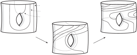
Figure 6. A cut system for $\Sigma^{\prime}$ and its image under $P\circ\psi^{-1}$.

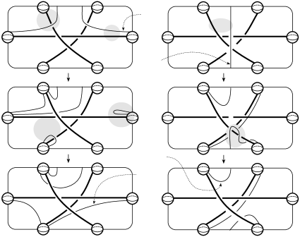
Figure 12. The images of $B$ and $C$ under $\psi^{-1}$. The shaded areas indicate that an isotopy or a handle slide is performed.

Let $A,B,C\subset\Sigma^{\prime}$ denote the cut system given in the left part of Figure 6. The images of this cut system under $\psi^{-1}$ are given in the middle part of Figure 6. The images were computed as follows: recall that $\#_{\boldsymbol{a}}M$ did correspond to $\Sigma^{\prime}\times[0,1]$ which we understand as obtained by thicken up the shaded area in Figure 5 (or Figure 7 respectively). A description of the knots $K,K^{\prime}$ with respect to this perspective is given in Figure 7. Understand the result of surgery $(\#_{\boldsymbol{a}}M)(K,K^{\prime})$ on $K,K^{\prime}$ as embedded in the Kirby diagram given in Figure 7. We can now recover the cut system, chosen above, in the Kirby diagram and manipulate it using Kirby calculus. The actual computations are given in Figures 11, 12 and LABEL:fig:image_C on p. 11ff at the end of the paper.

We could now just compare these images with the ones under the inverse of $(\tau_{\alpha}\tau_{\beta}\tau_{\gamma})^{2}(\tau_{\delta})^{-1}$ and conclude that both agree up to isotopy, showing that $\psi=(\tau_{\alpha}\tau_{\beta}\tau_{\gamma})^{2}(\tau_{\delta})^{-1}$.

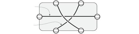
Figure 7. A Kirby diagram showing $K,K^{\prime}$ and $\Sigma^{\prime}$.

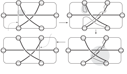
Figure 13. Computation of the image of $\alpha$ under $\psi^{-1}$. The shaded areas indicate that an isotopy or a handle slide is performed.

However the usual way to compute the factorisation of a monodromy map of a compact surface is by by reducing it to the case of a self-diffeomorphism of a disc with punctures, cf. [MR1414898]. Referring to Figure 13 (on p. 13) the image of $\alpha$ under $\psi^{-1}$ is given as $\beta$. Set

$$P=\tau_{\gamma}\thinspace\tau_{\beta}\thinspace\tau_{\alpha}\thinspace\tau_{\gamma}$$

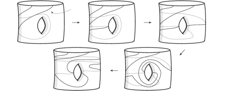
Figure 15. Computation of the image of $\psi^{-1}(B)$ under $P=\tau_{\gamma}\thinspace\tau_{\beta}\thinspace\tau_{\alpha}\thinspace\tau_{\gamma}$.

and note that $P$ maps $\beta$ to $\alpha$. Therefore $P\circ\psi^{-1}$ fixes the curve $\alpha$ and hence can now be interpreted as a self-diffeomorphism of the $3$-fold punctured disc $D_{3}$ obtained by cutting $\Sigma^{\prime}$ along $\alpha$. Note that $A,B\subset\Sigma^{\prime}$ descends to a cut system of $D_{3}=\Sigma^{\prime}\setminus\alpha$. Therefore all the data of $P\circ\psi^{-1}$ is encoded in the images of $A,B\subset\Sigma^{\prime}$. The images of $A,B\subset\Sigma^{\prime}$ under $P\circ\psi^{-1}$ are given in the right part of Figure 6 (cf. Figure 14 and Figure 15 on p. 14 and 15 for the actual computations). We conclude that we have

$$P\circ\psi^{-1}=\tau_{\alpha}^{-1}\thinspace\tau_{\beta}^{-1}\thinspace\tau_{\delta}.$$

Therefore $\psi^{-1}$ is given by $(\tau_{\alpha}^{-1}\thinspace\tau_{\beta}^{-1}\thinspace\tau_{\delta})\circ P^{-1}$, which, computing the inverse, is exactly what we intended to show. ∎

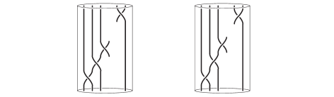
Figure 8. Description of the standard braids.

With this in hand we are able to compute the monodromy $\phi$ for the case that $K_{0}$ and $K_{1}$ are chosen among the standard braids $S^{+},S^{-}$ given in Figure 8.

Proposition 6.

Let $\alpha_{1},\ldots,\alpha_{n},\gamma_{1},\ldots,\gamma_{n-1},\delta^{(\prime)}_{1,2},\ldots,\delta^{(\prime)}_{n-1,n}\subset\Sigma$ denote the curves indicated in Figure 9. Then we have

• $\phi=\prod_{i=1}^{n-1}\tau_{\gamma_{i}}\thinspace\tau_{\alpha_{i}}\thinspace\tau_{\alpha_{i+1}}\thinspace\tau_{\gamma_{i}}$, for the pair of knots $(K_{0},K_{1})=(S^{+},S^{+})$,

• $\phi=\prod_{i=1}^{n-1}(\tau_{\gamma_{i}}\thinspace\tau_{\alpha_{i}}\thinspace\tau_{\alpha_{i+1}})^{2}\thinspace(\tau_{\delta_{i,i+1}})^{-1}$, for the pair of knots $(K_{0},K_{1})=(S^{-},S^{+})$ and

• $\phi=\prod_{i=1}^{n-1}\tau_{\alpha_{i}}\thinspace\tau_{\alpha_{i+1}}\thinspace(\tau_{\gamma_{i}}\thinspace\tau_{\alpha_{i}}\thinspace\tau_{\alpha_{i+1}})^{2}\thinspace(\tau_{\delta_{i,i+1}})^{-1}\thinspace(\tau_{\delta^{\prime}_{i,i+1}})^{-1}$, for the pair of knots $(K_{0},K_{1})=(S^{-},S^{-})$.

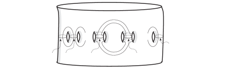
Figure 9. The curves used in Corollary 6 and Proposition 7.

Proof.

We start by proving the second part of the statement. Let $n\in\mathbb{N}$ be the braid index of $K_{0}$ and $K_{1}$ respectively. Consider two copies $L_{0},L_{1}$ of the trivial braid of $n$-strands describing an $n$-component unlink and perform a fibre connected sum for each pair of unknots. By applying Lemma 4 exactly $n-1$ times we can turn this $n$-fold fibre connected sum into the fibre connected sum along $S^{+}$ and $S^{-}$. Keeping track of the change of monodromy completes the proof of the second part.

Figure 10. Switching between positive and negative crossings.

In Lemma 4 we are considering the result of fibre summing a negative crossing (the arcs $a_{1},a_{2}$) with a positive one (the arcs $b_{1},b_{2}$). Perform a surgery as indicated in the left part of Figure 10 (or right part of Figure 10 respectively) and observe that we turned the negative (or positive respectively) crossing into a positive (or negative respectively) crossing. This actually is nothing but a certain Rolfsen twist. However by performing one of these surgeries we can always set up the situation for which Lemma 4 applies. Translating the surgery into the language of Dehn twists sets the way to compute the monodromy for the remaining cases and we are done. ∎

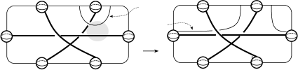
Figure 11. The shaded area indicates that a handle slide is performed.

3.2. Final computation of the monodromy

We almost have everything in place to compute the monodromy map $\phi$ of the fibre sum along multi-sections (see description (3) at the beginning of the section). The last ingredient is the following normal form for a braided knot $K$. Let $B$ be a braid representation of $K\subset S^{3}$ with braid index $n\in\mathbb{N}$ and let $S=S^{+}$ be the positive standard braid indicated in the right part of Figure 8. By an isotopy of $K$ we may assume that the permutation induced by $B$ is given by $(n\ 1\ \ldots\ n-1)$. Therefore $P=B\ast S^{-1}$ describes a pure braid for which we obviously have $B=P\ast S$. Here “$\ast$” denotes the composition of braids in the braid group.

According to [MR1414898] one can assign a pure braid to a diffeomorphism of the $n$-fold punctured disc, equal to the identity near the boundary, and vice versa. Let $\phi_{K}$ denote the map corresponding to the pure braid $P$ (which itself, by the consideration above, is induced by $K$ ). Note that the map $\phi_{K}$ encodes all information about $K$.

Let us return to the open book description $(\Sigma,\phi)$ of the fibre sum along $K_{0}$ and $K_{1}$ (cf. (3) above). Denote by $\phi_{K_{0}}$ and $\phi_{K_{1}}$ the maps associated to the knots $K_{0}$ and $K_{1}$ as described above. These maps trivially extend to $\Sigma$. Together with the first part of Proposition 6 we finally obtain the following description of $\phi$.

Theorem 7.

The monodromy $\phi$ of the open book described in (3) is given by

$$\phi=\Big{(}\prod_{i=1}^{n-1}\tau_{\gamma_{i}}\thinspace\tau_{\alpha_{i}}\thinspace\tau_{\alpha_{i+1}}\thinspace\tau_{\gamma_{i}}\Big{)}\circ\phi_{K_{0}}\circ\phi_{K_{1}},$$

where $\phi_{K_{0}}$, $\phi_{K_{1}}$ are as described above and $\alpha_{1},\ldots,\alpha_{n},\gamma_{1},\ldots,\gamma_{n-1}\subset\Sigma$ denote the curves indicated in Figure 9. ∎

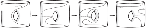
Figure 14. Computation of the image of $\psi^{-1}(A)$ under $P=\tau_{\gamma}\thinspace\tau_{\beta}\thinspace\tau_{\alpha}\thinspace\tau_{\gamma}$.

References

- \bibselectbib