Integrability as a consequence of discrete holomorphicity: the $\mathrm{Z}_{N}$ model

Abstract

It has recently been established that imposing the condition of discrete holomorphicity on a lattice parafermionic observable leads to the critical Boltzmann weights in a number of lattice models. Remarkably, the solutions of these linear equations also solve the Yang-Baxter equations. We extend this analysis for the $\mathrm{Z}_{N}$ model by explicitly considering the condition of discrete holomorphicity on two and three adjacent rhombi. For two rhombi this leads to a quadratic equation in the Boltzmann weights and for three rhombi a cubic equation. The two-rhombus equation implies the inversion relations. The star-triangle relation follows from the three-rhombus equation. We also show that these weights are self-dual as a consequence of discrete holomorphicity.

1 Introduction

In some remarkable developments, a surprising connection has been uncovered between the notions of discrete holomorphicity and Yang-Baxter integrability [1, 2, 3, 4, 5]. On the one hand, a parafermionic observable on the lattice is discretely holomorphic, i.e., the observable satisfies a version of the discrete Cauchy-Riemann equations. This requirement leads to a set of linear equations which can be solved to yield the Boltzmann weights of the model at criticality. The surprise is that, on the other hand, these are the same Boltzmann weights that follow by solving the star-triangle or Yang-Baxter equations. This connection has been observed by Rajabpour and Cardy [1] for the $\mathrm{Z}_{N}$ model and by Ikhlef and Cardy [2] for the Potts model, the dilute $O(n)$ loop model and the dilute $C_{2}^{(1)}$ loop model. This list also includes the Ashkin-Teller model [4, 5].

As yet there is no satisfactory explanation for this unexpected connection between discrete holomorphicity and Yang-Baxter integrability. Our aim in this paper is to explicitly establish that the star-triangle equation, and thus Yang-Baxter integrability, is a consequence of discrete holomorphicity. We will do this in the context of general rhombi on a Baxter lattice and the $\mathrm{Z}_{N}$ model. Our approach is thus algebraic.

The utility and power of the Yang-Baxter equation is well known. The importance and full power of discrete holomorphicity is becoming increasingly recognised. Setting up a discretely holomorphic observable has been a very useful step for the passage from discrete lattice models to the continuous functions of conformal field theory [6, 7]. Among other examples, discrete holomorphicity is a key ingredient in Duminil-Copin and Smirnov’s [8] remarkable and long sought after rigorous proof of the connective constant for self-avoiding walks on the honeycomb lattice. The exact value had been obtained 30 years ago by Nienhuis [9] in the $n=0$ limit of the $O(n)$ loop model on the honeycomb lattice. Nienhuis used various mappings between the vertex weights of different lattice models. The key point is that for $n=0$ all contributions from closed loops vanish, leaving only self-avoiding walks. The crucial first step in the arguments used by Duminil-Copin and Smirnov is the introduction of a parafermionic observable on the lattice which is discretely holomorphic. The second step involved the use of counting arguments in a domain of the hexagonal lattice. This step built on previous rigorous mathematical results obtained for decomposition of excursions across finite domains. A more formal proof has been given by Klazar [10]. The fact that such exact and rigorous results exist is no doubt related to the underlying integrability of the $O(n)$ loop model on the honeycomb lattice [11].

The arguments used by Duminil-Copin and Smirnov [8] were extended to the $O(n)$ loop model on the honeycomb lattice with a boundary by Beaton, Bousquet-Melou, de Gier, Duminil-Copin and Guttmann [12] to give a mathematically rigorous proof for the critical surface adsorption temperature of self-avoiding walks on the honeycomb lattice. This polymer adsorption transition corresponds to the $n=0$ limit of the $O(n)$ model at the special surface transition. The exact value for the adsorption transition had been obtained earlier by Batchelor and Yung [13] from the boundary Boltzmann weights obtained by solving the boundary version of the Yang-Baxter equation. Discrete holomorphicity at a boundary has been considered by Ikhlef [14] who was able to recover the boundary weights of the $O(n)$ loop model on the square lattice and to obtain a new set of boundary weights for the $\mathrm{Z}_{N}$ model.

2 From discrete holomorphicity to the star-triangle equation

For a $\mathrm{Z}_{N}$ symmetric $N$-state spin model on a graph, the weight $w(s_{a},s_{b})$ of the interaction on an edge ${\langle{a},{b}\rangle}$ is unchanged by the global transformations $s_{r}\mapsto\omega s_{r}$ and $s_{r}\mapsto s_{r}^{*}$ of the spins. Here the spins take values from the $N$th roots of unity, $s_{r}=\omega^{q_{r}}$, with $q_{r}\in\{0,1,\ldots,N-1\}$ and $\omega=\exp\left({{2\pi\rmi/N}}\right)$. For a review of these models and other important models contained therein, such as the Ising and Potts models, see, e.g., [15].

Since the weight depends only on the difference of the $q_{r}$ variables, we write it as $W(q_{a}-q_{b})$, or, by a slight abuse of notation, simply $W(a-b)$. The Kramers-Wannier duality of the model [16] lets one define disorder variables $\mu_{\tilde{{r}}}$ dual to the spins on the dual graph. The effect of inserting a disorder variable at the dual site $\tilde{r}$ is to introduce a string connecting the site to a site at infinity or at the boundary. Whenever the string intersects an edge of the original lattice, it modifies the weight on that edge by, for definiteness, lowering the spin $q_{r}$ to its right by one.

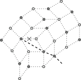
Figure 1: A rhombic embedding of the covering lattice of a heterogeneous model showing a string attached to a disorder variable. The empty circles denote the spin variables, while the full circles denote the disorder variables. The location of the parafermion is marked with an $\times$.

We consider a rhombic embedding of the covering lattice, the union of the original lattice and its dual, onto the complex plane (figure 1). Each elementary rhombus of this lattice contains an edge from the original lattice and an edge from the dual lattice. The parafermion introduced by Rajabpour and Cardy [1]

$$\psi_{{\langle{r},{\tilde{r}}\rangle}}=\exp\left({-\rmi\,\sigma\,\theta_{{\langle{r},{\tilde{r}}\rangle}}}\right)\cdot s_{r}\cdot\mu_{\tilde{{r}}}$$

lives on the midpoint of the edges. Here, the angle $\theta_{{\langle{r},{\tilde{r}}\rangle}}$ is the angle between the edge traversed from the spin to the disorder variable and an arbitrary but fixed axis. The real parameter $\sigma$ can be identified as the conformal spin of the observable. When the string enters a particular rhombus of opening angle $\alpha$ through the disorder variable $\mu_{\tilde{{X}}}$ (figure 2), imposing the condition of discrete holomorphicity

$$\sum_{\lozenge}\psi_{{\langle{r},{\tilde{r}}\rangle}}\,\Delta z_{{\langle{r},{\tilde{r}}\rangle}}=0$$ (1)

on the contour sum of the parafermion around the rhombus in the counterclockwise direction we get,

$$-\rme^{\rmi\,\sigma\,\pi}\,s_{g}\,\mu_{\tilde{{Y}}}-\rme^{\rmi\,(1-\sigma)\,\alpha}\,s_{a}\,\mu_{\tilde{{Y}}}+s_{a}\,\mu_{\tilde{{X}}}+\rme^{\rmi\,\sigma\,\pi}\,\rme^{\rmi\,(1-\sigma)\,\alpha}\,s_{g}\,\mu_{\tilde{{X}}}=0$$

where the variables $s_{a}$, $\mu_{\tilde{{X}}}$, $s_{g}$, $\mu_{\tilde{{Y}}}$ are at the corners of the contour, in that order, and $\Delta z$ is the difference between the complex coordinates of the two endpoints of the side of the rhombus on which the $\psi_{{\langle{r},{\tilde{r}}\rangle}}$ variable lives, traversed in the direction of traversal of the contour.

As was explained in [1, 14], we have taken the special case $m=1$ of the more general definition of the parafermion

$$\psi^{(m)}_{{\langle{r},{\tilde{r}}\rangle}}=\exp\left({-\rmi\,\sigma_{m}\,\theta_{{\langle{r},{\tilde{r}}\rangle}}}\right)\cdot s^{m}_{r}\cdot\mu^{(m)}_{\tilde{r}}$$

where the string attached to the disorder variable $\mu^{(m)}_{\tilde{r}}$ modifies the weight of an edge it crosses by lowering the spin to its right by $m$, and $m\in\{1,\ldots,N-1\}$. These observables, which are also discretely holomorphic at integrable critical points, are related to the one we consider by the global transformation $s_{r}\mapsto{s^{m}_{r}}$, and thus, it is enough to consider the $m=1$ case only without loss of generality.

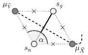
Figure 2: An elementary rhombus with opening angle $\alpha$. The string enters the rhombus via the disorder variable $\mu_{\tilde{{X}}}$. The arbitrary axis is in the direction of the edge ${\langle{a},{X}\rangle}$.

With the introduction of $\phi(\alpha)=\rme^{\rmi\,(1-\sigma)\,\alpha}$, the condition takes the form

$$\phi(-\pi)\,s_{g}\,\mu_{\tilde{{Y}}}-\phi(\alpha)\,s_{a}\,\mu_{\tilde{{Y}}}+s_{a}\,\mu_{\tilde{{X}}}-\phi(\alpha-\pi)\,s_{g}\,\mu_{\tilde{{X}}}=0$$ (2)

Since, by our characterization of the disorder variables,

$$\frac{\mu_{\tilde{{Y}}}}{\mu_{\tilde{{X}}}}=\frac{W_{\alpha}(a-(g-1))}{W_{\alpha}(a-g)}=\frac{W_{\alpha}(n_{a}+1)}{W_{\alpha}(n_{a})}$$

we have

$$\left({\phi(-\pi)-\phi(\alpha)\,\omega^{n_{a}}}\right)W_{\alpha}(n_{a}+1)+\left({\omega^{n_{a}}-\phi(\alpha-\pi)}\right)W_{\alpha}(n_{a})=0$$ (3)

which is a linear recurrence relation in the weights in terms of the bond varible $n_{a}$.

This relation specifies the weights up to a physically irrelevant constant. The $\mathrm{Z}_{N}$ symmetries, however, put constraints on the value of the unknown $\sigma$ (see, e.g., [14]). Since the weights are symmetric and periodic, we must have $W_{\alpha}(n_{a})=W_{\alpha}(N-n_{a})$ for every $n_{a}$, from which the recurrence relation gives

$$\left({1-\phi(2\alpha)}\right)\left({\omega^{-1}-\phi(-2\pi)}\right)=0$$

Taking

$$\phi(2\pi)=\omega$$ (4)

makes the parafermion holomorphic for every opening angle $\alpha$. Therefore,

$$\sigma=1-\frac{1}{N}+\ell$$ (5)

for any integer $\ell$. The case $\ell=0$ gives the Fateev-Zamolodchikov solutions [17]. Since the subsequent calculations make use of relation (4) and not the actual value of $\sigma$, the proof presented here is more general than merely proving that the Fateev-Zamolodchikov weights give us an integrable model. The angle $\alpha$ is proportional to (in fact, in [17], equal to) the spectral parameter and plays an analogous rôle.

It should be noted that the weights are real because the ratio of the weights given by the recurrence relation (3) is real.

2.1 Self-duality

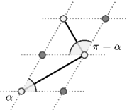
Figure 3: Rhombic embedding of an anisotropic square lattice. The edge with an opening angle $\alpha$ is horizontal, while that with an opening angle $\pi-\alpha$ is vertical in the original lattice.

We now show that the weights are self-dual. For this, we temporarily consider the embedding of an anisotropic square lattice (figure 3). On the one hand, if the horizontal interaction edges are mapped onto rhombi of opening angle $\alpha$, the vertical edges are then mapped onto rhombi with opening angle $\pi-\alpha$. We thus have $\overline{W}_{\alpha}(n_{a})=W_{\pi-\alpha}(n_{a})$. On the other hand, taking the discrete Fourier transform of the recurrence relation (3) we have

$$\left({\phi(-\pi)-\phi(-\pi-\alpha)\,\omega^{k_{a}+1}}\right)\widetilde{W}_{\alpha}(k_{a}+1)+\left({\omega^{k_{a}}-\phi(-\alpha)}\right)\widetilde{W}_{\alpha}(k_{a})=0$$

Using (4) to replace the extra $\omega$ in the first term, we see that the dual weights satisfy the same equation with $\alpha$ replaced by $\pi-\alpha$. Since our unitary Fourier transform preserves the norm

$$\sum_{n_{a}\in\mathrm{Z}_{N}}[W_{\alpha}(n_{a})]^{2}=1$$ (6)

this proves

$$\overline{W}_{\alpha}(n_{a})=W_{\pi-\alpha}(n_{a})=\widetilde{W}_{\alpha}(n_{a})$$ (7)

and captures the crossing symmetry of the problem.

2.2 Inversion relations

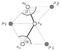
Figure 4: Two adjacent rhombi.

Now we consider another rhombus with angle $\beta$ which sits on top of the rhombus considered so far (figure 4). The new rhombus comes with spin $s_{b}$ and disorder variable $\mu_{\tilde{{Z}}}$ and shares the edge ${\langle{g},{\tilde{Y}}\rangle}$ with the previous one. We multiply its holomorphicity equation analogous to (2) by $\phi(-\beta)$ to orient it correctly and then add the two equations to get

$$-\phi(\alpha)\,s_{a}\,\mu_{\tilde{{Y}}}+s_{a}\,\mu_{\tilde{{X}}}-\phi(\alpha-\pi)\,s_{g}\,\mu_{\tilde{{X}}}$$

$$\quad\quad+\,\phi(-\pi-\beta)\,s_{g}\,\mu_{\tilde{{Z}}}-s_{b}\,\mu_{\tilde{{Z}}}+\phi(-\beta)\,s_{b}\,\mu_{\tilde{{Y}}}=0$$ (8)

The contributions from the common edge cancel as it is traversed in opposite directions for the two sums. Using

$$\frac{\mu_{\tilde{{Z}}}}{\mu_{\tilde{{Y}}}}=\frac{W_{\beta}(b-(g-1))}{W_{\beta}(b-g)}=\frac{W_{\beta}(n_{b}+1)}{W_{\beta}(n_{b})}$$

the equation (2.2) gives a quadratic relation

$$\left({\omega^{a}-\phi(\alpha-\pi)\,\omega^{g}}\right)W_{\alpha}(n_{a})\,W_{\beta}(n_{b})$$

$$\quad\quad+\,\left({\phi(-\beta)\,\omega^{b}-\phi(\alpha)\,\omega^{a}}\right)W_{\alpha}(n_{a}+1)\,W_{\beta}(n_{b})$$

$$\quad\quad+\,\left({\phi(-\pi-\beta)\,\omega^{g}-\omega^{b}}\right)W_{\alpha}(n_{a}+1)\,W_{\beta}(n_{b}+1)=0$$ (9)

in the weights.

This relation contains the inversion relations (see, e.g., [18]) for the model. Put $a=b$, so that $n_{a}=n_{b}=n$, and $\beta=-\alpha$, then the equation reduces to

$$W_{\alpha}(n)\,W_{-\alpha}(n)=W_{\alpha}(n+1)\,W_{-\alpha}(n+1)$$

thus, the product is independent of $n$,

$$W_{\alpha}(n)\,W_{-\alpha}(n)=g(\alpha)\,g(-\alpha)$$ (10)

The other relevant inversion relation

$$\sum_{g\in\mathrm{Z}_{N}}W_{\pi+\theta}(a-g)\,W_{\pi-\theta}(b-g)=\rho(\theta)\,\delta_{a,b}$$ (11)

follows from this relation and self-duality by expanding the left hand side in Fourier coefficients and gives

$$\rho(\theta)=N\,g(\theta)\,g(-\theta)$$

for our normalization.

2.3 Star-triangle relation

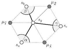
Figure 5: Three adjacent rhombi making the star.

We proceed to add the third rhombus with angle $\gamma=2\pi-(\alpha+\beta)$ to make the star (figure 5). Two of the edges, ${\langle{g},{\tilde{Z}}\rangle}$ and ${\langle{g},{\tilde{X}}\rangle}$, are shared and a new spin variable $s_{c}$ is introduced. Multiplying the holomorphicity equation analogous to (2) for this rhombus by $\phi(2\pi-\alpha)$ to orient it correctly, we add it to the contour sum (2.2) to yield

$$\phi(\alpha-3\pi)\,s_{g}\,\bar{\mu}_{\tilde{X}}-\phi(\alpha-\pi)\,s_{g}\,\mu_{\tilde{{X}}}$$

$$\quad\quad+\,s_{a}\,\mu_{\tilde{{X}}}-\phi(\alpha)\,s_{a}\,\mu_{\tilde{{Y}}}$$

$$\quad\quad+\,\phi(-\beta)\,s_{b}\,\mu_{\tilde{{Y}}}-s_{b}\,\mu_{\tilde{{Z}}}$$

$$\quad\quad+\,\phi(\alpha-2\pi)\,s_{c}\,\mu_{\tilde{{Z}}}-\phi(-\beta)\,s_{c}\,\bar{\mu}_{\tilde{X}}=0$$ (12)

Some features of this equation warrant attention. The disorder variable $\mu_{\tilde{{X}}}$ is not the same as $\bar{\mu}_{\tilde{X}}$, as might be naïvely expected. A possible interpretation of this is that the string has gone around the spin $s_{g}$ once, and thus the parafermion has acquired a phase factor $\phi(2\pi)$, corresponding to the lowering of the value of $g$, that is, $q_{g}$, by one in the configuration. Hence, the contributions from the edge ${\langle{g},{\tilde{X}}\rangle}$ do not cancel.

Making use of

$$\frac{\bar{\mu}_{\tilde{X}}}{\mu_{\tilde{{Y}}}}=\frac{W_{\gamma}(c-(g-1))}{W_{\gamma}(c-g)}=\frac{W_{\gamma}(n_{c}+1)}{W_{\gamma}(n_{c})}$$

we have a cubic equation in weights which we omit for clarity. However, summing over $g$, we arrive at

$$\left({\omega^{a}-\phi(-\beta)\,\omega^{c}}\right)\,\mathfrak{L}_{\alpha,\beta}(a,b,c)$$

$$\quad\quad+\,\left({\phi(-\beta)\,\omega^{b}-\phi(\alpha)\,\omega^{a}}\right)\,\mathfrak{L}_{\alpha,\beta}(a+1,b,c)$$

$$\quad\quad+\,\left({\phi(\alpha-2\pi)\,\omega^{c}-\omega^{b}}\right)\,\mathfrak{L}_{\alpha,\beta}(a+1,b+1,c)=0$$ (13)

Here

$$\mathfrak{L}_{\alpha,\beta}(a,b,c)=\sum_{g\in\mathrm{Z}_{N}}W_{\alpha}(a-g)\,W_{\beta}(b-g)\,W_{\gamma}(c-g)$$ (14)

is the left hand side of the star-triangle relation. The terms involving $s_{g}$ cancel because of the constraint (4) on $\sigma$, and therefore, the expectation value of the parafermion is still independent of the path, as is that for the disorder variable $\mu_{\tilde{{X}}}$, and consequently the contour sum around the star still vanishes.

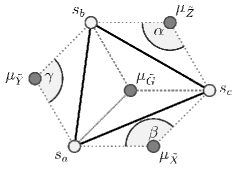
Figure 6: Three adjacent rhombi making the triangle.

Remarkably, considering the contour sum around the triangle (figure 6), we get

$$\left({\omega^{a}-\phi(-\beta)\,\omega^{c}}\right)\,\mathfrak{R}_{\alpha,\beta}(a,b,c)$$

$$\quad\quad+\,\left({\phi(-\beta)\,\omega^{b}-\phi(\alpha)\,\omega^{a}}\right)\,\mathfrak{R}_{\alpha,\beta}(a+1,b,c)$$

$$\quad\quad+\,\left({\phi(\alpha-2\pi)\,\omega^{c}-\omega^{b}}\right)\,\mathfrak{R}_{\alpha,\beta}(a+1,b+1,c)=0$$ (15)

where

$$\mathfrak{R}_{\alpha,\beta}(a,b,c)=W_{\pi-\gamma}(a-b)\;W_{\pi-\alpha}(b-c)\;W_{\pi-\beta}(c-a)$$ (16)

is proportional to the right hand side of the star-triangle relation. The two sides of the equation therefore obey the same recurrence relation.

To show that the star-triangle relation follows from these relations, we have to prove that the two solutions are linearly dependent. To this end, we consider a general solution of the recurrence relation $f_{\alpha,\beta}(a,b,c)$. Taking the complex conjugate of the relation and noting both $f_{\alpha,\beta}(a,b,c)$ and $\sigma$ are real, we multiply the resulting equation by $\phi(\alpha-\beta)\,\omega^{a+b}$. The result,

$$\left({\phi(\alpha-\beta)\,\omega^{b}-\phi(\alpha)\,\omega^{a+b-c}}\right)\,f_{\alpha,\beta}(a,b,c)$$

$$\quad\quad+\,\left({\phi(\alpha)\,\omega^{a}-\phi(-\beta)\,\omega^{b}}\right)\,f_{\alpha,\beta}(a+1,b,c)$$

$$\quad\quad+\,\left({\phi(2\pi-\beta)\,\omega^{a+b-c}-\phi(\alpha-\beta)\,\omega^{a}}\right)\,f_{\alpha,\beta}(a+1,b+1,c)=0$$ (17)

when added to the recurrence relation, cancels the middle term and gives the ratio

$$\frac{f_{\alpha,\beta}(a+1,b+1,c)}{f_{\alpha,\beta}(a,b,c)}=\frac{f_{\alpha,\beta}(a,b,c-1)}{f_{\alpha,\beta}(a,b,c)}$$ (18)

independent of the function $f_{\alpha,\beta}$. The shift in the arguments is justified by the $\mathrm{Z}_{N}$ symmetries. Since this ratio is the same for both $\mathfrak{R}_{\alpha,\beta}$, and $\mathfrak{L}_{\alpha,\beta}$,

$$\frac{\mathfrak{L}_{\alpha,\beta}(a,b,c)}{\mathfrak{R}_{\alpha,\beta}(a,b,c)}=\frac{\mathfrak{L}_{\alpha,\beta}(a,b,c-1)}{\mathfrak{R}_{\alpha,\beta}(a,b,c-1)}$$ (19)

The ratio of the two sides is thus independent of the spin $c$. Similar elimination of the other two terms in the recurrence relation shows that the ratio is independent of $a$ and $b$ as well, as is demanded by symmetry. We therefore have the star-triangle relation

$$\mathfrak{L}_{\alpha,\beta}(a,b,c)=R_{\alpha,\beta}\,\mathfrak{R}_{\alpha,\beta}(a,b,c)$$ (20)

where $R_{\alpha,\beta}$ depends on the spectral variables only.

As is well-known, the inversion relations (10)-(11) and the star-triangle relation (20) together are sufficient to establish the existence of commuting transfer matrices parametrized by, in our case, the angle of the embedded rhombi, or in other words, Yang-Baxter integrability. By the embedding onto the complex plane, the schematic diagram of the Yang-Baxter equations acquires a geometric meaning of rearrangements of the elementary rhombi. Our analysis shows that the contour sum around a domain picks up only factors independent of the configuration under such rearrangements.

2.4 Homogeneous lattices

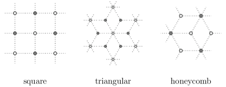
Figure 7: Rhombic embedding of the three homogeneous lattices.

It is interesting to note that the construction presented above is local in that it does not depend on many of the properties, e.g., the coordination number, of the underlying graph. To see the consequences of this lattice independence, we consider the three archetypical homogeneous lattices, the square, the triangular and the honeycomb (figure 7). The embedding of these lattices onto the complex plane tiles the plane with $\alpha$ being $\pi/2$, $\pi/3$ and $2\pi/3$ respectively. Evaluating the recurrence relation (3) at these points gives an instant derivation of the known critical weights. For example, for the Ising model, we have for $W(1)/W(0)$, the known values $\sqrt{2}-1$, $1/\sqrt{3}$, and $2-\sqrt{3}$ for the three lattices respectively [20].

3 Concluding remarks

In this paper, we considered the implication of the condition of discrete holomorphicity on two and three adjacent rhombi in the context of the lattice $\mathrm{Z}_{N}$ model. For two rhombi this led to the quadratic equation (2.2) in the Boltzmann weights. This equation was shown to imply the known inversion relations (10) and (11) for this model. Note that Cardy [21] has effectively established the inversion relations in the $u-v\to 0$ limit of the Yang-Baxter equation. For three rhombi we obtained the cubic equation (2.3) in the Boltzmann weights. In establishing this equation the lattice parafermion picks up a crucial phase factor, with the expectation value of the parafermion still independent of the path. The importance of such a phase factor has been highlighted in the topological context of the loop models by Fendley [22]. Here we have shown that the star-triangle relation (20) follows from the three-rhombus equation (2.3). In the discrete holomorphic approach the two-rhombus equation (2.2) and the three-rhombus equation (2.3) can thus be considered as analogues of the two- and three-body conditions for integrability. However, the simplicity of the discrete holomorphic approach is that ultimately these conditions are equivalent to the one-rhombus equation (2). Indeed, one can push this argument further by building up a transfer matrix from the rhombi and showing that commuting transfer matrices can be established as a consequence of discrete holomorphicity, bypassing the use of the Yang-Baxter equation. Our results lend further impetus for using discrete holomorphicity as a tool for investigating lattice models at critical points.

References

References

- [1] Rajabpour M A and Cardy J 2007 Discretely holomorphic parafermions in lattice models J. Phys. A 40 14703
- [2] Ikhlef Y and Cardy J 2009 Discretely holomorphic parafermions and integrable loop models J. Phys. A 42 102001
- [3] Cardy J 2009 Discrete holomorphicity at two-dimensional critical points J. Stat. Phys. 137 814
- [4] Lottini S and Rajabpour M A 2010 Ashkin-Teller model on the iso-radial graphs J. Stat. Mech. P06027
- [5] Ikhlef Y and Rajabpour M A 2011 Discrete holomorphic parafermions in the Ashkin-Teller model and SLE J. Phys. A 44 14703
- [6] Smirnov S 2010 Discrete complex analysis and probability In Proceedings of the International Congress of Mathematicians pp 595-621
- [7] Duminil-Copin H and Smirnov S 2011 Conformal invariance of lattice models arXiv:1109.1549v4
- [8] Duminil-Copin H and Smirnov S 2012 The connective constant of the honeycomb lattice equals Ann. of Math. 175 1653
- [9] Nienhuis B 1982 Exact critical point and critical exponents of models in two dimensions Phys. Rev. Lett.49 1062
- [10] Klazar M 2011 On the theorem of Duminil-Copin and Smirnov about the number of self-avoiding walks in the hexagonal lattice arXiv:1102.5733
- [11] Baxter R J 1986 colourings of the triangular lattice J. Phys. A 19 2821
- [12] Beaton N R, Bousquet-Melou M, de Gier J, Duminil-Copin H and Guttmann A J 2011 The critical fugacity for surface adsorption of self-avoiding walks on the honeycomb lattice is arXiv:1109.0358v3
- [13] Batchelor M T and Yung C M 1995 Exact results for the adsorption of a flexible self-avoiding polymer chain in two dimensions Phys. Rev. Lett.74 2026
- [14] Ikhlef Y 2012 Discretely holomorphic parafermions and integrable boundary conditions J. Phys. A 45 265001
- [15] Wu F Y 1982 The Potts model Rev. Mod. Phys. 54 235
- [16] Wu F Y and Wang Y K 1976 Duality transformation in a many-component spin model J. Math. Phys. 17 439
- [17] Fateev V A and Zamolodchikov A B 1982 Self-dual solutions of the star-triangle relations in -models Phys. Lett. A 92 37
- [18] Zhou Y K 1997 Fateev-Zamolodchikov and Kashiwara-Miwa models: boundary star-triangle relations and surface critical properties Nucl. Phys. B 487 779
- [19] Au-Yang H and Perk J H H 1989 Onsager’s star-triangle equation: master key to integrability, Proc. Taniguchi Symposium, Kyoto, October 1988, in: Advanced Studies in Pure Mathematics 19 (Kinokuniya-Academic, Tokyo) pp 57-94
- [20] Baxter R J 1982 Exactly solved models in statistical mechanics (Academic Press, London)
- [21] Cardy J 2012 Holomorphic parafermions on the lattice and in conformal field theory, talk given at the meeting Conformal Invariance, Discrete Holomorphicity and Integrability, Helsinki, June 10-16
- [22] Fendley P 2012 Discrete holomorphicity from topology, talk given at the meeting Conformal Invariance, Discrete Holomorphicity and Integrability, Helsinki, June 10-16