Time-evolution and dynamical phase transitions at a critical time in a system of one dimensional bosons after a quantum quench

Abstract

A renormalization group approach is used to show that a one dimensional system of bosons subject to a lattice quench exhibits a finite-time dynamical phase transition where an order parameter within a light-cone increases as a non-analytic function of time after a critical time. Such a transition is also found for a simultaneous lattice and interaction quench where the effective scaling dimension of the lattice becomes time-dependent, crucially affecting the time-evolution of the system. Explicit results are presented for the time-evolution of the boson interaction parameter and the order parameter for the dynamical transition as well as for more general quenches.

A fundamental and challenging topic of research is to understand nonequilibrium strongly correlated systems in general, and how phase transitions occur in such systems in particular. While the theory of equilibrium phase transitions is well developed, and relies heavily on the renormalization group, the development of an equally powerful approach to study nonequilibrium phase transitions is still in its infancy. Moreover, in any progress on this topic, it has always appeared that nonequilibrium phase transitions have one aspect in common with their equilibrium counterparts, both occur by adiabatically tuning some parameter of the system, in the absence or presence of an external drive, and strictly speaking occur only in the limit of infinite time (steady-state). Mitra et al. (2006); Mitra and Millis (2008); Diehl et al. (2010); Prosen and Ilievski (2011); Mitra and Giamarchi (2011, 2012); Shekhawat et al. (2011); Dalla Torre et al. (2012)

In contrast, here we study a completely different kind of a nonequilibrium phase transition, one that occurs as a function of time. Employing a time-dependent renormalization group (RG) approach we study quench dynamics of interacting one-dimensional (1D) bosons in a commensurate lattice. This system in equilibrium shows the Berezinskii-Kosterlitz-Thouless (BKT) transition separating a Mott insulating phase from a superfluid phase (Fig. 1). Giamarchi (2004) For the nonequilibrium situation we explicitly show the appearance of a dynamical phase transition where an order-parameter grows as a non-analytic function of time after a critical time. Such a behavior has no analog in equilibrium systems.

A dynamical transition in time was recently identified in the exactly solvable transverse field Ising model where the Loschmidt echo was found to show non-analytic behavior at a critical time, whereas the behavior of the order-parameter was analytic. Heyl et al. (shed) In contrast here we identify a situation where the order-parameter itself can show non-analyticities as a function of time. In addition we generalize the study of dynamical transitions to models that are not exactly solvable, and to low-dimensions where strong fluctuations negate a mean-field analysis. Sciolla and Biroli (2011)

We identify the dynamical transition by studying an order-parameter $\Delta(r,T_{m})$ which due to the quench depends both on position $r$ and a time $T_{m}$ after the quench. The phase transition is associated with a non-analytic behavior as a function of time $T_{m}$ on the value of this order-parameter spatially averaged within a light cone. Our results hold relevance not only to experiments in cold-atomic gases where system parameters can be tuned rapidly in time, Bloch et al. (2008) but also to conventional solid state materials where time-evolution of an order-parameter may be probed with high precision using ultra-fast pump-probe Fausti et al. (2011) and angle resolved photoemission spectroscopy. Smallwood et al. (2012)

We model the 1D Bose gas as a Luttinger liquid, Giamarchi (2004)

$$H_{i}=\frac{u_{0}}{2\pi}\int dx\left[K_{0}\left[\pi\Pi(x)\right]^{2}+\frac{1}{K_{0}}\left[\partial_{x}\phi(x)\right]^{2}\right]$$ (1)

where $-\partial_{x}\phi/\pi$ represents the density of the Bose gas, $\Pi$ is the variable canonically conjugate to $\phi$, $K_{0}$ is the dimensionless interaction parameter, and $u_{0}$ is the velocity of the sound modes. We assume that the bosons are initially in the ground state of $H_{i}$. The system is driven out of equilibrium via an interaction quench at $t$=$0$ from $K_{0}\rightarrow K$, with a commensurate lattice $V_{sg}$ also switched on suddenly, at the same time as the quench. This triggers non-trivial time-evolution from $t>0$ due to a Hamiltonian $H_{f}=H_{f0}+V_{sg}$, where $H_{f0}=H_{i}(K_{0}\rightarrow K)$ and $V_{sg}=-\frac{gu}{\alpha^{2}}\int dx\cos(\gamma\phi)$, with $g>0$, and $\Lambda=\frac{u}{\alpha}$ a short-distance cut-off. We assume that the quench preserves Galilean invariance so that $uK$=$u_{0}K_{0}$, however this is not critical for either the approach or the result. While $\gamma$=$2$ for bosons, we keep it general so that the results may be generalized to other 1D systems.

Figure 1: The equilibrium BKT phase diagram. Arrows connect the Hamiltonians before ($H_{i}$ ) and after ($H_{f}$) the quench. A dynamical phase transition is found for case (d).

In the absence of the lattice, the system is exactly diagonalizable in terms of the density modes, $H_{i}$=$\sum_{p\neq 0}u_{0}|p|\eta_{p}^{\dagger}\eta_{p}$ and $H_{f0}$= $\sum_{p\neq 0}u|p|\beta_{p}^{\dagger}\beta_{p}$ where $\beta,\eta$ are related by a canonical transformation. This fact has been used to study the dynamics of a Luttinger liquid exactly, and has revealed interesting physics arising from a lack of thermalization in the system. Cazalilla (2006); Iucci and Cazalilla (2009); Perfetto and Stefanucci (2011); Dóra et al. (2011) To study the system in the presence of the lattice employing RG, we write the Keldysh action representing the time-evolution from the initial pure state $|\phi_{i}\rangle$ (hence an initial density matrix $\rho=|\phi_{i}\rangle\langle\phi_{i}|$) corresponding to the ground state of $H_{i}$, $Z_{K}=Tr\left[\rho(t)\right]=Tr\left[e^{-iH_{f}t}|\phi_{i}\rangle\langle\phi_{i}|e^{iH_{f}t}\right]$ =$\int{\cal D}\left[\phi_{cl},\phi_{q}\right]e^{i\left(S_{0}+S_{sg}\right)}$. $S_{0}$ is the quadratic part which describes the nonequilibrium Luttinger liquid, which at a time $t$ after the quench is, not

$$S_{0}=\int_{-\infty}^{\infty}dx_{1}\int_{-\infty}^{\infty}dx_{2}\int_{0}^{t}dt_{1}\int_{0}^{t}dt_{2}\begin{pmatrix}\phi_{cl}(1)&\phi_{q}(1)\end{pmatrix}$$

$$\begin{pmatrix}0&&G_{A}^{-1}(1,2)\\ G_{R}^{-1}(1,2)&&-\left[G_{R}^{-1}G_{K}G^{-1}_{A}\right](1,2)\end{pmatrix}\begin{pmatrix}\phi_{cl}(2)\\ \phi_{q}(2)\end{pmatrix}$$ (2)

where $1(2)$=$(x_{1(2)},t_{1(2)})$ and $\phi_{cl,q}$=$\frac{\phi_{-}\pm\phi_{+}}{\sqrt{2}}$ with $-/+$ representing fields that are time/anti-time ordered on the Keldysh contour. Kamenev (2005) The lattice potential is given by $S_{sg}$=$\frac{gu}{\alpha^{2}}\int_{-\infty}^{\infty}dx_{1}\int_{0}^{t}dt_{1}\left[\cos\{\gamma\phi_{-}(1)\}-\cos\{\gamma\phi_{+}(1)\}\right]$

We define an order-parameter $\Delta_{m}$=$\langle e^{im\gamma\phi_{cl}(x,t)}\rangle$ such that in equilibrium $\Delta_{m<1}$ is zero in the gapless phase and non-zero in the gapped phase, and $\Delta_{1}$ while always non-zero, is a non-analytic function of $g$. We will show that after a quench $\Delta_{1}$ can be a non-analytic function of time. In order to understand the framework of the RG, let us study the two-point correlation function $C_{ab}(1,2)$=$\langle e^{i\gamma\phi_{a}(1)}e^{-i\gamma\phi_{b}(2)}\rangle$ ($a,b$=$\pm$) for $g$=$0$ but for the nonequilibrium Luttinger liquid ($K_{0}\neq K$). Denoting $1(2)$=$R+(-)\frac{r}{2},T_{m}+(-)\frac{\tau}{2}$, $C_{ab}$ depends both on the time-difference $\tau$ as well as the mean time $T_{m}$ after the quench, and is translationally invariant in space. not $C_{ab}$ depends on three exponents $K_{eq}$=$\frac{\gamma^{2}K}{4},K_{neq}$=$\frac{\gamma^{2}}{8}K_{0}\left(1+\frac{K^{2}}{K_{0}^{2}}\right),K_{tr}$=$\frac{\gamma^{2}}{8}K_{0}\left(1-\frac{K^{2}}{K_{0}^{2}}\right)$. Consider $C_{ab}$ at equal-time ($\tau$=$0$) and unequal positions. Then for short-times $T_{m}\Lambda\ll 1$ after the quench but long distances $r\gg u/\Lambda$, $C_{ab}$ decays in position as a power-law with the exponent $K_{neq}+K_{tr}$=$\gamma^{2}K_{0}/4$ (i.e., $C_{ab}\sim r^{-\gamma^{2}K_{0}/4}$). Hence the short time behavior is determined primarily by the initial wave-function. In contrast, at long-times, $T_{m}\Lambda\gg 1$, $C_{ab}$ decays as a power-law but with a new exponent $K_{neq}$ (i.e., $C_{ab}\sim r^{-K_{neq}}$). $K_{tr}$ governs the transient behavior connecting these limits. Further, at long times after the quench $T_{m}\Lambda\gg 1$, $C_{ab}$ also becomes translationally invariant in time (hence independent of $T_{m}$).

The RG in equilibrium sums the leading logarithms. We use the same philosophy to employ RG to study dynamics. In particular at short times (but long distances), the RG will resum the logarithms $\frac{\gamma^{2}K_{0}}{4}\ln|r|$ whereas at long times ($T_{m}\Lambda\gg 1$), it will resum the logarithms $K_{neq}\ln\sqrt{(r\pm\tau)^{2}}$. Our approach generalizes the use of RG to study quench dynamics near classical critical points Calabrese and Gambassi (2005); Janssen89 to quantum systems.

Derivation of RG equations: We split the field $\phi_{0,\Lambda}$ into slow ($\phi^{<}_{0,\Lambda-d\Lambda}$) and fast ($\phi^{>}_{\Lambda-d\Lambda,\Lambda}$) components in momentum space $\phi_{\pm}=\phi^{<}_{\pm}+\phi^{>}_{\pm}$, and integrate out the fast fields perturbatively in $g$. Following this we rescale the cut-off back to its original value and rescale position and time $R,T_{m}\rightarrow\frac{\Lambda}{\Lambda^{\prime}}(R,T_{m})$, where $\Lambda^{\prime}=\Lambda-d\Lambda$. Following this we write the action as $S=S_{0}^{<}+S_{sg}^{<}+\delta S_{0}^{<}+\delta S_{T_{eff}}^{<}+\delta S_{\eta}^{<}$ where $S_{0}^{<}$ is simply the quadratic action corresponding to $H_{0f}$ with the rescaled variables, $S^{<}_{sg}$ is the rescaled action due to the lattice, while $\delta S^{<}_{0,T_{eff},\eta}$ are corrections to ${\cal O}(g^{2})$.

$$S^{<}_{sg}=g\left(\frac{\Lambda}{\Lambda^{\prime}}\right)^{2}\int_{-\infty}^{\infty}dR\int_{0}^{t\Lambda}dT_{m}\left[\cos\gamma\phi_{-}^{<}(R,T_{m})\right.$$

$$\left.-\cos\gamma\phi_{+}^{<}(R,T_{m})\right]e^{-\frac{\gamma^{2}}{4}\langle\left[\phi_{cl}^{>}(T_{m})\right]^{2}\rangle}$$ (3)

$$\delta S^{<}_{0}=\frac{g^{2}\gamma^{2}}{2}\frac{d\Lambda}{\Lambda}\int_{-\infty}^{\infty}dR\int_{0}^{t\Lambda/\sqrt{2}}dT_{m}\left[-I_{R}(T_{m})\left(\partial_{R}\phi_{cl}^{<}\right)\right.$$

$$\left.\times\left(\partial_{R}\phi_{q}^{<}\right)-I_{ti}(T_{m})\left(\partial_{T_{m}}\phi_{cl}^{<}\right)\left(\partial_{T_{m}}\phi_{q}^{<}\right)\right]$$ (4)

$$\delta S_{T_{eff}}^{<}=\frac{ig^{2}\gamma^{2}}{2}\frac{d\Lambda}{\Lambda}\int_{-\infty}^{\infty}\!\!\!\!dR\!\!\int_{0}^{t\Lambda/\sqrt{2}}\!\!\!\!\!\!\!\!dT_{m}\left(\phi_{q}^{<}\right)^{2}I_{T_{eff}}(T_{m})$$ (5)

$$\delta S_{\eta}^{<}=-\frac{g^{2}\gamma^{2}}{2}\frac{d\Lambda}{\Lambda}\int_{-\infty}^{\infty}\!\!\!\!dR\!\!\int_{0}^{t\Lambda/\sqrt{2}}\!\!\!\!\!\!\!\!dT_{m}\phi_{q}^{<}\left[\partial_{T_{m}}\phi_{cl}^{<}\right]I_{\eta}(T_{m})$$ (6)

Eq. (3) shows that the scaling dimension of the lattice depends on $\langle\left[\phi_{cl}^{>}(T_{m})\right]^{2}\rangle$, and in particular is time-dependent. To leading order ($g$=$0$) $\frac{\gamma^{2}}{4}\langle\left[\phi_{cl}^{>}(T_{m})\right]^{2}\rangle=\frac{d\Lambda}{\Lambda}\left[K_{neq}+\frac{K_{tr}}{1+\left(2T_{m}\Lambda\right)^{2}}\right]$. $\delta S^{<}_{0}$ shows that the quadratic part of the action acquires corrections which are also time-dependent. not $\delta S^{<}_{\eta,T_{eff}}$ indicates the generation of new terms such as a time-dependent dissipation ($\eta$) and a noise $\left(\eta T_{eff}\right)$ whose physical meaning is the generation of inelastic scattering processes which will eventually relax the distribution function. Mitra and Giamarchi (2011, 2012) These time dependent corrections lead to RG equations which depend on time $T_{m}$ after the quench. Defining $\frac{d\Lambda}{\Lambda}$=$\frac{\Lambda-\Lambda^{\prime}}{\Lambda}$=$d\ln(l)$, $I_{u,K}$=$I_{R}\pm I_{ti}$ not , and dimensionless variables $T_{m}\rightarrow T_{m}\Lambda,\eta\rightarrow\eta/\Lambda,T_{eff}\rightarrow T_{eff}/\Lambda$ the RG equations are,

$$\frac{dg}{d\ln{l}}=g\left[2-\left(K_{neq}+\frac{K_{tr}}{1+4T_{m}^{2}}\right)\right]$$ (7)

$$\frac{dK^{-1}}{d\ln{l}}=\frac{\pi g^{2}\gamma^{2}}{8}I_{K}(T_{m})$$ (8)

$$\frac{dT_{m}}{d\ln{l}}=-T_{m}$$ (9)

$$\frac{1}{Ku}\frac{du}{d\ln{l}}=\frac{\pi g^{2}\gamma^{2}}{8}I_{u}(T_{m})$$ (10)

$$\frac{d\eta}{d\ln{l}}=\eta+\frac{\pi g^{2}\gamma^{2}K}{4}I_{\eta}(T_{m})$$ (11)

$$\frac{d(\eta T_{eff})}{d\ln{l}}=2\eta T_{eff}+\frac{\pi g^{2}\gamma^{2}K}{8}I_{T_{eff}}(T_{m})$$ (12)

Note that $T_{m}$ not only acts as an inverse cut-off in that modes of momenta $\Lambda<1/T_{m}$ dominate the physics at a time $T_{m}$, Mathey and Polkovnikov (2009); Vosk and Altman (shed) it also governs the crossover from a short time behavior where the physics is determined primarily by the initial state, and a long time behavior characterized by a new nonequilibrium fixed point. This crossover is most easily seen from Eq. (7) where the scaling dimension of the lattice $\epsilon(T_{m})=\left[K_{neq}+\frac{K_{tr}}{1+4T_{m}^{2}}-2\right]$ depends on time as follows: at short times ($T_{m}\ll 1$) it is $(-2+\frac{\gamma^{2}K_{0}}{4})$, and hence depends on the initial wave-function, at long times ($T_{m}\gg 1$), a nonequilibrium scaling dimension $(-2+K_{neq})$ emerges.

Above, $I_{K,u,\eta,T_{eff}}$ reach steady state values at $T_{m}\gg 1$, whereas for short times, they vanish as $T_{m}\rightarrow 0$ as expected since the effect of the lattice potential vanishes at $T_{m}$=$0$. For example, at short times $I_{K}\sim{\cal O}(T_{m}^{2})$. not ; not Eqns. (8) and (10) represent renormalization of the interaction parameter and the velocity. The effects of the latter being small will be neglected, and in what follows we set $u$=$1$. Eqns (11), (12) show the generation of dissipation and noise that represent inelastic scattering between bosonic modes. Mitra and Giamarchi (2011, 2012)

In what follows we do an analysis for a time $T_{m}<1/\eta$ where $1/\eta$ is the time in which the distribution function first begins to change due to inelastic scattering. A perturbative calculation Mitra and Giamarchi (2011, 2012) shows that for small quenches ($|K_{0}-K|\rightarrow 0$), and at steady-state, $\eta\sim g^{2}(K_{0}-K)^{4}$. Since $\eta\ll 1$, one may easily be in the regime of $T_{m}\gg 1$ but $T_{m}\eta\ll 1$ so that inelastic scattering may be neglected. At these times, and in what follows we will only use equations (7), (8) and (9).

The behavior of the system is very different depending upon $K_{0},K,g$. We discuss four cases (see Fig 1). Case (a) is when the periodic potential is irrelevant at all times after the quench, case (b) is when the periodic potential is always relevant, case (c) is when the periodic potential is relevant at short times, and irrelevant at long times, while case (d) is when the periodic potential is irrelevant at short times and relevant at long times. For case (d) we show that an order-parameter behaves in a discontinuous way in time. There is a critical time $T_{m}^{*}$ after which the order-parameter begins to increase as a non-analytic function of time indicating a dynamical phase transition. In contrast, for case (c), the behavior of the order-parameter is analytic in time.

We use $\epsilon_{0},g_{0},T_{m0},\Lambda_{0}$ to denote bare physical values. From Eq. (8) we define an effective-interaction $g_{eff}(T_{m})$=$g\sqrt{\frac{\pi\gamma^{2}}{8}}\sqrt{I_{K}(T_{m})}\frac{\gamma K}{2}\sqrt{\frac{K}{K_{0}}}$ where $g_{eff}$ goes to zero as $T_{m}\rightarrow 0$ and reaches a steady state value for $T_{m}\gg 1$. Physically this implies that at short times the particles have not had sufficient time to interact, therefore however large $g$ may be, any renormalization effects due to interactions is vanishingly small. The time-dependence of $g_{eff}(T_{m})$ and $\epsilon(T_{m})$ will be important for the results.

Case (a), periodic potential always irrelevant not : This occurs for $\epsilon(T_{m})>0$ and $g_{eff}$ not too large (a condition to be made more precise when discussing case (d)). Here the periodic potential renormalizes to zero, and one recovers a gapless theory which eventually looks thermal at $T_{m}\gg 1/\eta$. Mitra and Giamarchi (2011, 2012) The RG predicts how quantities renormalize in time and in particular shows that at long times the steady-state state is approached as a power-law with a non-universal exponent $\epsilon^{*}\xrightarrow{\Lambda_{0}T_{m0}\gg 1}A+{\cal O}\left(\frac{1}{\Lambda_{0}T_{m0}}\right)^{2A}$, where $A=\sqrt{\epsilon_{0}^{2}(\infty)-g_{eff,0}^{2}(\infty)}$.

Case (b), periodic potential always relevant not : This occurs for $\epsilon(T_{m})<0$. Thus we are always in the strong coupling regime. Here we integrate the RG equations upto a scale $l^{*}(T_{m})$ where the renormalized coupling is O(1). Beyond this scale our RG equations are not valid, however the advantage of the bosonic theory is that at strong-coupling $g\cos(\gamma\phi)\simeq g(1-\gamma^{2}\phi^{2}/2+\ldots)$ so that $\sqrt{g}$ may be identified with a gap. The physical gap/order-parameter is then given by $\Delta=\sqrt{g}/l^{*}=1/l^{*}$. Since $l^{*}(T_{m})$ depends on time, it tells us how the order-parameter evolves in time. not

Let us first consider short times $T_{m0}\Lambda_{0}\ll 1$. Here perturbation theory is valid, and gives $\Delta_{1}\sim g_{0}T_{m0}^{2}$, a result which is consistent with a lattice quench at the the exactly solvable Luther-Emery point Iucci and Cazalilla (2010). At long times after the quench, the scaling dimension is $2-K_{neq}$. Provided that $\Delta T_{m0}\gg 1$, we find the steady-state order-parameter, $\Delta_{ss}=\left(g_{eff,0}\right)^{\frac{1}{2-K_{neq}}}$. Compare this with the order-parameter in the ground state of $H_{f}$ Giamarchi (2004) $\Delta_{eq}$=$\left(g_{eff,0}\right)^{\frac{1}{2-K_{eq}}}$. Since $K_{neq}>K_{eq}$ and $g_{eff,0}\ll 1$, the order-parameter at long times after the quench is always smaller than the order-parameter in equilibrium. The RG equations may also be solved at intermediate times not $\frac{1}{\Lambda_{0}}\ll T_{m0}\ll\frac{1}{\Delta}$. Here we find, $\Delta=\left[\left(\Lambda_{0}T_{m0}\right)^{\frac{\gamma^{2}K_{0}}{4}-K_{neq}}g_{eff,0}\right]^{\frac{1}{2-\frac{\gamma^{2}K_{0}}{4}}}$. Thus at intermediate times the gap decreases with time if $K_{neq}>\frac{\gamma^{2}K_{0}}{4}$, or increases with time for the reverse case. For $K_{0}$=$K$ this intermediate time power-law dynamics is absent.

Figure 2: Time evolution of the order-parameter after the quench for cases (b), (c) and (d). Solid lines show a short time behavior ($T_{m0}\ll\frac{1}{\Lambda_{0}}$), an intermediate time asymptotics ($\frac{1}{\Lambda_{0}}\ll T_{m0}\ll\frac{1}{\Delta_{ss}}$) and a long time behavior $T_{m0}\gg\frac{1}{\Delta_{ss}}$. At intermediate times the order-parameter increases as $T_{m0}^{\beta}$ (decreases as $T_{m0}^{-\beta}$) when $K_{neq}<\frac{\gamma^{2}K_{0}}{4}$ ($K_{neq}>\frac{\gamma^{2}K_{0}}{4}$) for case (b) and eventually reaches a steady-state value $\Delta_{ss}$. For case (c) the order-parameter decreases for $T_{m0}\gg\frac{1}{\Lambda_{0}}$ as $\Delta\propto T_{m0}^{-\delta}$. For case (d) the order-parameter increases after time $T_{m}^{*}$ in a non-analytic manner in time (Eq. (14)). $\beta$=$\theta\left(|\frac{\gamma^{2}K_{0}}{4}-K_{neq}|\right)$, $\delta=1+A\theta$, $\theta$=$\frac{1}{2-\frac{\gamma^{2}K_{0}}{4}}$, and $A=\sqrt{\epsilon_{0}^{2}-g_{eff,0}^{2}}$. Dashed lines are a guide to the eye for the crossover regimes.

Case (c), periodic potential relevant at short times, and irrelevant at long times not . This occurs when $\epsilon(T_{m})$ changes sign from negative to positive and $g_{eff}$ is not too large. Here the short time behavior is the same as Case (b), however at long times, the order-parameter decreases with time as $\Delta\sim\left(\frac{1}{\Lambda_{0}T_{m0}}\right)^{1+\frac{A}{2-\frac{\gamma^{2}K_{0}}{4}}}$. Fig. 2 summarizes the behavior of the order-parameter for cases (b), (c) and (d), the last case to be discussed next. The non-monotonic dependence of the order-parameter in time is due to the time-dependence of the scaling dimension which physically leads to a situation where quantum fluctuations are enhanced (suppressed) at a later time for $\epsilon(T_{m}=\infty)>\epsilon(T_{m}=0)$ ($\epsilon(T_{m}=\infty)<\epsilon(T_{m}=0)$), causing the order-parameter to decrease (increase).

Case (d), periodic potential irrelevant at short times and relevant at long times not : This occurs under two conditions. Either $\epsilon(T_{m})$ changes sign from positive to negative during the time-evolution, or $\epsilon(T_{m})$ is always positive, but $g_{eff}(T_{m})$ becomes sufficiently large at some time $T_{m}^{*}$. The latter includes the case of a pure lattice quench ($K_{0}$=$K$). For either condition, the RG treatment, which neglects the effect of irrelevant operators shows that at long times, the order-parameter reaches a steady state value, while at short times it is zero. This indicates a non-analytic behavior at a critical time $T_{m}^{*}$.

Fig. 1 contrasts case (d) with the previous cases considered where the order-parameter behaved analytically. The renormalized interaction parameter $g_{eff}(T_{m})$ is vanishingly small right after the quench. For case (b), since infinitesimally small $g_{eff}$ is a relevant perturbation, an order-parameter starts growing immediately after the quench. On the other hand for a quench corresponding to case (d), Fig. 1 shows that $g_{eff}$ has to be larger than a critical value in order to be in the Mott-phase. Thus one has to wait some finite time before which renormalization effects become large enough for an order-parameter to grow. We now discuss this physics in a more quantitative manner, and for simplicity, consider only the case of the pure lattice quench.

Let us suppose $T_{m0}\Lambda_{0}\gg 1$. Here the RG equations are solved in two steps, one for $1<l<T_{m0}\Lambda_{0}$, and the other for $T_{m0}\Lambda_{0}<l$. For the first step, since $I_{K}$ varies slowly at long times, eventually reaching a steady-state value, we may assume $\frac{1}{2}|\frac{dI_{K}}{d\ln{l}}|\ll|\frac{d\ln{g}}{d\ln{l}}|$. Thus the RG equations are the conventional ones of the equilibrium BKT transition $\frac{dg_{eff}}{d\ln{l}}$=$-g_{eff}\epsilon,\frac{d\epsilon}{d\ln{l}}$=$-g^{2}_{eff}$. For the second step, ($\Lambda_{0}T_{m0}<l$), since $I_{K}\sim T_{m}^{2}$, the RG equations become $\frac{dg_{eff}}{d\ln{\bar{l}}}=-g_{eff}\epsilon,\frac{d\epsilon}{d\ln{\bar{l}}}=-\frac{g^{2}_{eff}}{\bar{l}^{2}}$, where $\bar{l}=\frac{l}{\Lambda_{0}T_{m0}}$. The solution shows that there is a critical time $T_{m}^{*}$ such that $g_{eff}$ is irrelevant before this time, and is a relevant perturbation after this time. We find,

$$\!\!\Lambda_{0}T_{m}^{*}\!\!=e^{\frac{1}{D}\arctan\left(\frac{\epsilon_{0}}{D}\right)-\frac{1}{D}\arctan{\frac{D}{2}}},D^{2}=g^{2}_{eff,0}-\epsilon_{0}^{2}$$ (13)

The deeper one quenches into the Mott-phase, the shorter is $T_{m}^{*}$. Moreover, $T_{m}^{*}$ is longest along the critical line $g_{eff,0}$=$\epsilon_{0}$. By identifying a length-scale at which $g_{eff}(\bar{l}^{*})\sim 1$, we find that the order-parameter grows as

$$\!\!\Delta\!\!\sim\Delta_{smooth}+$$

$$\theta(T_{m0}-T_{m}^{*})\frac{1}{\Lambda_{0}T_{m0}}\!\!\left[g_{eff}(l=\Lambda_{0}T_{m0})\right]^{\frac{f_{2}}{(T_{m0}-T_{m}^{*})}}$$ (14)

where $f_{2}=\frac{1}{|\frac{d\epsilon(l=T_{m})}{dT_{m}}|_{T_{m}=T_{m}^{*}}|}$ and $\Delta_{smooth}$ is a background contribution arising from irrelevant operators whose effects may be treated perturbatively. Thus while $\Delta$ is always non-zero after the quench due to the presence of irrelevant terms, due to the relevant terms, it increases as a non-analytic function of time after a critical time.

An important question concerns the spatial variation of the order-parameter. Quenches in gapless systems are associated with light-cone dynamics where two points a position $R$ apart get correlated after a time $T_{m}\sim R$. Calabrese and Cardy (2006) For our case any two points separated by $R>T_{m}$ will behave primarily like the initial state with power-law correlations in position determined by $K_{0}$. The predictions for the order-parameter made above is for a region within a light cone $R<T_{m}$. The dynamical transition at $T_{m}^{*}$ is associated with the appearance of order in regions of size $R^{*}\sim T_{m}^{*}$, after which the ordered regions will begin to grow in size.

In summary, employing RG we have identified a novel dynamical phase transition in a strongly correlated system where an order-parameter grows as a non-analytic function of time after a critical time (Eq. (14)). The order parameter shows rich dynamics both at the transition as well as for more general quenches (Fig. 2). Identifying similar dynamical transitions in higher dimensions where thermal fluctuations are less effective in destroying order is an important direction of research.

Acknowledgements: The author gratefully acknowledges helpful discussions with I. Aleiner, B. Altshuler, E. Dalla Torre, E. Demler, P. Hohenberg, A. Millis, E. Orignac and M. Tavora. This work was supported by NSF-DMR (1004589) and NSF PHY05-51164.

Supplementary Material

I Elements of the quadratic action and outline of the RG procedure

The action for the non-equilibrium Luttinger liquid is

$$S_{0}=\int_{-\infty}^{\infty}dx_{1}\int_{-\infty}^{\infty}dx_{2}\int_{0}^{t}dt_{1}\int_{0}^{t}dt_{2}\begin{pmatrix}\phi_{cl}^{*}(1)&\phi_{q}^{*}(2)\end{pmatrix}$$

$$\begin{pmatrix}0&&G_{A}^{-1}(1,2)\\ G_{R}^{-1}(1,2)&&-\left[G_{R}^{-1}G_{K}G^{-1}_{A}\right](1,2)\end{pmatrix}\begin{pmatrix}\phi_{cl}(2)\\ \phi_{q}(2)\end{pmatrix}$$ (15)

Denoting $1=x_{1},t_{1};2=x_{2},t_{2}$

$$G_{R,A}^{-1}(1,2)$$

$$=-\delta(x_{1}-x_{2})\delta(t_{1}-t_{2})\frac{1}{\pi Ku}\left[\partial_{t_{1}\pm i\delta}^{2}-\partial_{x_{1}}^{2}\right]$$ (16)

while

$$G^{K}(xt_{1},yt_{2})=-i\frac{K_{0}}{2}\left(1+\frac{K^{2}}{K_{0}^{2}}\right)\int_{0}^{\infty}\frac{dp}{p}e^{-\alpha p}$$

$$\cos(up(x-y))\cos(u|p|(t_{1}-t_{2}))$$

$$-i\frac{K_{0}}{2}\left(1-\frac{K^{2}}{K_{0}^{2}}\right)\int_{0}^{\infty}\frac{dp}{p}e^{-\alpha p}$$

$$\cos(up(x-y))\cos(u|p|(t_{1}+t_{2}))$$ (17)

where

$$\Lambda=\frac{u}{\alpha}$$ (18)

is a short-distance cut-off.

In doing the RG, the fields $\phi$ are split into slow fields ($\phi^{<}$) that have Fourier modes in momentum space between $0,\Lambda-d\Lambda$, and fast fields ($\phi^{>}$) that have Fourier modes in momentum space between $\Lambda-d\Lambda,\Lambda$. Thus $\phi=\phi^{<}+\phi^{>}$. The fast modes are integrated out perturbatively in the periodic potential. In doing so we use the fact that the correlator for the field $\phi$ ($G_{0,\Lambda}$) is related to the correlators for the slow ($G^{<}_{0,\Lambda-d\Lambda}$) and fast fields ($G^{>}_{\Lambda-d\Lambda,\Lambda}$) as follows $G_{0,\Lambda}=G^{<}_{0,\Lambda-d\Lambda}+G^{>}_{\Lambda-d\Lambda,\Lambda}$, so that Nozieres87

$$G^{>}_{\Lambda-d\Lambda,\Lambda}=d\Lambda\frac{dG_{0,\Lambda}}{d\Lambda}$$ (19)

Following this we rescale the cut-off back to its original value and in the process rescale position and time to $x_{i},t_{i}\rightarrow\frac{\Lambda}{\Lambda^{\prime}}(x_{i},t_{i})$ where $\Lambda^{\prime}=\Lambda-d\Lambda$.

II Expression for $C_{+-}(r,T_{m},\tau)$

The two-point correlator defined as

$$C_{+-}(r,T_{m},\tau)=\langle e^{i\phi_{+}(r,T_{m}+\tau/2)}e^{-i\phi_{-}(0,T_{m}-\tau/2)}\rangle$$ (20)

is for $g=0$ given by

$$C_{+-}(r,T_{m},\tau)=\left[\frac{\alpha}{\sqrt{\alpha^{2}+(u\tau+r)^{2}}}\frac{\alpha}{\sqrt{\alpha^{2}+(u\tau-r)^{2}}}\right]^{K_{neq}}$$

$$\times\left[\frac{\sqrt{\alpha^{2}+\{2u(T_{m}+\tau/2)\}^{2}}}{\sqrt{\alpha^{2}+(2uT_{m}+r)^{2}}}\frac{\sqrt{\alpha^{2}+\{2u(T_{m}-\tau/2)\}^{2}}}{\sqrt{\alpha^{2}+(2uT_{m}-r)^{2}}}\right]^{K_{tr}}$$

$$\times e^{-iK_{eq}\left[\tan^{-1}\left(\frac{u\tau+r}{\alpha}\right)+\tan^{-1}\left(\frac{u\tau-r}{\alpha}\right)\right]}$$ (21)

III Expressions for $I_{R},I_{ti},I_{\eta},I_{T_{eff}},I_{K},I_{u}$

$$I_{R}(T_{m}\Lambda) =-\int_{-\infty}^{\infty}d\bar{r}\int_{0}^{2T_{m}\Lambda}d\bar{\tau}\bar{r}^{2}$$ (22)

$${\rm Im}\left[B(\bar{r},T_{m}\Lambda,\bar{\tau})\right]$$

$$I_{ti}(T_{m}\Lambda) =-\int_{-\infty}^{\infty}d\bar{r}\int_{0}^{2T_{m}\Lambda}d\bar{\tau}\bar{\tau}^{2}$$ (23)

$${\rm Im}\left[B(\bar{r},T_{m}\Lambda,\bar{\tau})\right]$$

$$I_{T_{eff}}(T_{m}) =\int_{-\infty}^{\infty}d\bar{r}\int_{-2T_{m}\Lambda}^{2T_{m}\Lambda}d\bar{\tau}$$ (24)

$${\rm Re}\left[B(\bar{r},T_{m}\Lambda,\bar{\tau})\right]$$

$$I_{\eta}(T_{m}\Lambda) =-\int_{-\infty}^{\infty}d\bar{r}\int_{-2T_{m}\Lambda}^{2T_{m}\Lambda}d\bar{\tau}\bar{\tau}$$ (25)

$${\rm Im}\left[B(\bar{r},T_{m}\Lambda,\bar{\tau})\right]$$

$$I_{u}(T_{m}\Lambda) =-\int_{-\infty}^{\infty}d\bar{r}\int_{0}^{2T_{m}\Lambda}d\bar{\tau}\left(\bar{r}^{2}+\bar{\tau}^{2}\right)$$ (26)

$${\rm Im}\left[B(\bar{r},T_{m}\Lambda,\bar{\tau})\right]$$

$$I_{K}(T_{m}\Lambda) =-\int_{-\infty}^{\infty}d\bar{r}\int_{0}^{2T_{m}\Lambda}d\bar{\tau}\left(\bar{r}^{2}-\bar{\tau}^{2}\right)$$ (27)

$${\rm Im}\left[B(\bar{r},T_{m}\Lambda,\bar{\tau})\right]$$

where ${\rm Re}[B]=(B+B^{*})/2$, ${\rm Im}[B]$=$(B-B^{*})/(2i)$, and

$$B(\bar{r},T_{m}\Lambda,\bar{\tau})=C_{+-}(\bar{r},T_{m}\Lambda,\bar{\tau})F(\bar{r},T_{m}\Lambda,\bar{\tau})$$ (28)

with $C_{+-}(\bar{r},T_{m}\Lambda,\bar{\tau})=\langle e^{i\phi_{+}(\bar{r},\bar{\tau}+T_{m}\Lambda/2)}e^{-i\phi_{-}(0,\bar{\tau}-T_{m}\Lambda/2)}\rangle$. This quantity within leading order in perturbation theory is given by Eq. 21 which we rewrite in dimensionless variables,

$$C_{+-}(\bar{r},T_{m}\Lambda,\bar{\tau})=\left[\frac{1}{\sqrt{1+(\bar{\tau}+\bar{r})^{2}}}\frac{1}{\sqrt{1+(\bar{\tau}-\bar{r})^{2}}}\right]^{K_{neq}}$$

$$\left[\frac{\sqrt{1+\{2(T_{m}\Lambda+\bar{\tau}/2)\}^{2}}}{\sqrt{1+(2T_{m}\Lambda+\bar{r})^{2}}}\frac{\sqrt{1+\{2(T_{m}\Lambda-\bar{\tau}/2)\}^{2}}}{\sqrt{1+(2T_{m}\Lambda-\bar{r})^{2}}}\right]^{K_{tr}}$$

$$\times e^{-iK_{eq}\left[\tan^{-1}\left(\bar{\tau}+{\bar{r}}\right)+\tan^{-1}\left(\bar{\tau}-\bar{r}\right)\right]}$$ (29)

while $F$ is given by

$$F(\bar{r},T_{m}\Lambda,\bar{\tau})=K_{neq}\left[\frac{1}{1+\left(\bar{\tau}+\bar{r}\right)^{2}}+\frac{1}{1+\left(\bar{\tau}-\bar{r}\right)^{2}}\right]$$

$$+K_{tr}\left[\frac{1}{1+\left(2T_{m}\Lambda+\bar{r}\right)^{2}}+\frac{1}{1+\left(2T_{m}\Lambda-\bar{r}\right)^{2}}\right]$$

$$-iK_{eq}\left[\frac{\bar{\tau}+\bar{r}}{1+\left(\bar{\tau}+\bar{r}\right)^{2}}+\frac{\bar{\tau}-\bar{r}}{1+\left(\bar{\tau}-\bar{r}\right)^{2}}\right]$$ (30)

and

$$K_{eq}=\frac{\gamma^{2}K}{4}$$ (31)

$$K_{neq}=\frac{\gamma^{2}}{8}K_{0}\left(1+\frac{K^{2}}{K_{0}^{2}}\right)$$ (32)

$$K_{tr}=\frac{\gamma^{2}}{8}K_{0}\left(1-\frac{K^{2}}{K_{0}^{2}}\right)$$ (33)

We will often use dimensionless variables $T_{m}\leftrightarrow T_{m}\Lambda$.

IV Short time behavior of $I_{K}$

$I_{K}$ depends on the two-point function $C_{+-}$ which may be computed explicitly within perturbation theory. We discuss its short-time behavior ($T_{m}\Lambda\ll 1$) here. In this case the integrand in Eq. 27 may be Taylor expanded in ${\tau}$ so that

$$I_{K}(T_{m}\ll 1)\simeq$$

$$2K_{eq}\int_{-\infty}^{\infty}dr\int_{0}^{2T_{m}}d\tau\Biggl{\{}r^{2}\left(\frac{1}{1+r^{2}}\right)^{\frac{\gamma^{2}K_{0}}{4}}\times\Biggr{.}$$

$$\Biggl{.}\times\left[\frac{1-r^{2}}{(1+r^{2})^{2}}+\frac{\gamma^{2}K_{0}}{4}\frac{2}{(1+r^{2})^{2}}\right]\tau+{\cal O}(\tau^{3})\Biggr{\}}$$

$$=4\sqrt{\pi}K_{eq}\left(\frac{\gamma^{2}K_{0}}{4}-1\right)\frac{\Gamma(\frac{\gamma^{2}K_{0}}{4}-\frac{1}{2})}{\Gamma(1+\frac{\gamma^{2}K_{0}}{4})}T_{m}^{2}+{\cal O}(T_{m}^{4})$$

(34)

Note that $I_{K}$ generically behaves as $I_{K}\sim T_{m}^{2}$ at short times. However at the Luther-Emery point $\frac{\gamma^{2}K_{0}}{4}=1$ so that the term of ${\cal O}(T_{m}^{2})$ vanishes, and the leading behavior is $I_{K}\sim{\cal O}(T_{m}^{4})$.

It is important to note that the Luther-Emery point is quite deep in the Mott phase, and is accessible perturbatively in $g$ only at short times. At long times, the slow power-law decay in time (and in space) leads to infrared singularities that makes perturbation theory break-down. In this paper we do not attempt to discuss the long-time behavior at the Luther-Emery point.

V Solution of the RG equations

If we are interested in times that are such that $T_{m}<1/\eta$, where $1/\eta$ is the time in which the distribution function of the bosons changes considerably due to inelastic scattering, we may simplify the RG equations to

$$\frac{dg}{d\ln{l}}=g\left[2-\left(K_{neq}+\frac{K_{tr}}{1+4T_{m}^{2}}\right)\right]$$ (35)

$$\frac{dK^{-1}}{d\ln{l}}=\frac{\pi g^{2}\gamma^{2}}{8}I_{K}(T_{m})$$ (36)

$$\frac{dT_{m}}{d\ln{l}}=-T_{m}$$ (37)

We will use the notation $g_{0},T_{m0},\Lambda_{0}$ as the bare physical values. Let us define the scaling dimension of the lattice as

$$\epsilon(T_{m})=\left[-2+\left(K_{neq}+\frac{K_{tr}}{1+4T_{m}^{2}}\right)\right]$$ (38)

We now consider four cases separately: Case (a) is when $\epsilon(T_{m})>0$ at all times. Case (b) is when $\epsilon(T_{m})<0$ at all times. Case (c) is when $\epsilon(T_{m})<0$ at short times and $\epsilon(T_{m})>0$ at long times. Case (d) corresponds to the dynamical transition and occurs for two possible cases, one where $\epsilon(T_{m})>0$ at short times and $\epsilon(T_{m})<0$ at long times. The second is when $\epsilon(T_{m})>0$ at all times, but $g_{eff}(T_{m})$ becomes sufficiently large at long times.

While one may always solve the equations  35, 36, 37 numerically, we can also obtain analytic solutions in two limits, one for short times $T_{m0}\Lambda_{0}\ll 1$ and the other for long times $T_{m0}\Lambda_{0}\gg 1$. In these two limits a simplification comes from the fact that $I_{K}(T_{m})$ for $T_{m}\gg 1$ changes very slowly, as a power-law with $T_{m}$, whereas at short times it changes as $T_{m}^{2}$. For long times, $g$ changes more rapidly with $l$ than $I_{K}$ does, so we will neglect the $l$ dependence of $I_{K}$ at long times. However at short times, we will retain its $l$ dependence via $I_{K}(T_{m}\ll 1)=cT_{m0}^{2}\Lambda^{2}/l^{2}$.

V.1 Case (a)

Case (a) is when $\epsilon(T_{m})>0$ at all times, and $g$ is not too large (this statement will be made more precise when discussing Case(d)). In this case, the periodic potential is always irrelevant.

Let us first consider the short time solution. Here $\epsilon=\frac{\gamma^{2}K_{0}}{4}-2$. Further we write $I_{K}(T_{m}\ll 1)=cT_{m}^{2}$. Thus the RG equations become

$$\frac{dg}{d\ln{l}}=g\left(2-\frac{\gamma^{2}K_{0}}{4}\right)$$ (39)

$$\frac{dK^{-1}}{d\ln{l}}\simeq\frac{\pi g^{2}\gamma^{2}}{8}\left(\frac{cT_{m0}^{2}\Lambda_{0}^{2}}{l^{2}}\right)$$ (40)

Solving this upto $l\rightarrow\infty$ (which is justified as $g$ decays rapidly with $l$), the solution is $g^{*}=0$ and $\frac{1}{K^{*}}=\frac{1}{K}+\frac{\pi^{2}\gamma^{2}g_{0}^{2}cT_{m0}^{2}\Lambda_{0}^{2}}{16\left(\frac{\gamma^{2}K_{0}}{4}-1\right)}\simeq\frac{1}{K}+{\cal O}(T_{m0}^{2}\Lambda_{0}^{2})$. Thus the renormalized interaction parameter $K^{*}$ changes quadratically with time at short times from its bare value of $K$.

For long times $T_{m0}\Lambda_{0}\gg 1$, the RG equations have to be integrated in two steps, one for $T_{m}\gg 1$ where the RG equations become $\frac{dg}{d\ln{l}}$=$g\left(2-K_{neq}\right),\frac{dK}{d\ln{l}}$=$-\frac{\pi g^{2}\gamma^{2}K^{2}}{8}I_{K}(T_{m0}\Lambda_{0}/l)$. Define $\epsilon=K_{neq}-2$ where $d\epsilon=\frac{\gamma^{2}}{4}\frac{K}{K_{0}}dK$. We will now use the fact that the $l$ dependence of $I_{K}(T_{m0}\Lambda_{0}/l)$ is much weaker than that of $g$ at long times i.e, ($\frac{1}{2}|\frac{d\ln{I_{K}}}{d\ln{l}}|\ll|\frac{d\ln{g}}{d\ln{l}}|$). We also define an effective-interaction,

$$g_{eff}(T_{m0}\Lambda_{0})=g\sqrt{\frac{\pi\gamma^{2}}{8}}\sqrt{I_{K}(T_{m0}\Lambda_{0})}\frac{\gamma K}{2}\sqrt{\frac{K}{K_{0}}}$$ (41)

In terms of these new variables, in the long time limit, the RG equations are

$$\frac{dg_{eff}}{d\ln{l}}=-\epsilon g_{eff}$$ (42)

$$\frac{d\epsilon}{d\ln{l}}=-g_{eff}^{2}$$ (43)

The solution of the above equations are well known Giamarchi (2004),

$$\epsilon(\ln{l})=\frac{A}{\tanh\left[A\ln{l}+\tanh^{-1}\left(\frac{A}{\epsilon_{0}}\right)\right]}$$ (44)

$$g\left(\ln{l}\right)=\frac{A}{\sinh\left[A\ln{l}+\tanh^{-1}\left(\frac{A}{\epsilon_{0}}\right)\right]}$$ (45)

where

$$A=\sqrt{\epsilon_{0}^{2}(T_{m}=\infty)-g^{2}_{eff,0}(T_{m}=\infty)}$$ (46)

$$\epsilon_{0}(T_{m}=\infty)=K_{neq}-2$$ (47)

We solve the above equations upto a scale $l_{1}$=$T_{m0}\Lambda_{0}$. Following this, for larger values of $l$, the RG equations change due to a change in the scaling dimension and also because $I_{K}\sim T_{m}^{2}$. In order to smoothly connect the solutions of the RG equations at short and at long times we will make the ansatz, $I_{K}\left(\frac{T_{m0}\Lambda_{0}}{l}\right)=I_{K}(\infty)\frac{\frac{T_{m0}^{2}\Lambda_{0}^{2}}{l^{2}}}{1+\frac{T_{m0}^{2}\Lambda_{0}^{2}}{l^{2}}}$ so that in the second step, the RG equations change to $\frac{dg_{eff}}{d\ln{l}}$=$-\left(\frac{\gamma^{2}K_{0}}{4}-2\right)g_{eff},\frac{d\epsilon}{d\ln{l}}$=$-g_{eff}^{2}\frac{T_{m0}^{2}\Lambda_{0}^{2}}{l^{2}}$. The solution of these equations with the initial conditions corresponding to Eqns. 44, 45 evaluated at $l_{1}=T_{m0}\Lambda_{0}$ give,

$$\epsilon^{*}(\Lambda_{0}T_{m0}\gg 1)=\frac{A}{\tanh\left[A\ln(\Lambda_{0}T_{m0})+\tanh^{-1}\left(\frac{A}{\epsilon_{0}}\right)\right]}$$

$$\!\!\!-\left(\frac{1}{\frac{\gamma^{2}K_{0}}{2}-2}\right)\!\!\!\left(\frac{A}{\sinh\left[A\ln(\Lambda_{0}T_{m0})+\tanh^{-1}\left(\frac{A}{\epsilon_{0}}\right)\right]}\right)^{2}$$

Thus at long times a gapless phase is recovered, where the interaction parameter $\epsilon^{*}$ reaches its steady-state value of $A$ as a power-law with a non-universal exponent, $\epsilon^{*}\xrightarrow{\Lambda_{0}T_{m0}\gg 1}A+{\cal O}\left(\frac{1}{\Lambda_{0}T_{m0}}\right)^{2A}$.

V.2 Case (b)

This occurs for $\epsilon(T_{m})<0$. Thus we are always in the strong coupling regime. Here we integrate the RG equations upto a scale $l^{*}(T_{m})$ where the renormalized coupling is O(1). Beyond this scale our RG equations are not valid, however the advantage of the bosonic theory is that at strong-coupling $g\cos(\gamma\phi)\simeq g(1-\gamma^{2}\phi^{2}/2+\ldots)$ so that $\sqrt{g}$ may be identified with a gap or order-parameter. The physical gap/order-parameter is then given by $\sqrt{g}/l^{*}=1/l^{*}$. Since $l^{*}(T_{m})$ depends on time, it tells us how the order-parameter evolves in time.

At long times after the quench ($T_{m0}\Lambda_{0}\gg 1$), the scaling dimension is determined by $K_{neq}$, while $g_{eff,0}$ may be approximated by its steady state value $g_{eff,0}(\infty)$. Here the RG equations are,

$$\frac{d\epsilon}{d\ln{l}}\simeq 0$$ (49)

$$\frac{dg_{eff}}{d\ln{l}}=(-K_{neq}+2)g_{eff}$$ (50)

Integrating upto a scale where $g_{eff}\sim 1$, and provided that $\Delta T_{m0}\gg 1$, we find the steady-state gap/order-parameter, $\Delta_{ss}=\left(g_{eff,0}\right)^{\frac{1}{2-K_{neq}}}$. Compare this with the gap in the ground state of $H_{f}$ Giamarchi (2004) $\Delta_{eq}$=$\left(g_{eff,0}\right)^{\frac{1}{2-K_{eq}}}$. Since $K_{neq}>K_{eq}$ and $g_{eff,0}\ll 1$, the gap at long times after the quench is always smaller than the gap in equilibrium.

We now turn to intermediate times $\frac{1}{\Lambda_{0}}\ll T_{m0}\ll\frac{1}{\Delta}$, here the RG involves two steps, the first in which the scaling dimension is determined by $K_{neq}$ and the integration stops at $l_{1}=\Lambda_{0}T_{m0}$, and the second in which the scaling dimension is determined by $K_{0}$, and the RG is terminated at $g_{eff}(l^{*})=1$. Here we find (again taking $\frac{d\epsilon}{d\ln{l}}\simeq 0$), $\Delta=\left[\left(\Lambda_{0}T_{m0}\right)^{\frac{\gamma^{2}K_{0}}{4}-K_{neq}}g_{eff,0}\right]^{\frac{1}{2-\frac{\gamma^{2}K_{0}}{4}}}$. Thus at intermediate times the order-parameter decreases with time if $K_{neq}>\frac{\gamma^{2}K_{0}}{4}$, or increases with time for the reverse case. Note that for $K_{0}$=$K$ this intermediate time power-law dynamics is absent.

V.3 Case (c)

Case (c), periodic potential relevant at short times, and irrelevant at long times. This occurs for $\frac{\gamma^{2}K_{0}}{4}<2,K_{neq}>2$ and $g_{eff}$ not too large. Here the short time behavior is the same as Case (b). At long times, the RG proceeds in two steps. One where $T_{m0}\Lambda_{0}>l>1$ where the solution is in equations 44, 45. For the second step the RG equations become $\frac{dg_{eff}}{d\ln{l}}=g_{eff}(2-\frac{\gamma^{2}K_{0}}{4}),\frac{d\epsilon}{d\ln{l}}\simeq 0$. At the second step the RG equations are integrated upto a $l^{*}$ such that $g_{eff}(l^{*})\sim 1$. The solution of the order-parameter $\Delta\sim 1/l^{*}$ is found to be,

$$\Delta(\Lambda_{0}T_{m0}\gg 1)=$$

$$\left(\frac{1}{\Lambda_{0}T_{m0}}\right)\left[\frac{A}{\sinh\left[A\ln(\Lambda_{0}T_{m0})+\tanh^{-1}\left(\frac{A}{\epsilon_{0}}\right)\right]}\right]^{\frac{1}{2-\frac{\gamma^{2}K_{0}}{4}}}$$

Thus at long times, the order-parameter decreases to zero as $\Delta\sim\left(\frac{1}{\Lambda_{0}T_{m0}}\right)^{1+\frac{A}{2-\frac{\gamma^{2}K_{0}}{4}}}$. This is of course only the contribution from the relevant perturbation. Due to irrelevant terms, the steady-state will still be characterized by a non-zero order-parameter.

V.4 Case(d)

Here we will consider the case of the dynamical transition where at short times the periodic potential is irrelevant, whereas it becomes relevant at a finite non-zero time. Let us for simplicity consider this scenario for a pure lattice quench so that $K_{0}=K$, with $\frac{\gamma^{2}K}{4}>2$ such that $\epsilon>0$. This would naively imply that the periodic potential is irrelevant, however that is not the case when $g_{eff}$ becomes large enough at some time $T_{m}^{*}$. We demonstrate below how the dynamical transition occurs.

Let us suppose we are at a time $T_{m0}\Lambda_{0}\gg 1$. At these times, the RG equations have to be solved in two steps. The first is when $1<l<T_{m0}\Lambda_{0}$. Here, we may neglect the $l$-dependence of $I_{K}$ by noting that it changes slowly in time at long times, in particular as a power-law, eventually reaching a steady-state. So assuming $\frac{1}{2}|\frac{d\ln{I_{K}(l)}}{d\ln{l}}|\ll|\frac{d\ln{g}}{d\ln{l}}|$ in this regime, we get the following conventional RG equations,

$$\frac{d{g}_{eff}}{d\ln{l}}=-{g}_{eff}\epsilon$$ (52)

$$\frac{d\epsilon}{d\ln{l}}=-{g}_{eff}^{2}$$ (53)

where

$${g}_{eff,0}=g_{0}\sqrt{I_{K}(\infty)\frac{\pi\gamma^{2}}{8}}\left(\frac{\gamma K}{2}\right)$$ (55)

The above equations may be solved by defining a constant of the flow

$$D^{2}\!\!=g_{eff}^{2}(l)-\epsilon^{2}(l)=g_{eff,0}^{2}-\epsilon_{0}^{2}$$ (56)

Integrating upto $l=\Lambda_{0}T_{m0}$ we get,

$$\!\!\epsilon(l=\Lambda_{0}T_{m0})\!\!=\!\!D\tan\left[\arctan\left(\frac{\epsilon_{0}}{D}\right)-D\ln\left(\Lambda_{0}T_{m0}\right)\right]$$ (57)

$$g_{eff}(l=\Lambda_{0}T_{m0})=\sqrt{D^{2}+\epsilon^{2}(l=\Lambda_{0}T_{m0})}$$ (58)

At the next step, the RG equations change because now $I_{K}\sim 1/l^{2}$. In order to smoothly connect the solutions of the RG equations at short and at long times we will make the ansatz,

$$I_{K}\left(\frac{T_{m0}\Lambda_{0}}{l}\right)=I_{K}(\infty)\left[\frac{\frac{T_{m0}^{2}\Lambda_{0}^{2}}{l^{2}}}{1+\frac{T_{m0}^{2}\Lambda_{0}^{2}}{l^{2}}}\right]$$ (59)

The RG equations at the second step become,

$$\frac{dg_{eff}}{d\ln{\bar{l}}}=-g_{eff}\epsilon$$ (60)

$$\frac{d\epsilon}{d\ln{\bar{l}}}=-\frac{g_{eff}^{2}}{\bar{l}^{2}}$$ (61)

$$\bar{l}=\frac{l}{\Lambda_{0}T_{m0}}$$ (62)

with the initial conditions at $\bar{l}=1$ given by Eqns 57, 58. Equations  60, 61 can be solved exactly. The solution is

$$\epsilon(\bar{l})=-1+\sqrt{a}\tan\left[\sqrt{a}\left(b-\ln{\bar{l}}\right)\right]$$ (63)

$$g_{eff}(\bar{l})=-\sqrt{a}\sec\left[\sqrt{a}\left(b-\ln{\bar{l}}\right)\right]e^{\ln{\bar{l}}}$$ (64)

where

$$a=g_{eff}^{2}(\bar{l}=1)-\left(\epsilon(\bar{l}=1)+1\right)^{2}$$ (65)

$$b=\frac{1}{\sqrt{a}}\tan^{-1}\left(\frac{\epsilon(\bar{l}=1)+1}{\sqrt{a}}\right)$$ (66)

The solution for $g_{eff}(\bar{l})$ for different initial conditions are plotted in Fig. 3. There is a dynamical transition when $g_{eff}(\bar{l}=1)=g_{eff,c}$ where

$$g_{eff,c}=\sqrt{\epsilon^{2}(\bar{l}=1)+2\epsilon(\bar{l}=1)}$$ (67)

The above critical coupling implies that there is a dynamical transition at a critical time $T_{m}^{*}$ such that

$$\!\!g_{eff}(l=\Lambda_{0}T_{m}^{*})\!\!=\sqrt{\epsilon^{2}(l=\Lambda_{0}T_{m}^{*})+2\epsilon(l=\Lambda_{0}T_{m}^{*})}$$ (68)

From Eq. 58, the above implies

$$D^{2}=2\epsilon(l=\Lambda_{0}T_{m}^{*})$$ (69)

Using Eq. 57, we solve for $T_{m}^{*}$,

$$\Lambda_{0}T_{m}^{*}=e^{\frac{1}{D}\arctan\left(\frac{\epsilon_{0}}{D}\right)-\frac{1}{D}\arctan{\frac{D}{2}}}$$ (70)

As before, we may identify the order-parameter/gap as the length scale $l^{*}$ at which $g_{eff}({l}^{*})\sim 1$. This gives us the following result for how the order-parameter grows after the critical time,

$$\Delta=\frac{1}{l^{*}}$$

$$=\theta(T_{m0}-T_{m}^{*})\frac{1}{\Lambda_{0}T_{m0}}\left[g_{eff}(l=\Lambda_{0}T_{m0})\right]^{\frac{1}{\epsilon(l=T_{m}^{*})-\epsilon(l=T_{m0})}}$$

$$\sim\theta(T_{m0}-T_{m}^{*})\frac{1}{\Lambda_{0}T_{m0}}\left[g_{eff}(l=\Lambda_{0}T_{m0})\right]^{\frac{f_{2}}{(T_{m0}-T_{m}^{*})}}$$ (71)

where $f_{2}=\frac{1}{|\frac{d\epsilon(l=T_{m})}{dT_{m}}|_{T_{m}=T_{m}^{*}}|}$. This is the contribution from the relevant perturbation. However irrelevant terms of the form $\cos(2\gamma\phi),\cos(3\gamma\phi)$ etc are always present that give a non-zero contribution to the order-parameter which we denote as $\Delta_{smooth}$. These may be evaluated perturbatively, and correspond to a smooth behavior in time. Due to these terms, the order-parameter is never strictly speaking zero, however as shown above, the relevant term causes the time-evolution of the order-parameter to be non-analytic in time as it grows as $e^{-c/(T_{m}-T_{m}^{*})}$ after a critical time $T_{m}^{*}$. We identify this non-analyticity with a dynamical phase transition.

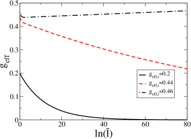
Figure 3: RG flow of $g_{eff}(\bar{l}=\frac{l}{\Lambda_{0}T_{m0}})$ for three different initial conditions $g_{eff,i}=g_{eff}(\bar{l}=1)$ and hence times, and for an initial $\epsilon_{i}=\epsilon(\bar{l}=1)=0.1$. Critical coupling or time is located at $g_{eff,c}=\sqrt{2\epsilon_{i}+\epsilon_{i}^{2}}=0.458$.