Bounces with O(3)$\bm{\times}$O(2) symmetry

Abstract

We study the contribution to the decay of de Sitter vacua from bounces with O(3)$\times$O(2) symmetry. These correspond to the thermal production of a vacuum bubble at the center of a horizon volume with radius $r_{H}$ and a temperature defined by the horizon. They are analogues of the flat spacetime bounces, independent of Euclidean time, that correspond to thermal production of a critical bubble. If either the strength of gravity or the false vacuum energy are increased, with all other parameters held fixed, the bounces approach, and eventually merge with, the Hawking-Moss solution. Increasing the height of the barrier separating the true and false vacuum, and thus the tension in the bubble wall, causes the center of the bubble wall to approach, but never reach, the horizon. This is in contrast with the prediction of the thin-wall approximation, which inevitably breaks down when the wall is near the horizon. Our numerical results show that the Euclidean action of our solutions is always greater than that of the corresponding O(4)-symmetric Coleman-De Luccia bounce.

I Introduction

Vacuum decay by quantum tunneling in curved spacetime was first studied more than thirty years ago by Coleman and De Luccia (CDL) Coleman:1980aw , using a formalism based on bounce solutions of the Euclidean field equations. In recent years there has been renewed interest in this topic, motivated in part by its relevance for a possible string landscape. This has uncovered new aspects of the problem that become significant if the mass scales approach the Planck mass or the bounce radius approaches the horizon length.

It was assumed in Coleman:1980aw that the dominant bounce solution had an O(4) symmetry; we will refer to such solutions as CDL bounces. In this paper we will investigate a different class of solutions, with an ${\rm O(3)}\times{\rm O(2)}$ symmetry, that can occur when the tunneling is from a de Sitter spacetime.

Our motivation for studying these is two-fold. For the case of tunneling in flat spacetime at zero temperature it has been shown that the bounce with minimum action in a theory with a single scalar field has an O(4) symmetry, and it is generally believed that this result extends to theories involving more fields. Indeed, it is quite possible that all bounce solutions in these theories are O(4)-symmetric. No proof of a comparable result in curved spacetime has ever been obtained. The ${\rm O(3)}\times{\rm O(2)}$ symmetry that we impose (which would not be possible in flat spacetime at zero temperature) reduces the field equations for the bounce to a set of ordinary differential equations, thus making the problem quite tractable and allowing comparison of the actions of the two types of bounces.

A second motivation is that these solutions shed light on a reinterpretation of the CDL prescription that was advocated recently by Brown and one of us Brown:2007sd . It was argued there that in the case of decay from a de Sitter vacuum the bounce should be understood as describing tunneling in a finite horizon volume at finite temperature. This has implications for extracting from the bounce the configuration immediately after tunneling. The CDL bounce is topologically a four-sphere, and it is commonly asserted that the configuration after tunneling is obtained from the three-sphere lying on the “equator” of the bounce. By contrast, it was argued in Ref. Brown:2007sd that half of this three-sphere gives the configuration within the horizon volume after tunneling, with the other half giving the configuration before tunneling. The fields beyond the horizon, either before or after tunneling, are never specified and do not enter the calculation. For CDL bounces corresponding to vacuum bubbles much less than horizon size there is little practical difference between the two interpretations. The differences become significant as the bubble approaches horizon size and, especially, in the Hawking-Moss Hawking:1981fz limit. For the bounces we consider, the differences in interpretation are manifest for all bubble sizes. From the viewpoint of Ref. Brown:2007sd these bounces correspond to thermal production of a single bubble, whereas the conventional viewpoint would yield the somewhat surprising conclusion that a pair of bubbles had been produced.

Our interest in this these bounces was first raised by the work of Garriga and Megevand Garriga:2003gv ; Garriga:2004nm . Motivated by the analogy with the thermal production of bubbles in flat spacetime, they studied bounces with ${\rm O(3)}\times{\rm O(2)}$ symmetry and, indeed, did interpret these as corresponding to the nucleation of a pair of bubbles. The discussion was originally in the context of brane nucleation Brown:1987dd ; Brown:1988kg , in which the bubble walls are closed 2-branes, but their analysis can also be applied to field theory nucleation in the thin-wall approximation. We will differ from them in not restricting ourselves to this thin-wall limit. In fact, we will see that the thin-wall approximation inevitably breaks down when the bubble becomes sufficiently large, in what is perhaps the most interesting limit of these solutions.

We work in the context of a scalar field theory with Lagrangian

$${\cal L}=\frac{1}{2}(\partial_{\mu}\phi)^{2}-V(\phi)\,,$$ (1)

where $V(\phi)$ has two local minima, with the higher (lower) being termed the false (true) vacuum. We assume that both minima have positive energy, and are thus de Sitter spacetimes. Although our focus is on the nucleation of a true vacuum bubble in a false vacuum background, we also consider the nucleation of a bubble of false vacuum within a de Sitter true vacuum background. Although this process is energetically forbidden in the absence of gravity, it can occur in de Sitter spacetime with its nonzero temperature $T_{\rm dS}$ Lee:1987qc . In contrast with the CDL case, the bounces governing the nucleation of true vacuum and false vacuum bubbles are not identical.

The remainder of this paper is organized as follows. In Sec. II, we review the essentials of vacuum tunneling, focusing on some features of particular relevance here. In Sec. III, we set up the formalism that we will use, and obtain some basic results concerning our solutions. In Sec. IV we discuss the application of the thin-wall approximation to our problem, explaining how its applicability is more limited than in the case of bounces with O(4) symmetry. We then turn to the description of the ${\rm O(3)}\times{\rm O(2)}$-symmetric bounces themselves. Some limiting cases that can be handled analytically are discussed in Sec. V, and in Sec. VI we describe the results of our numerical solutions. Section VII contains some concluding remarks.

II Review of vacuum tunneling

II.1 Flat spacetime at zero temperature

In flat spacetime at zero temperature, vacuum decay occurs through the production of bubbles of true vacuum via quantum tunneling. Importantly, this is not a tunneling process from homogeneous false vacuum to homogeneous true vacuum, but rather tunneling from an initial configuration that is pure false vacuum to a final configuration containing a bubble of true vacuum (or an approximation thereof) within a false vacuum background. The tunneling is not actually through the one-dimensional barrier that appears in a plot of $V(\phi)$, but rather through an infinite-dimensional barrier in configuration space defined by the potential energy functional

$$U[\phi(x)]=\int d^{3}x\left[\frac{1}{2}({\bm{\nabla}}_{\mu}\phi)^{2}+V(\phi)\right]\,.$$ (2)

One approach to this problem is via the WKB method. With one degree of freedom, $q(t)$, the WKB approximation gives an amplitude for tunneling through a barrier that is proportional to $e^{-{\cal B}}$, where ${\cal B}$ is of the form

$${\cal B}=2\int_{q_{1}}^{q_{2}}dq\sqrt{2[V(q)-E]}$$ (3)

with $V(q_{1})=V(q_{2})=E$. For a barrier in a multidimensional configuration space, one must find a path through the barrier for which the corresponding one-dimensional tunneling exponent ${\cal B}$ is a local minimum Banks:1973ps ; Banks:1974ij . Coleman Coleman:1977py showed that the problem of finding a stationary point of ${\cal B}$ is equivalent to finding a “bounce” solution of the Euclidean equations of motion. In the field theory case, the bounce is a solution $\phi({\bf x},\tau)$ in four-dimensional Euclidean space. The hypersurface at the initial value $\tau_{\rm init}$ (which is equal to $-\infty$ for tunneling from the false vacuum) gives the configuration before tunneling, while the configuration $\phi({\bf x},\tau=0)$ along the hypersurface through the center of the bounce gives the optimal exit point from the potential energy barrier; i.e., the form of the bubble at nucleation. The hypersurfaces at intermediate Euclidean times $-\infty<\tau<0$ give successive configurations along the optimal tunneling path. Those for $0<\tau<\infty$ are simply mirror images of those for negative $\tau$, thus motivating the term “bounce”. The bubble nucleation rate per unit volume is of the form $\Gamma=Ae^{-{\cal B}}$, with ${\cal B}$ being equal to the difference of the Euclidean actions of the bounce and the pure false vacuum.

Subject to only mild assumptions on the potential Coleman:1977th , the bounce of minimum action can be shown to have an O(4) symmetry. This bounce has a central region, in which $\phi$ is close to its true vacuum value, within an infinite region of false vacuum, with the two regions separated by a wall of finite thickness in which $\phi$ traverses the potential barrier, as shown in Fig. 1.

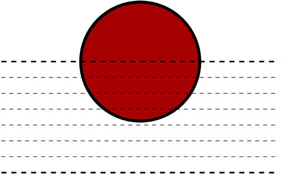
Figure 1: Schematic view of a bounce in flat spacetime. The shaded area is the region of approximately true vacuum, while the heavy circle surrounding it represents the wall region. In actuality, the field is not strictly constant outside the wall, but instead has an exponential tail and only reaches its false vacuum value at infinite distance. The horizontal dashed lines represent a sequence of spatial hypersurfaces of constant $\tau$ that trace out a path in configuration space. The lower heavy dashed line (corresponding to $\tau=-\infty$) indicates the initial pure false vacuum state, while the heavy dashed line through the center of the bounce corresponds to the field configuration at bubble nucleation.

An alternative approach is to use a Euclidean path integral to calculate the imaginary part of the energy of the false vacuum, which is closely related to $\Gamma$ Callan:1977pt . This gives the prefactor $A$ in terms of the eigenvalues of small fluctuations about the bounce, with the imaginary part of the energy emerging from the presence of a single negative eigenvalue. If there are additional negative eigenvalues, the path specified by the bounce is not even a local minimum of ${\cal B}$, but rather a saddle point, and the bounce solution must be discarded Coleman:1987rm .

II.2 Finite temperature

Both the WKB and the path integral approaches show that tunneling at a nonzero temperature $T$ is governed by a bounce solution that is periodic in imaginary time with period $\beta=1/T$. Two types of periodic bounces can be distinguished.

At low temperature the bounce is a somewhat deformed and elongated version of the zero-temperature bounce, with the O(4) symmetry reduced to an O(3) symmetry. Such bounces correspond to thermally assisted tunneling processes in which thermal effects allow the system to start the tunneling at a somewhat higher point on the potential energy barrier. At sufficiently high temperatures this solution may cease to exist.

The second type of solution corresponds to a thermal fluctuation to a saddle point at the top of a “mountain pass” over the potential energy barrier. These solutions are independent of $\tau$. Each three-dimensional spatial slice is infinite in extent and describes an O(3)-symmetric configuration $\phi({\bf x})$ with a central true vacuum bubble of critical size. The Euclidean action of these solutions is equal to the energy of this critical bubble divided by the temperature. Although these solutions exist for all values of $T$, at low temperature they have multiple negative modes and must therefore be discarded. Because this point will be important for us later, let us examine it a bit more closely.

A critical bubble solution $\phi({\bf x})$ is a saddle point of the potential energy functional $U[\phi]$. The second variation of $U$ has a single negative mode $\psi_{-}({\bf x})$ satisfying

$${\delta^{2}U\over\delta\phi^{2}}\,\psi_{-}=-{\bm{\nabla}^{2}}\psi_{-}({\bf x})+V^{\prime\prime}(\phi({\bf x}))\,\psi_{-}({\bf x})=\lambda_{-}\psi_{-}({\bf x})$$ (4)

with $\lambda_{-}=-k^{2}<0$. The second variation of the Euclidean action,

$${\delta^{2}S\over\delta\phi^{2}}=-{d^{2}\over d\tau^{2}}-{\bm{\nabla}^{2}}+V^{\prime\prime}(\phi({\bf x}))\,,$$ (5)

must then have a spectrum that includes eigenmodes of the form

$$\cos\left({2\pi n\tau\over\beta}\right)\psi_{-}({\bf x})\,\qquad n=0,1,\dots$$ (6)

and

$$\sin\left({2\pi n\tau\over\beta}\right)\psi_{-}({\bf x})\,\qquad n=1,2,\dots$$ (7)

with eigenvalues

$$\lambda_{n}=-k^{2}+\left({2\pi n\over\beta}\right)^{2}\,.$$ (8)

Hence, at temperatures $T<k/2\pi$ there are multiple negative modes, and the $\tau$-independent bounce must be discarded. In the flat spacetime thin-wall approximation with a critical bubble of radius $R$ one finds that $k=\sqrt{2}/R$. More generally, we expect that $k\sim 1/{\cal R}$, where ${\cal R}$ is a characteristic length scale of the critical bubble solution. Thus, we must require that

$$T\gtrsim{1\over 2\pi{\cal R}}\,.$$ (9)

II.3 Including gravity

Coleman and De Luccia proposed Coleman:1980aw that the effects of gravity on bubble nucleation could be obtained by including a curvature term in the Euclidean action and seeking a bounce solution that satisfies the coupled Euclidean Einstein and matter equations. If one assumes that the bounce has an O(4) symmetry, and $V(\phi)$ is everywhere positive, the bounce solution is topologically a four-sphere that can be viewed as the hypersurface

$$x_{1}^{2}+x_{2}^{2}+x_{3}^{2}+x_{4}^{2}+x_{5}^{2}=H^{-2}$$ (10)

in a five-dimensional Euclidean space, although not necessarily with the metric implied by the embedding. An O(4)-symmetric solution is obtained by requiring invariance under rotations among the first four coordinates. The scalar field $\phi$ is then a function only of $x_{5}$.

Figure 2 illustrates such a solution for the case where the bubble nucleates with a size much smaller than the false vacuum horizon length $H_{\rm fv}^{-1}$. Analogy with the flat spacetime case illustrated in Fig. 1 might suggest that the configuration after nucleation is given by a slice along the “equator” of this hypersphere that cuts through the center of the true vacuum region, as shown in the figure, with the tunneling path given by a sequence of parallel horizontal slices. This interpretation becomes problematic when the bubble size becomes comparable to the horizon length and there is no plausible candidate for the initial configuration. The is especially so in the limit where the bounce becomes the homogeneous Hawking-Moss solution Hawking:1981fz and a straightforward application of the interpretation would imply that the bounce corresponded to a transition in which all of space fluctuated to $\phi_{\rm top}$, the value at the top of the barrier in $V(\phi)$.

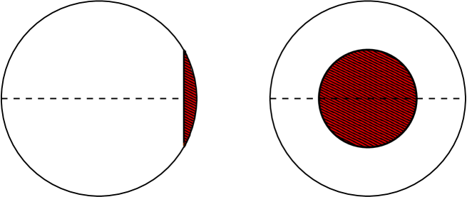
Figure 2: Two views of the CDL bounce. The bounce has the topology of a four-sphere, and is shown here as if embedded in a five-dimensional Euclidean space. Because of the bounce’s O(4) symmetry, the fields and metric have nontrivial dependence only on $x_{5}$. The left-hand view shows the bounce as viewed from a point outside the bounce on an axis perpendicular to the $x_{4}$-$x_{5}$ plane, where $x_{4}$ and $x_{5}$ correspond to the vertical and horizontal directions in the figure, respectively. The shaded area corresponds to the region of approximately true vacuum. The horizontal dashed line has often been taken, by analogy with the heavy dashed line in Fig.1, as giving the configuration at bubble nucleation. The right-hand view shows the bounce as viewed from a point to its right on the positive $x_{5}$-axis. The $x_{4}$ axis again corresponds to the vertical direction, while the horizontal direction now corresponds to an axis perpendicular to the $x_{4}$-$x_{5}$ plane.. A view from a corresponding point on the negative $x_{5}$-axis would show only a region of approximate false vacuum.

In Ref. Brown:2007sd it was argued that one should instead interpret the Coleman-De Luccia formalism as describing thermal tunneling within a horizon volume, with the temperature being the one defined by the horizon. From this viewpoint, the solutions are analogous to those in flat spacetime at finite temperature, but with the crucial difference that the spatial slices of constant Euclidean time are finite in extent. Thus, these solutions exist on a space that is topologically the product of a three-ball (the horizon volume) and a circle (the periodic Euclidean time $\tau$). This suggests a “low-temperature” bounce solution such as that shown in Fig. 3a. The boundary of this space is a family of two-spheres, each labeled by a value of $\tau$.

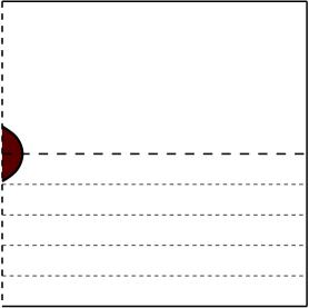
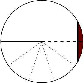
(a)                                                        (b)

Figure 3: The CDL bounce viewed as low-temperature thermal tunneling within a horizon volume. In (a) the horizontal lines represent three-balls with their center on the left and their outer edge, at the horizon, on the right. The horizontal line at the bottom of the figure corresponds to the configuration before tunneling, while the one at the center of the figure corresponds to the configuration after tunneling. As in Fig. 1, the intermediate horizontal lines define the optimum tunneling path through configuration space. In (b) the same CDL solution is represented, but with the path through configuration space defined by a series of radial lines. Again, each of these represents a three-ball, with center of the ball at the edge of the figure and the two-sphere boundary at the horizon at the center of the figure. The initial and final configurations correspond to the left solid and right dashed horizontal radii, respectively.

At first sight, this seems nothing like the CDL bounce. However, this can also be represented as in Fig. 3b, with the hypersurfaces of constant $\tau$ appearing as diagonal sections cutting halfway through a four-sphere. On each section the point at the edge of the diagram corresponds to the center of the horizon volume, while the bounding horizon radius two-sphere appears at the center of the diagram, $x_{4}=x_{5}=0$. Drawn in this manner, the bounce looks like the four-sphere bounce of Fig. 2. It actually is topologically a four-sphere if the two-sphere boundaries of the sections are all identified.

There appears to be no a priori requirement that these two-spheres be identified, nor that the metric should be smooth there if they are identified. Nevertheless, the O(4)-symmetric CDL bounce, with an everywhere smooth metric, can be obtained in this fashion. However, we see that the equatorial slice is now composed of two parts. One half gives the field configuration at the time of bubble nucleation, but only within the horizon volume. The other half gives the field configuration in this horizon volume before the tunneling process. Note that the bounce gives us no information about the field or metric beyond the horizon, other than the fact that they effectively create a thermal bath for the horizon volume.

With this understanding of the CDL bounce as describing low-temperature thermally assisted tunneling, we see that the gravitational analogue of the flat spacetime high-temperature bounce is one that is independent of $\tau$, with the slices of constant $\tau$ describing the critical bubble configuration that is reached by thermal fluctuation. The Hawking-Moss solution is the simplest example, and corresponds to a spatially homogeneous critical “bubble” that fills the horizon volume. However, there can also be critical bubbles that are smaller than horizon size. One such is obtained simply by rotating a CDL bounce so that its symmetry axis is, say, along the $x_{1}$ axis. This rotated bounce corresponds to thermal nucleation of a critical bubble centered at the horizon Brown:2007sd .

We will proceed by seeking a different, and perhaps more obvious, type of bounce, namely one that is independent of $\tau$ and spherically symmetric on each constant-$\tau$ slice. This would correspond to thermal production of a critical bubble located at the center of the horizon volume. Drawn as a four-sphere, the bounce would appear as in Fig. 4. We see here a case where the analysis of Ref. Brown:2007sd leads to a prediction that is clearly different from the conventional interpretation. Whereas the latter would view such bounces as describing the production of a pair of bubbles, under the interpretation of Ref. Brown:2007sd only a single bubble is produced.

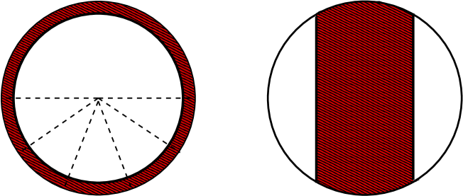
Figure 4: Two views of the O(3)$\times$O(2)-symmetric bounce. These are from the same viewpoints as those of the CDL bounce in Fig. 2. (The view on the right would be the same if viewed from along any axis in the $x_{4}$-$x_{5}$ plane.) On the left-hand view the radial dashed lines correspond to the similar lines in Fig. 3b. The bounce is independent of the Euclidean time, and the three-dimensional configuration corresponding to any one of these lines contains a single true vacuum critical bubble in the center of a false vacuum horizon volume.

III Formalism and some basic results

We are thus led to seek solutions that have nontrivial behavior in three spatial dimensions, but that are constant in Euclidean time. If we impose spherical symmetry on the spatial slices, the metric on the four-dimensional space can be written in the form

$$ds^{2}=B(r)d\tau^{2}+A(r)dr^{2}+r^{2}d\Omega^{2}$$ (11)

and the scalar field $\phi$ is a function only of $r$. Each spatial slice is a three-ball bounded by a two-sphere at $r=r_{H}$, with the horizon radius $r_{H}$ corresponding to a zero of $g^{rr}=1/A$. In order that the metric be nonsingular at $r=0$, we must require that $A(0)=1$. We do not fix $B(0)$ directly, but instead require that it be such that the product $AB$ is equal to unity at the horizon. Generically, there is a region of approximate true vacuum centered around the origin, $r=0$, an outer region of approximate false vacuum extending out to the horizon, and a wall region separating the two.

In the analogous flat spacetime case the temperature, and hence the periodicity, can be chosen arbitrarily, but in our curved spacetime problem we expect the temperature to be specified by the metric. We therefore assume that the periodicity $\beta$ of the Euclidean time is determined by the surface gravity at the horizon of the Lorentzian counterpart of our Euclidean metric; i.e.,

$$\beta={1\over T}=4\pi\left[B^{\prime}\left({1\over A}\right)^{\prime}\right]_{r_{H}}^{-1/2}\,,$$ (12)

where a prime indicates differentiation with respect to $r$ and the subscript indicates that all quantities are to be evaluated at the horizon. Now note that

$$B^{\prime}={d\over dr}\left[(AB)\left({1\over A}\right)\right]=(AB)^{\prime}\,\left({1\over A}\right)+(AB)\,\left({1\over A}\right)^{\prime}\,.$$ (13)

Because $A^{-1}=0$ and $AB=1$ at the horizon, we have $B^{\prime}=(A^{-1})^{\prime}$ at the horizon and

$$\beta=-4\pi[B^{\prime}(r_{H})]^{-1}\,,$$ (14)

with the minus sign arising because $B^{\prime}$ is negative at the horizon. With a uniform vacuum $\beta$ would be $2\pi r_{H}$; for the bounce solutions it remains of this order of magnitude.

With this periodicity, the four-sphere obtained by identifying all of the boundary two-spheres is a smooth manifold, just as in the CDL solution. However, as in the CDL case, we view this as incidental and do not require $\phi$ to be smooth on this two-sphere. Such smoothness would require that $\phi^{\prime}=d\phi/dr$ vanish at $r=r_{H}$. As we will see, this is only possible in the (unattainable) limit in which the thin-wall approximation is exact. Although having $\phi^{\prime}(r_{H})\neq 0$ implies a discontinuity in slope along a path passing through the two-sphere, this discontinuity does not imply any cost in action, and we see no problem with this.

The Euclidean action is

$$S = \int d^{4}x\sqrt{g}\left(-{1\over 16\pi G}R+{\cal L}_{\rm matter}\right)$$ (15)

$$= 4\pi\beta\int_{0}^{r_{H}}dr\,r^{2}\sqrt{AB}\left[-{1\over 16\pi G}R+\frac{1}{2}{(\phi^{\prime})^{2}\over A}+V(\phi)\right]\,.$$ (16)

The curvature scalar that follows from the metric of Eq. (11) is

$$R=-{1\over r^{2}\sqrt{AB}}{d\over dr}\left[r^{2}{B^{\prime}\over\sqrt{AB}}\right]+{2\over r^{2}}{d\over dr}\left[r\left(1-\frac{1}{A}\right)\right]\,.$$ (17)

Substituting this back into the action gives

$$S={\beta\over 4G}\left[r^{2}{B^{\prime}\over\sqrt{AB}}\right]_{r=0}^{r=r_{H}}+4\pi\beta\int_{0}^{r_{H}}dr\,\sqrt{AB}\left\{{1\over 8\pi G}{d\over dr}\left[r\left(\frac{1}{A}-1\right)\right]+r^{2}\left[\frac{1}{2}{(\phi^{\prime})^{2}\over A}+V(\phi)\right]\right\}\,.$$ (18)

Although this is written in terms of the three functions $A(r)$, $B(r)$, and $\phi(r)$, it is more convenient to treat $AB$, rather than $B$, as the independent variable. Varying the action with respect to the independent variables then leads to

$$0 = {1\over 8\pi G}{d\over dr}\left[r\left({1\over A}-1\right)\right]+r^{2}\left[\frac{1}{2}{(\phi^{\prime})^{2}\over A}+V(\phi)\right]\,,$$ (19)

$$0 = {(\sqrt{AB})^{\prime}\over\sqrt{AB}}-4\pi Gr(\phi^{\prime})^{2}\,,$$ (21)

$$0 = {1\over r^{2}\sqrt{AB}}{d\over dr}\left[r^{2}\sqrt{AB}\,{\phi^{\prime}\over A}\right]-{dV\over d\phi}\,.$$ (23)

For any solution of these equations [or even any configuration satisfying Eq. (19)], the integral in Eq.(18) vanishes. Evaluating the first term with the aid of Eq. (14), and recalling our convention that $AB=1$ at the horizon, we obtain

$$S_{\rm bounce}=-{\pi\over G}\,r_{H}^{2}\,.$$ (24)

This agrees with the thin-wall result of Ref. Garriga:2004nm , and could in fact have been anticipated on more general grounds Banados:1993qp ; Hawking:1995fd .

Finally, the exponent in the tunneling rate is the difference between the Euclidean actions of the bounce and of the original false vacuum; i.e.,

$${\cal B}=S_{\rm bounce}-S_{\rm fv}={\pi\over G}(\Lambda^{2}_{\rm fv}-r_{H}^{2})\,,$$ (25)

where the false vacuum horizon radius

$$\Lambda_{\rm fv}=H^{-1}_{\rm fv}=\sqrt{3\over 8\pi GV_{\rm fv}}\,.$$ (26)

For actually seeking bounce solutions, it is convenient to recast our field equations a bit. First, the equations are simplified by defining

$$f=\frac{1}{A}\,.$$ (27)

Equation (19) then becomes

$$0={1\over 8\pi G}{d\over dr}\left[r(f-1)\right]+r^{2}\left[\frac{1}{2}(\phi^{\prime})^{2}f+V(\phi)\right]\,.$$ (28)

If we define a mass ${\cal M}(r)$ by

$$f(r)=1-{2G{\cal M}(r)\over r}\,,$$ (29)

this can be rewritten as

$${\cal M}^{\prime}=4\pi r^{2}\left[\frac{1}{2}(\phi^{\prime})^{2}f+V(\phi)\right]\,.$$ (30)

Second, we note that substitution of Eq. (21) into Eq. (23) gives

$$0=f\left[\phi^{\prime\prime}+\frac{2}{r}\,\phi^{\prime}+4\pi Gr(\phi^{\prime})^{3}\right]+f^{\prime}\phi^{\prime}-{dV\over d\phi}\,.$$ (31)

This and Eq. (30) give a pair of equations involving only $f$ and $\phi$. Once these have been solved, $AB$ is readily obtained by integrating Eq. (21). With our convention that $AB$ be equal to unity at the horizon, this gives

$$A(r)B(r)=\exp\left[-8\pi G\int_{r}^{r_{H}}dr^{\prime}\,r^{\prime}\,(\phi^{\prime})^{2}\right]\,.$$ (32)

We must now determine the boundary conditions. We clearly need to avoid singularities at the center of the bounce, $r=0$. This leads to the requirements

$$f(0) = 1\,,$$ (33)

$$\phi^{\prime}(0) = 0\,.$$ (34)

The value of $\phi(0)$ is not predetermined, although it must be on the side of the barrier corresponding to the new vacuum (i.e., the true vacuum side for the case of false vacuum decay by bubble nucleation).

The horizon is determined by the requirement that $f(r_{H})=0$. Our prescription for specifying the temperature guarantees that the Euclidean metric is nonsingular at $r_{H}$, even when the bounce is viewed as a topological four-sphere and not simply as the product of a three-ball and a circle. In order for $\phi$ to also be nonsingular on the four-sphere we would have to require that $\phi^{\prime}(r_{H})=0$. Equation (31) shows that this implies that $dV/d\phi=0$ at the horizon, which in turn means that the field must be precisely at a vacuum value (or else exactly at the top of the barrier, as in the Hawking-Moss solution). For a nontrivial bounce this is only possible in the limit where the thin-wall approximation is exact.

However, there is no reason to require such smoothness on the four-sphere. Instead, the only requirement is that following from Eq. (31), which implies that

$$0=\left.\left[f^{\prime}\phi^{\prime}-{dV\over d\phi}\right]\right|_{r=r_{H}}$$ (35)

if $\phi^{\prime}$ and $\phi^{\prime\prime}$ remain finite as $r\rightarrow r_{H}$. [In fact, the condition holds even for singular $\phi^{\prime}$, provided that $\phi^{\prime}$ grows more slowly than $(r_{H}-r)^{1/2}$ as the horizon is approached. Note that such a divergence does not imply a divergent action density, and in fact is consistent with a finite derivative of $\phi$ with respect to proper distance from the horizon.]

IV The thin-wall approximation

The thin-wall approximation is often useful for gaining an intuitive understanding of tunneling problems. In this approximation, the bounce is approximated as a region of pure true vacuum surrounded by a region of pure false vacuum, with the variation of the scalar field confined to a thin wall separating the two. There are two essential requirements for this approximation to be valid. First, the thickness of the wall must be much less than the radius of the true vacuum region, so that the wall can be locally approximated as being planar. The second concerns the position dependence of the surface tension $\sigma$ of the wall. Although $\sigma$ was independent of position in most previous tunneling calculations, position dependence is possible. However, for the thin-wall approximation to be reliable, the variation of $\sigma$ must be small on distance scales comparable to the width of the wall.

In flat spacetime the thickness of the wall is determined primarily by the form of the potential barrier separating the true and false vacua. Reducing $\epsilon$, the difference in the energy densities of the two vacua, while keeping the shape of the potential barrier otherwise fixed increases the radius of the true vacuum region. By making $\epsilon$ sufficiently small one can always reach the regime where the thin-wall approximation is valid. This is the case both for O(4)-symmetric zero-temperature bounces and for high-temperature solutions that describe a critical bubble in three dimensions.

With gravity included, the situation is more complicated. Because the false vacuum horizon length limits the size of the bounce, the true vacuum region cannot be made arbitrarily large. To even have a possibility of the thin-wall approximation being valid, the shape of the potential barrier must be such that the natural width of the wall is small compared to the horizon length. If this is the case, then an appropriate reduction of $\epsilon$ can ensure the validity of the approximation for the O(4)-symmetric bounces.

This turns out to not be true for our O(3)$\times$O(2)-symmetric bounces. To understand this, let us begin by assuming that the variations in the metric functions $f$ and $B$ as one passes through the wall are small enough that they can be treated as constants there. Equation (31) then reduces to

$$0=f\left(\phi^{\prime\prime}+\frac{2}{r}\phi^{\prime}\right)-{dV\over d\phi}\,.$$ (36)

If $f$ is treated as a constant near the wall, this is identical with the analogous flat spacetime equation, except for a rescaling $r\rightarrow\tilde{r}=r/\sqrt{f}$. In other words, the wall thickness, measured in terms of $r$, is reduced by a factor of $\sqrt{f}$ compared to the flat spacetime case; this is to be expected, since it is $\tilde{r}$ that measures the proper distance across the wall. Now let us further assume that the second, $2\phi^{\prime}/r$, term can be neglected. Multiplying the above equation by $\phi^{\prime}$ then leads to

$$0={d\over dr}\left[\frac{1}{2}(\phi^{\prime})^{2}f-V(\phi)\right]$$ (37)

so that the quantity in brackets is constant through the wall. Evaluating this constant just outside the wall tells us that in the wall

$$\sqrt{f}\,\phi^{\prime}=\sqrt{2[V(\phi)-V_{\rm fv}]}\,.$$ (38)

Furthermore, we have

$$\int_{\rm wall}dr\,{f\over 2}(\phi^{\prime})^{2} = \int_{\rm wall}dr\,[V(\phi)-V_{\rm fv}]=\int_{\phi_{\rm tv}}^{\phi_{\rm fv}}{d\phi\over\phi^{\prime}}\,{f\over 2}(\phi^{\prime})^{2}$$ (39)

$$= {\sqrt{f}\over 2}\int_{\phi_{\rm tv}}^{\phi_{\rm fv}}d\phi\sqrt{2[V(\phi)-V_{\rm fv}]}$$ (40)

where the integrals over $r$ are restricted to the wall region.

We can therefore define a surface tension

$$\sigma=\int_{\phi_{\rm tv}}^{\phi_{\rm fv}}d\phi\sqrt{2[V(\phi)-V_{\rm fv}]}$$ (41)

and write the contribution to the action from the matter in the wall as

$$4\pi\beta\int_{\rm wall}dr\,r^{2}\sqrt{AB}\left[{f\over 2}(\phi^{\prime})^{2}+V(\phi)-V_{\rm fv}\right]=4\pi R^{2}\beta\sqrt{f}\sqrt{AB}\,\sigma\,.$$ (42)

After the gravitational contribution to the wall action is included, Eq. (42) agrees with the corresponding expression in Ref. Garriga:2004nm , verifying that the surface tension that we have defined in Eq. (41) corresponds to that used in the latter paper.

We must now go back and examine the validity of the assumptions that we have made. In particular, we must show that the fractional changes in $r$, $f$, and $AB$ as one goes through the wall are all small. For the first of these, we note that the thickness of the wall is

$$\Delta r=\sqrt{f}\int_{\phi_{\rm tv}}^{\phi_{\rm fv}}{d\phi\over\sqrt{2[V(\phi)-V_{\rm fv}]}}\,.$$ (43)

Just as in flat spacetime, this can be made arbitrarily small, without materially changing $\sigma$, by making the potential barrier higher by a factor $\gamma^{2}>1$ and narrower by a factor $1/\gamma$. Also, for fixed barrier height and width this expression decreases as one moves toward the horizon.

Equation (32) shows that the fractional change in $AB$ is

$${\Delta(AB)\over AB}=8\pi Gr\int_{\rm wall}dr\,{(\phi^{\prime})^{2}}=8\pi Gr\sigma/\sqrt{f}\,.$$ (44)

From Eqs. (29) and (30) we find that

$$\Delta f = -{2G\over r}\Delta{\cal M}=-{8\pi Gr}\int_{\rm wall}dr\left[\frac{1}{2}f(\phi^{\prime})^{2}+V\right]$$ (45)

$$= -8\pi Gr\left(\sigma\sqrt{f}+V_{\rm fv}\Delta r\right)\,.$$ (46)

Requiring that the fractional changes in $AB$ and in $f$ be small gives the constraint,

$$8\pi Gr\sigma\ll\sqrt{f}<1\,.$$ (47)

This will certainly fail if the bubble wall is too close to the horizon, where $f$ vanishes. In particular, the limiting surface tension $\sigma_{N}$ that is discussed in Ref. Garriga:2004nm does not satisfy Eq. (47). In the field theory context, if the potential is such that Eq. (41) implies $\sigma\gtrsim\sigma_{N}$, then the thin-wall approximation is not valid.

V Limiting cases

Before we turn to our numerical results, it may be helpful to consider some limiting cases.

V.1 Weak gravity

Let us begin by focusing on the effect of varying $G$, with all other parameters held fixed. We first consider the case where $G$ tends toward zero, so that gravitational effects would be expected to be small. If $G$ is sufficiently small, $\phi$ varies from a value near the true vacuum to one exponentially close to $\phi_{\rm fv}$ in an interval $0\leq r\leq\tilde{r}$, where $\tilde{r}$ is much less than $\Lambda_{\rm fv}$. In this region Eq. (31) is well approximated by the corresponding flat spacetime equation. Outside this region, integration of Eq. (30) gives

$${\cal M}(r)=E_{\rm flat}+{1\over 2G}\,{r^{3}\over\Lambda_{\rm fv}^{2}}\,,$$ (48)

where $E_{\rm flat}$ is the energy of the critical bubble in flat spacetime. To leading order the horizon, where $f$ vanishes, is at $r_{H}=\Lambda_{\rm fv}-GE_{\rm flat}$. The tunneling exponent, Eq. (25), is given by

$${\cal B}=2\pi\Lambda_{\rm fv}E_{\rm flat}=E_{\rm flat}/T_{\rm dS}\,,$$ (49)

where $T_{\rm dS}=1/2\pi\Lambda_{\rm fv}$ is the de Sitter temperature of the false vacuum. As expected, this is the Boltzmann exponent one would obtain for nucleation of a critical bubble in flat spacetime at a temperature $T=T_{\rm dS}$. However, because $T\ll 1/\tilde{r}$, the high temperature bounce has multiple negative modes, and must therefore be discarded.

V.2 Strong gravity

Now consider the opposite limit, with $G$ becoming large while all other parameters are held fixed. In this limit $\Lambda_{\rm fv}$ decreases, leaving less and less space for the wall separating the two vacua. As $\Lambda_{\rm fv}$ becomes smaller than the natural width of the wall, $\phi$ is restricted to an increasingly narrow range of values around the top of the barrier. Eventually, the solution becomes spatially homogeneous, with $\phi=\phi_{\rm top}$ everywhere. This is, in fact, the usual Hawking-Moss solution, whose O(5) symmetry has both O(4) and O(3)$\times$O(2) symmetries as subgroups.

The approach to the Hawking-Moss solution can be studied by taking $\delta\phi\equiv\phi_{\rm top}-\phi$ to be small. This quantity enters quadratically in the equations for the metric functions, Eqs.(19) and (21), so to leading order we can linearize the scalar field Eq. (23) in $\delta\phi$ and take the metric functions to be those of a de Sitter spacetime with $V=V(\phi_{\rm top})$. The analysis is then quite analogous to the four-dimensional case that was considered in Ref. Hackworth:2004xb , with the main difference being the replacement of Gegenbauer functions by Legendre functions. We find that the nontrivial bounce solution goes over to the Hawking-Moss solution when

$${V^{\prime\prime}(\phi_{\rm top})\over H_{\rm top}^{2}}\leq 10\,.$$ (50)

V.3 Large vacuum energy

Another possibility is to keep $G$ fixed, but to raise the vacuum energies by adding a large constant to $V(\phi)$. On a pure vacuum solution increasing the vacuum energy has the same effect on the metric as increasing $G$. We would expect the same to be true if the variation of $V(\phi)$ in the region between the two vacua is small compared to the absolute magnitude of the potential. As in the previous case, the bounce solution should go over to the Hawking-Moss solution when Eq. (50) is satisfied.

VI Numerical results

To explore the properties of the bounces more closely, we considered a theory with a quartic potential with two minima. By shifting the zero of $\phi$ so that the minima are equally spaced about the origin, with $\phi_{\rm tv}=v$ and $\phi_{\rm fv}=-v$, any such potential can be brought into the form

$$V(\phi)=\lambda\left(C_{0}v^{4}-kv^{3}\phi-\frac{1}{2}v^{2}\phi^{2}+{k\over 3}v\phi^{3}+\frac{1}{4}\phi^{4}\right)\,.$$ (51)

with $0<k<1$. The top of the barrier separating the two vacua is at $\phi=-kv$. The theory is thus characterized by four dimensionless quantities: $\lambda$, $C_{0}$, $k$, and

$$h=8\pi Gv^{2}\,.$$ (52)

The dependence on one of these, $\lambda$, is rather simple. If $\phi(x)=g(x)$ is a bounce solution for a given value of $\lambda$, then $\phi(x)=g(\gamma x)$ is a solution for the theory with $\lambda$ replaced by $\gamma^{2}\lambda$. The action of the bounce in the latter theory is $\gamma^{-2}$ times that of the original bounce. Thus, the classical solutions have a nontrivial dependence on only the three remaining dimensionless parameters. At the same time, it must be remembered that the validity of the semiclassical method requires that we be in the weak coupling regime $\lambda\ll 1$.

We will find it useful to work with an alternative set of parameters,

$$\epsilon = {1\over v^{4}}(V_{\rm fv}-V_{\rm tv})=\frac{4}{3}\lambda k\,,$$ (53)

$$\alpha = {1\over v^{4}}(V_{\rm top}-V_{\rm fv})={\lambda\over 12}(3-k)(1+k)^{3}\,,$$ (55)

$$U_{0} = {1\over v^{4}}V_{\rm fv}=\lambda\left(-\frac{1}{2}+{2k\over 3}+C_{0}\right)\,,$$ (57)

that characterize the splitting of the vacuum energies, the height of the potential barrier, and the overall magnitude of the vacuum energy. In order to understand the dependence on these features of the potential, we will hold two of these (and $h$) fixed while varying the third. Such a variation corresponds to a more complicated path in the $\lambda$-$C_{0}$-$k$ space, and may extend into the large $\lambda$ strong coupling regime. This does not matter for our purposes, since any such strong-coupling solution is related to a weak-coupling solution whose field and metric profiles differ from the original only by a rescaling of distance

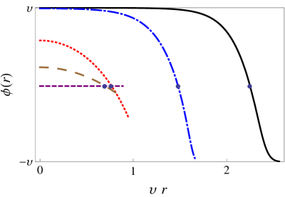
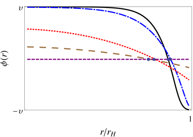
(a)                                                                   (b)

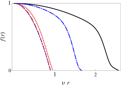
(c)

Figure 5: Evolution of the bounce as the gravitational constant is varied. The first two panels show $\phi$ as a function of (a) $r$ and (b) $r/r_{H}$. In both cases the black dot indicates the value at the top of the barrier. The third panel shows $f=1/A$ as a function of $r$. Reading from left to right, the short-dashed purple, long-dashed brown, dotted red, dot-dashed blue, and solid black lines correspond to $8\pi Gv^{2}$ equal to 0.711, 0.704, 0.628, 0.251, and 0.126. In all cases $U_{0}=2$, $\alpha=3$, and $\epsilon=0.3$.

We have numerically solved the bounce equations for a variety of values of the parameters. Figure 5 shows the effect of varying $G$ with the other parameters held fixed. The horizon radius decreases as gravity is made stronger, just as one would expect. For sufficiently strong gravity, the starting and ending points of the field move significantly away from their respective vacuum values. The solution eventually approaches the Hawking-Moss solution, with $\phi$ being constant and $f$ precisely of the de Sitter form, in agreement with the arguments that we presented in Sec. V. The Hawking-Moss solution is reached at the value predicted by Eq. (50).

We also argued in Sec. V that the effect of uniformly increasing $V_{\rm fv}$ should be qualitatively similar to that of increasing the strength of gravity. This is verified by our numerical solutions, which closely resemble those shown in Fig. 5. Again, the Hawking-Moss solution is reached at the value predicted by Eq. (50).

Figure 6 shows the effect of varying $\epsilon$, the dimensionless difference of the two vacuum energy densities. We see that decreasing $\epsilon$ increases the bubble radius. This behavior is already familiar from the flat spacetime case, where the increased radius is needed for the outward pressure of the interior true vacuum to be able to overcome the surface tension of the bubble wall. Note, though, that we have included a curve for $\epsilon=0$, corresponding to degenerate vacua, and that the outermost curve is for negative $\epsilon$; i.e., the case of a false vacuum bubble forming within a true vacuum region. Neither of these would be possible in flat spacetime, where the bubble radius tends to infinity as $\epsilon$ is taken to zero, and where a true vacuum region cannot nucleate false vacuum bubbles. This is not so when gravitational effects are included. If the true and false vacua are both de Sitter, it is possible to “tunnel upward” from true vacuum to false Lee:1987qc . Although the surface tension and the vacuum pressure would both tend to collapse the resulting bubble, the Hubble flow of de Sitter spacetime overcomes these if the initial bubble size is sufficiently large.

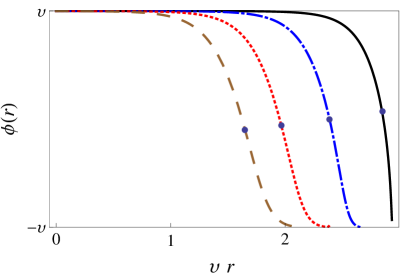
(a)                                                                   (b)

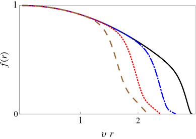
(c)

Figure 6: Behavior of the bounce as $\epsilon$ is varied. Again, panels (a) and (b) show $\phi$ as a function of $r$ and of $r/r_{H}$, with the black dot indicating the value at the top of the barrier. Panel (c) shows the metric function $f=1/A$. Reading from left to right, the dashed brown, dotted red, dot-dashed blue, and solid black lines correspond to $\epsilon$ equal to 2, 1, 0, and $-1$. For all cases $U_{0}=2$, $\alpha=3$, and $8\pi Gv^{2}=0.126$.

In the CDL ansatz, the “new vacuum” region of the bounce is centered about the “North Pole” of the four-sphere, and the “old vacuum” region about the “South Pole”. Nucleation of a bubble of false vacuum rather than true is described by the same bounce solution, but with the labeling of the two poles simply interchanged. Matters are different for the O(3)$\times$O(2)-symmetric bubbles. The spacelike slices of these are three-balls, with the new vacuum near the center and the old vacuum at the outer edge. There is no longer a symmetry between the two regions, and the bounce profiles for the two processes differ, as can be seen in the figure.

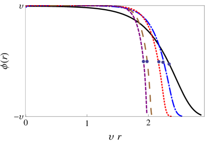
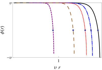
(a)                                                                   (b)

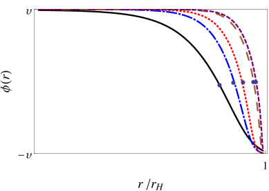
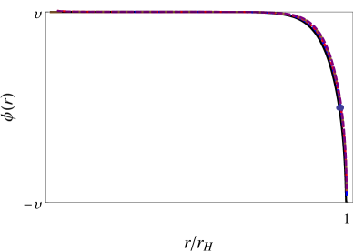
(c)                                                                   (d)

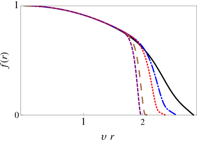
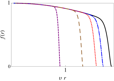
(e)                                                                   (f)

Figure 7: Variation of the bounce with barrier height. The panels on the left correspond to smaller values of $\alpha$, with the short-dashed purple, long-dashed brown, dotted red, dot-dashed blue, and solid black lines corresponding to $\alpha$ equal to 1, 3, 5, 12, and 15. The right-hand panels correspond to larger values of $\alpha$, with the short-dashed purple, long-dashed brown, dotted red, dot-dashed blue, and solid black lines corresponding to $\alpha$ equal to 15, 20, 25, 40, and 100. For all of these $U_{0}=2$, $\epsilon=0.3$, and $8\pi Gv^{2}=0.126$. As in the previous figures, the black dot indicates the value of the field at the top of the barrier.

Perhaps the most interesting behavior is that which occurs when we vary $\alpha$, the parameter characterizing the barrier height in the potential. Increasing the barrier height increases the surface tension in the bubble wall. In flat spacetime this, in turn, requires that the bubble nucleate with a larger radius. A second effect of the increased barrier height is that the bubble wall gets thinner.

Figure 7 shows the effects of varying $\alpha$ on the O(3)$\times$O(2)-symmetric bounces. We see two distinct types of behavior. For smaller values of $\alpha$, illustrated in the panels on the left, the scalar field starts close to the true vacuum value at $r=0$ and then comes exponentially close to the false vacuum by the time that the horizon is reached. In contrast with flat spacetime, the radius at nucleation decreases as $\alpha$ increases. This is largely due to the fact that the increased tension in the bubble wall causes the metric coefficient $f$ to turn over sooner, leading to a smaller horizon radius. However, when the field profile is viewed as a function of $r/r_{H}$, the result is closer to what the flat spacetime experience would have led us to expect. Whether viewed as a function of $r$ or of $r/r_{H}$, the bubble wall becomes thinner and steeper with increasing $\alpha$.

Viewing these results for small $\alpha$, one might be led to expect that further increases in $\alpha$ would lead to an even steeper profile that pushed ever closer to the horizon, perhaps becoming a step function, with an infinitely thin bubble wall, for sufficiently large $\alpha$. This is not what happens. Instead, the value of the field at the horizon, $\phi(r_{H})$, falls visibly short of the false vacuum by an amount that increases with $\alpha$. [For the highest value of $\alpha$ shown here, $\phi(r_{H})=-.85v$.] Furthermore, the wall does not become thinner. Indeed, when plotted as functions of $r/r_{H}$, the various large-$\alpha$ field profiles are almost indistinguishable.

VII Discussion and concluding remarks

We have studied a class of bounce solutions with O(3)$\times$O(2) symmetry. These are curved spacetime analogues of the flat spacetime bounces describing thermal nucleation of critical bubbles. Following the interpretation of Ref. Brown:2007sd , the critical bubble configuration is obtained by taking a constant $\tau$ slice through the bounce. This slice is topologically a three-ball, and gives the scalar field and metric on a horizon volume. No reference is made to quantities beyond the horizon, and the end result of the process is the creation of one bubble, not two.

Using a general quartic potential as an example, we have explored the behavior of the bounces in various regions of parameter space. Either increasing Newton’s constant or raising $V(\phi)$ by a uniform constant, with the shape of the potential otherwise held fixed, drives the bounce toward, and eventually merges it with, the Hawking-Moss solution. Decreasing the energy difference between the new true vacuum and the background false vacuum tends to increase the bubble radius at nucleation, but the effect is hardly as dramatic as in flat spacetime, even in the case where $\epsilon$ changes sign so that the bounce is actually describing the nucleation of a false vacuum bubble in a region of true vacuum.

The effect of increasing the surface tension in the bubble wall by raising the potential barrier is particularly notable. Initially, this makes the bubble wall thinner and moves it closer to the horizon. This fits one’s expectations from the behavior of the thin-wall analysis of Garriga and Megevand Garriga:2003gv ; Garriga:2004nm . However, with further increases the two analyses diverge. In the thin-wall/membrane case the bubble wall reaches the horizon at a critical surface tension $\sigma_{N}$. By contrast, in our field theory case the field profile at the bubble wall asymptotes toward one with nonzero thickness, and in fact shows little variation with increased surface tension.

To be relevant for tunneling, it is not sufficient that the bounce be a solution of the Euclidean field equations. In addition, the spectrum of fluctuations about the bounce must include one negative mode, to give an imaginary part to the energy of the false vacuum, but no more, since additional negative modes would signal that the bounce corresponded to a path that was not a local minimum of the tunneling exponent. There are potentially three types of negative modes for the O(3)$\times$O(2) symmetric solutions. Two of these are closely analogous to the ones associated with thermal bounces in flat spacetime. The first is a mode that is independent of the Euclidean time and corresponds to the radial expansion or contraction of the critical bubble profile. We expect that this negative mode will always be present. The second class of modes are obtained by modulating the amplitude of the previous mode with a sinusoidal variation in the imaginary time. By analogy with the discussion in Sec. II.2, we expect these additional modes to be present if the ratio of the bubble radius to the inverse temperature is too low. In order to avoid these, the bubble radius should be comparable to $r_{H}$.

The third type of negative mode is closely tied to the four-sphere topology of the bounce. It is perhaps easiest to visualize in the limit where the bubble radius is much less than the horizon radius. In this limit the shaded region in Fig. 4 becomes a narrow band stretched along the circumference of the bounce. Moving this true vacuum region to either side reduces its length in the $\tau$ direction and therefore reduces its action. This mode may be avoided if the bubble radius is much larger and the bubble wall is no longer thin but instead has a tail extending out toward the horizon. This is the same region of parameter space as is required to avoid additional negative modes of the second type.

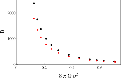
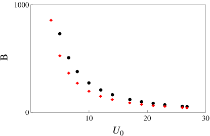
(a)                                                                   (b)

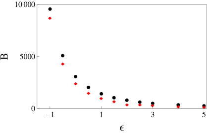
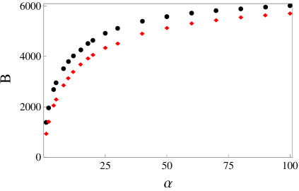
(c)                                                                   (d)

Figure 8: Comparison of the tunneling exponents for the CDL bounce (red diamonds) and the O(3)$\times$O(2)-symmetric bounce (black circles) as one parameter is varied with the other three held fixed. When held fixed, $U_{0}=2$, $\alpha=3$, $\epsilon=0.3$, and $8\pi Gv^{2}=0.126$.

Finally, even if the O(3)$\times$O(2)-symmetric bounce has only a single negative mode, it is of practical relevance only if its action is less than that of the CDL bounce. Indeed, one of the goals of our investigation was to test the conjecture that the bounce with minimum action has O(4) symmetry. It was already shown in Ref. Garriga:2004nm that in the thin-wall approximation the O(3)$\times$O(2)-symmetric bounce always has a higher action than the corresponding CDL action. Our numerical methods allow us explore the much larger parameter space that is allowed when one goes beyond this approximation. The results are summarized in Fig. 8. Each of the four panels corresponds to a one-dimensional path through this parameter space. We see that the tunneling exponent for the O(3)$\times$O(2) is never less than that of the CDL bounce. The two approach and become equal at large values of $G$ and of $U_{0}$. This can be understood by recalling that the O(3)$\times$O(2)-symmetric bounce reduces to the Hawking-Moss solution when $V^{\prime\prime}/H^{2}\leq 10$ at the top of the barrier [see Eq. (50)]. For $4<V^{\prime\prime}/H^{2}\leq 10$ there is always a CDL bounce whose action is less than that of the Hawking-Moss solution, but at $V^{\prime\prime}/H^{2}=4$ the CDL solution merges into the Hawking-Moss.

These numerical tests are, of course, not conclusive. Although we have no reason to expect it, there could be unexplored regions of our parameter space where the action is less than the CDL action. More generally, there may be other choices of the potential for which the CDL bounce is not optimal. Conclusive analytical results on this issue would be welcome.

- (1) S. Coleman and F. De Luccia, Phys. Rev. D 21, 3305 (1980).
- (2) A. R. Brown and E. J. Weinberg, Phys. Rev. D 76, 064003 (2007).
- (3) S. W. Hawking and I. G. Moss, Phys. Lett. B 110, 35 (1982).
- (4) J. Garriga and A. Megevand, Phys. Rev. D 69, 083510 (2004).
- (5) J. Garriga and A. Megevand, Int. J. Theor. Phys. 43, 883 (2004).
- (6) J. D. Brown and C. Teitelboim, Phys. Lett. B 195, 177 (1987).
- (7) J. D. Brown and C. Teitelboim, Nucl. Phys. B 297, 787 (1988).
- (8) K. Lee and E. J. Weinberg, Phys. Rev. D 36, 1088 (1987).
- (9) T. Banks, C. M. Bender, and T. T. Wu, Phys. Rev. D8, 3346.
- (10) T. Banks and C. M. Bender, Phys. Rev. D8, 3366 (1973).
- (11) S. Coleman, Phys. Rev. D15, 2929-2936 (1977).
- (12) S. Coleman, V. Glaser, and A. Martin, Commun. Math. Phys. 58, 211 (1978).
- (13) C. G. Callan and S. Coleman, Phys. Rev. D16, 1762-1768 (1977).
- (14) S. Coleman, Nucl. Phys. B298, 178 (1988).
- (15) M. Banados, C. Teitelboim and J. Zanelli, Phys. Rev. Lett. 72, 957 (1994).
- (16) S. W. Hawking and G. T. Horowitz, Class. Quant. Grav. 13, 1487 (1996).
- (17) J. C. Hackworth and E. J. Weinberg, Phys. Rev. D 71, 044014 (2005).