Luminosity distance in Swiss cheese cosmology with randomized voids and galaxy halos

Abstract

We study the fluctuations in luminosity distance due to gravitational lensing produced both by galaxy halos and large scale voids. Voids are represented via a “Swiss cheese” model consisting of a $\Lambda$CDM Friedman-Robertson-Walker background in which a number of randomly distributed, spherical regions of comoving radius 35 Mpc are removed. A fraction of the removed mass is then placed on the shells of the spheres, in the form of randomly located halos, modeled with Navarro–Frenk–White profiles. The remaining mass is placed in the interior of the spheres, either smoothly distributed, or as randomly located halos. We compute the distribution of magnitude shifts using a variant of the method of Holz & Wald (1998), which includes the effect of lensing shear. In the two models we consider, the standard deviation of this distribution is 0.065 and 0.072 magnitudes and the mean is -0.0010 and -0.0013 magnitudes, for voids of radius 35 Mpc, sources at redshift 1.5, with the voids chosen so that 90% of the mass is on the shell today. The standard deviation due to voids and halos is a factor $\sim 3$ larger than that due to 35 Mpc voids alone with a 1 Mpc shell thickness which we studied in our previous work. We also study the effect of the existence of evacuated voids, by comparing to a model where all the halos are randomly distributed in the interior of the sphere with none on its surface. This does not significantly change the variance but does significantly change the demagnification tail. To a good approximation, the variance of the distribution depends only on the mean column depth and concentration of halos and on the fraction of the mass density that is in the form of halos (as opposed to smoothly distributed): it is independent of how the halos are distributed in space. We derive an approximate analytic formula for the variance that agrees with our numerical results to $\lesssim 20\%$ out to $z\simeq 1.5$.

I Introduction

I.1 Background and Overview

A number of surveys are being planned to determine luminosity distances to various different astronomical sources, and to use them to constrain properties of the dark energy or modification to gravity that drives the cosmic acceleration. Perturbations to luminosity distances due to gravitational lensing by large scale and galaxy scale structures are a source of error for these studies, see, e.g., Refs p3Ref1 ; p3Ref2 ; p3Ref3 ; p3Ref4 ; p3Ref5 ; p3Ref6 .

In this paper we use the computational method developed in Ref. p3Ref1 to study the effect of density inhomogeneities on luminosity distances in two idealized “Swiss cheese” models p3Ref3 ; p3Ref7 ; p3Ref8 ; p3Ref9 ; p3Ref10 of large scale ($\sim 30$ Mpc) and galaxy scale structures. Our models seek to capture the property that most of the matter is concentrated in galaxy halos on the outer edges of voids while the void interiors are relatively sparse. Our first model is an extension of our previous work p3Ref1 where we idealize the interior of a spherical void as a uniform underdense region and the surface of the sphere contains a randomized distribution of galaxy halos with Navarro–Frenk–White (NFW) profiles p3Ref13 . Our second model retains the randomly distributed galaxy halos on the surface of the voids, and replaces the interior uniform density with randomly distributed galaxy halos with NFW profiles. In both models we keep fixed the parameters of the voids and halos. Even though neither of these models represent realistic matter distributions within a void, they should capture the main qualitative features of lensing.

I.2 Summary of Computation and Results

In Section II, we give a detailed description of the NFW halo density profile that we adopt which is motivated by observations. We also describe our two models of the entire distribution of matter, including both large scale void structures and smaller scale halo structures.

In Section III, we review the method we use to compute the distribution of lensing magnifications. We then describe how to compute the lensing convergence for a single halo. We compare our numerical results for the distribution of magnifications with analytic expressions. We also estimate the number of realizations required to get a reasonable accuracy in the computed distribution of magnifications (e.g, obtain the mean of the distribution to an accuracy of $<1\%$ ). The accuracy of the numerical results scales as $N^{-1/2}$ as expected, where $N$ is the number of realizations.

In Section IV, we study our first Swiss cheese model. We start by describing the model, and study the propagation of light rays through just a single void. Then, we derive analytic results for the magnification and use these to check our numerical results. We study the expected number of halo intersections, the redshift dependence of the magnification distribution, and determine the contribution of shear to our results. We note that the standard deviation is $\sim 3$ times larger than that due to voids with no halos, specifically the model of p3Ref1 consisting of voids of radius 35 Mpc with smooth underdense interiors and a smooth overdensity concentrated on the surface of the sphere with a thickness of 1 Mpc. We show that the redshift dependence of the mean and standard deviation agrees with analytic results to $<10\%$. We also note that the standard deviation changes by less than $3\%$ if shear is neglected (see Section IV C below).

One effect which our models do not include is the clustering of halos, that is, the correlations between the locations of different halos. While it would be more realistic to include the effects of clustering, our simplified models should capture the essence of the effects of large scale inhomogeneities.

In Section V, we study the second Swiss cheese model. Again, we first describe the model and study just a single void. We derive analytic results for the lensing convergences and use these to check our numerical results. There is a higher probability of demagnification; this shift is expected because the density contrast inside the void is now sharper because it is empty (with a smattering of a small number of halos) whereas the first model has a smooth interior matter distribution. The redshift dependence of the mean and standard deviation of the second model are similar to those of the first model. In the two models we consider, the standard deviations of this distribution are 0.065 and 0.072 magnitudes and the means are -0.0010 and -0.0013 magnitudes, for voids of radius 35 Mpc, sources at redshift 1.5, with the voids chosen so that 90% of the mass is on the shell today. We compare the distributions for configurations with and without voids for a source at $z_{s}=1.5$. We find that the voids do not significantly change the variance but do significantly change the demagnification tail and the mode.

We find that since the distribution is skewed, the mode is positive, while the variance is determined primarily by rays that intersect halos. The scale of the voids does not significantly influence our results. The main parameters that determine the mode and variance of the distribution is the mean column depth and concentration of halos and the fraction of the mass density that is in the form of halos (as opposed to smoothly distributed). The distribution of halos in space (i.e., in the interior versus the surface) is unimportant. Hence, our models bracket the range of possibilities of magnifications. Our analysis is generally consistent with other analytic and computational results p3Ref14 ; p3Ref15 ; p3Ref16 ; p3Ref17 ; p3Ref18 ; p3Ref19 ; p3Ref20 ; p3Ref21 ; p3Ref22 . We also compare our results to those of Kainulainen & Marra p3Ref11 ; p3Ref12 who use a similar but slightly different simplified model of large scale structure.

II Model of Lensing Due to Galaxy halos and Voids

II.1 Galaxy halo profile

We model the galaxy halos with an NFW profile p3Ref13 , with a density distribution

$$\rho_{\mathrm{halo}}\left(r\right)=\left\{\begin{array}[]{c}0\;\;\;\;\;\;\;\;\;\;\;\;\;\;r\geqslant CR_{s}\\ \frac{\rho_{0}R_{{\rm s}}^{3}}{r\left(r+R_{{\rm s}}\right)^{2}}\;\;\;r\leqslant CR_{s}\end{array}\right..$$ (1)

Here $r$ is the proper spherical radial coordinate, $R_{s}$ is the physical radius which defines the core of the halo where most of the mass is concentrated, $C$ the ratio of the radius of the halo to the core radius $R_{s}$, and the parameter $\rho_{0}$ is determined by the total mass of the halo. The corresponding total halo mass is

$$M_{\mathrm{halo}}=4\pi\rho_{0}R_{{\rm s}}^{3}\left(\log\left(1+C\right)-\frac{C}{1+C}\right).$$ (2)

For all our simulations we use $M_{\mathrm{halo}}=1.25\times 10^{12}M_{\odot}$, $R_{s}=30\;\mathrm{kpc}$ and $C=10$ MW1 ; MW2 ; MW3 . These values determine the halo density parameter $\rho_{0}$. This completely defines our NFW halo model and we list our parameters in Table I. In this paper we keep the halo parameters fixed, but it would be straightforward to explore other values.

Quantity	Value
$M_{\mathrm{halo}}$	$1.25\times 10^{12}M_{\odot}$
$R_{{\rm s}}$	0.03 Mpc
$C$	10

Table 1: Parameters of halo with NFW profile

II.2 Our void models

In Swiss cheese models, the Universe contains a network of spherical, non-overlapping, mass-compensated voids. The voids are chosen to be mass compensated so that the potential perturbation vanishes outside each void. Mass flows outward from the evacuated interior and is then trapped on the shell wall. In our previous work, p3Ref1 , we considered a uniformly underdense interior with a $\delta$-function shell on the surface. This model is determined by a fixed comoving radius $R$ and by the fraction, $f$, of the total void mass on the shell today. These parameters determine the evolution with time of the interior mass density and the surface mass density.

In this paper we generalize the models of p3Ref1 to include the halo substructure of the voids. We consider two different idealized models. In the first, each void consists of a central, uniformly underdense region surrounded by a shell consisting of randomly distributed halos, and in the second, halos are placed randomly both in the interior and on the surface. The zero thickness shell is thus replaced by halos randomly distributed on the surface of the sphere, with the number of halos chosen to match the mass of the shell. The number of halos thus evolves with time. We call our first model the Swiss Raisin Nougat (SRN) model, with “raisins” denoting halos and “nougat” the smooth void interior. We call the second model the Swiss Raisin Raisin (SRR) model.

For a given void, we denote by $\mathbf{r}$ the physical displacement from the center of the void at $\mathbf{r}=0$, and we denote by $\mathbf{s}=\mathbf{r}a_{\mathrm{ex}}\left(z\right)$ the comoving displacement, where $a_{\mathrm{ex}}\left(z\right)$ is the scale factor of the background $\Lambda$CDM Friedman-Robertson-Walker (FRW) cosmology. The quantity that determines the lensing magnification is the density perturbation

$$\Delta\rho\left(\mathbf{r},\;z\right)=\rho\left(\mathbf{r},\;z\right)-\rho_{{\rm FRW}}\left(z\right),$$ (3)

where $\rho_{{\rm FRW}}\left(z\right)=3H_{0}^{2}\Omega_{{\rm M}}/\left(8\pi Ga_{{\rm ex}}^{3}\left(z\right)\right)$ is the background FRW density and $z$ is redshift. For the SRN model the density perturbation is

$$\Delta\rho_{\rm{SRN}}\left(\mathbf{r}\right)=-f\left(z\right)\rho_{\mathrm{FRW}}\left(z\right)\Theta\left(a_{{\rm ex}}Y_{{\rm void}}-r\right)$$

$$+\sum_{i=1}^{N_{{\rm shell}}\left(z\right)}\rho_{{\rm halo}}\left(\left|\mathbf{r}-a_{{\rm ex}}Y_{{\rm void}}\mathbf{\hat{n}}_{i}\right|\right),$$ (4)

where the first term is the smoothly distributed interior underdensity and the second term is due to halos on the surface. Here $f\left(z\right)$ is the fraction of the mass of the sphere on the surface p3Ref1 , $Y_{\mathrm{void}}$ is the (constant) comoving void radius, $\Theta$ is the step function, $N_{\mathrm{shell}}$ is the number of halos on the surface, and $\mathbf{\hat{n}}_{i}$ is a randomly chosen unit vector giving the location of the $i$-th halo on the surface of the sphere. The number of surface halos is

$$N_{{\rm shell}}\left(z\right)=f\left(z\right)\frac{M_{{\rm void}}}{M_{{\rm halo}}},$$ (5)

where

$$M_{{\rm void}}=\frac{4}{3}\pi Y_{{\rm void}}^{3}a_{{\rm ex}}^{3}\rho_{{\rm FRW}}$$ (6)

is the conserved total void mass.

For the SRR model, the density perturbation is

$$\Delta\rho_{{\rm SRR}}\left(\mathbf{r}\right)=-\rho_{{\rm FRW}}\left(z\right)\Theta\left(a_{{\rm ex}}Y_{{\rm void}}-r\right)$$

$$+\sum_{i=1}^{N_{{\rm shell}}\left(z\right)}\rho_{{\rm halo}}\left(\left|\mathbf{r}-a_{{\rm ex}}Y_{{\rm void}}\mathbf{\hat{n}}_{i}\right|\right)$$

$$+\sum_{i=1}^{N_{{\rm core}}\left(z\right)}\rho_{{\rm halo}}\left(\left|\mathbf{r}-a_{{\rm ex}}Y_{{\rm void}}\mathbf{m}_{i}\right|\right),$$ (7)

where the last term represents the halos in the interior. Here $N_{\mathrm{core}}\left(z\right)=\left(1-f\left(z\right)\right)M_{\mathrm{void}}/M_{\mathrm{halo}}$ is the number of interior halos and the vectors $\mathbf{m}_{j}$ are randomly chosen in the interior of the unit sphere.

Now consider a light ray that intersects the void. A key role in our computations will be played by the impact parameters of the ray with respect to the center of the void, and with respect to the centers of the halos. These impact parameters will be two dimensional vectors in the plane perpendicular to the unperturbed ray. Specifically, we introduce a basis of three orthonormal spatial vectors $\mathbf{e}_{1}$, $\mathbf{e}_{2}$ and $\mathbf{e}_{3}$ with $\mathbf{e}_{3}$ along the direction of the ray. We denote by

$$\mathbf{p}=\sum_{A=1,\;2}p^{A}\mathbf{e}_{A}$$ (8)

the comoving impact parameter of the ray with respect to the center of the void. We denote by

$$\mathbf{b}_{i}=\sum_{A}b_{i}^{A}\mathbf{e}_{A}=\sum_{A}a_{{\rm ex}}\left[p^{A}-Y_{{\rm void}}\hat{n}_{i}^{A}\right]\mathbf{e}_{A}$$ (9)

the physical impact parameter of the ray with respect to the center of the $i$-th halo on the surface, where we have decomposed the unit vectors $\mathbf{\hat{n}}_{i}$ as $\mathbf{\hat{n}}_{i}=\sum_{A}\hat{n}_{i}^{A}\mathbf{e}_{A}+\hat{n}_{i}^{3}\mathbf{e}_{3}.$ Similar formulae are obtained for the impact parameters of the interior halos.

Even though the SRN and SRR models are highly idealized, they are more realistic than the void models in our previous work p3Ref1 . A key feature of our idealized models is that they can be evolved in time continuously and very simply. Within the context of this highly idealized class of models, we study the distribution of magnitude shifts relative to what would be found in a smooth cold dark matter (CDM) model of the Universe with a cosmological constant, Λ, for different source redshifts.

It is important to note that our models are not spherically symmetric, as we break up the shell to form halos. We assume that nevertheless the large scale evolution of a void is the same as it would be in spherical symmetry. We also neglect gravitational clustering of halos on void surfaces. Our main aim is to investigate the role of small scale clumps in producing magnitude shifts.

To compute the effects of rays passing through our cosmology, we follow the steps described in Section IIC of p3Ref1 , with the added halo contributions. Specifically, we compute a $4\times 4$ matrix for each void, multiply all the matrices together, and compute the total magnification from the final $4\times 4$ matrix. The explicit expressions for the $4\times 4$ matrices in term of line integrals of derivatives of the gravitational potential are given in Eqs. (2.18) - (2.20) of p3Ref1 . We drop all of the integrals over the projected Riemann tensor in Eqs. (2.19) of p3Ref1 except the one in the formula for $L_{\>C}^{A}$. We then repeat the computation $N>>1$ times to build up the distribution of magnifications.

III Results for a Single Halo

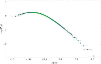
Figure 1: Comparison between numerical (points with ranges) and analytic results (starred points) for the distribution of integrated column depths.

We now discuss the distribution of magnifications due to a single halo. The halo has two distinct regions, the core $x<R_{s}$ and the external region $R_{s}<x<CR_{s}$. Here $x$ is the physical distance. To compute the magnification, we first compute the lensing convergence, $\kappa$, analytically. For a general density contrast $\delta\left(\mathbf{s}\right)=\Delta\rho\left(\mathbf{s}\right)/\rho_{\mathrm{FRW}}$ this is given by

$$\kappa=\frac{3}{2}\frac{H_{0}^{2}}{c^{2}}\Omega_{{\rm M}}\int_{0}^{y_{S}}dy\frac{y\left(y_{S}-y\right)}{y_{S}a_{{\rm ex}}\left(z\right)}\delta\left(y,\;z\right),$$ (10)

where $y$ is comoving distance along the ray, $y_{S}$ is the comoving distance to the source, $a_{{\rm ex}}\left(z\right)=\left(1+z\right)^{-1}$, $H_{0}$ is the Hubble constant, $c$ is the velocity of light, $\Omega_{{\rm M}}$ is the matter fraction and $z=z\left(y\right)$ is redshift. Combining the halo profile (1) and the second term in Eq. (4) with Eq. (10) gives for the lensing convergence due to the halo

$$\kappa\left(b\right)=\frac{8\pi Ga_{{\rm ex}}\left(z\right)}{c^{2}}(\rho_{0}R_{s})\frac{y\left(y_{{\rm S}}-y\right)}{y_{{\rm S}}}$$

$$\left[\kappa_{{\rm core}}\Theta\left(R_{s}-b\right)+\kappa_{{\rm out}}\Theta\left(b-R_{s}\right)\Theta\left(CR_{s}-b\right)\right].$$ (11)

Here $b=\left|\mathbf{b}\right|$ is the physical impact parameter

$$\kappa_{{\rm core}}=\left(-\frac{\sqrt{C^{2}-\alpha}}{\left(1-\alpha\right)\left(1+C\right)}+\frac{2}{\left(1-\alpha\right)^{3/2}}\right.$$

$$\left.\left[\tanh^{-1}\left(\frac{\sqrt{1-\sqrt{\alpha}}}{\sqrt{1+\sqrt{\alpha}}}\right)-\tanh^{-1}\left(\frac{\sqrt{1-\alpha}}{C+\sqrt{C^{2}-\alpha}+1}\right)\right]\right)$$ (12)

and

$$\kappa_{{\rm out}}=\left(\frac{\sqrt{C^{2}-\alpha}}{\left(\alpha-1\right)\left(1+C\right)}-\right.\frac{2}{\left(\alpha-1\right)^{3/2}}$$

$$\left.\left[\tan^{-1}\left(\frac{\sqrt{\sqrt{\alpha}-1}}{\sqrt{\sqrt{\alpha}+1}}\right)-\tan^{-1}\left(\frac{\sqrt{\alpha-1}}{C+\sqrt{C^{2}-\alpha}+1}\right)\right]\right).$$ (13)

Here $\Theta$ is the step function and $\alpha=b^{2}/R_{{\rm s}}^{2}$. Note that $\alpha<1$ for $b<R_{{\rm s}}$, $\alpha>1$ for $R_{{\rm s}}<b<CR_{{\rm s}}$ and $\kappa=0$ for $b>CR_{{\rm s}}$.

Finally, the mean of the lensing convergence for a single halo is obtained by averaging over the impact parameter

$$\hat{\kappa}=\frac{2}{\left(CR_{{\rm s}}\right)^{2}}\int_{0}^{CR_{{\rm s}}}\kappa\left(b\right)bdb$$ (14)

$$\;\;\;\;\;\;\;\;\;\;\;\;\;\;\;\;\;\;\;\;\;\hat{\kappa}=\frac{8\pi Ga_{{\rm ex}}\left(z\right)}{c^{2}}(\rho_{0}R_{s})\frac{y\left(y_{{\rm S}}-y\right)}{y_{{\rm S}}}\frac{M_{{\rm halo}}}{\left(CR_{{\rm s}}\right)^{2}}.$$ (15)

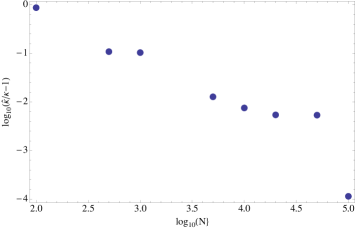
Figure 2: The difference between numerically $\left(\kappa\right)$ and analytically computed mean convergences $\left(\hat{\kappa}\right)$ as a function of number of runs $N$, for one void, comoving void radius $R$ = 35 Mpc, and fraction of void mass on the shell today $0.9$. Our numerical simulations agree with the analytic result to $<1\%$ for $N=10^{4}$.

We define $\eta=\int\rho\left(z\right)dz$ to be the integrated column density which is proportional to the convergence $\kappa$. Figure 1 is a comparison of $\log_{10}\left(P\left(\eta\right)\right)$, the logarithm of the probability distribution of $\eta$, computed analytically (starred points, Eq. (APPENDIX A: COLUMN DEPTH) from Appendix A) and the results from our code (points associated with the $\eta$ bins). Within each $\eta$ bin, the mean of the bins agree well with analytic results. The width of the bins represents the sampling accuracy within those bins, the centers of halos are sampled less than the rest of the halos.

To further assess the accuracy of our numerical results, we compute the mean of the distribution for a single halo for different numbers of runs ($N$), and compare this with the analytic expression (15). We find that the results from our numerics agree with the theoretical prediction with an accuracy $\sim N^{-1/2}$ as expected. In Figure 2, we plot the estimator of the mean as a function of $N$. We see that the accuracy is <1% for $N=10^{4}$. For the rest of the simulations in this paper, we will use $N=10^{4}$.

IV Results for the Swiss Raisin Nougat Model

The Swiss Raisin Nougat (SRN) model is an idealized Swiss Cheese model containing spherical voids with comoving radius $Y_{{\rm void}}=35$ Mpc. As explained earlier, the matter in the interior moves towards the outer edges of the void with the evolution of the Universe. For a particular void at some redshift, we break up the mass on the shell of the void into halos with NFW profiles and randomly distribute them on the shell. The mass in the interior is smeared smoothly inside the sphere with a uniform mass density. The parameters of this model are listed in Table II.

A key change from our void models in p3Ref1 is that there is no longer a zero thickness shell. One of the issues encountered in that model was the logarithmic divergence in the variance of the lensing convergence distribution due to the zero thickness assumption. Here, however, we break up the void surface into halos and the effective thickness of the shell is set by the size of these halos which acts as a natural cutoff. Hence, the divergence is avoided which makes for a more realistic and robust model.

Quantity	Value
$\Omega_{{\rm M}}$	0.3
$\Omega_{\Lambda}$	0.7
$H_{0}$	70 $\mathrm{kms^{-1}Mpc^{-1}}$
$Y_{{\rm void}}$	$35$ Mpc
Halo profile	NFW
Present fraction of void mass on shell	0.9
Fraction of shell mass in halos	1.0
Fraction of interior mass in halos	0.0

Table 2: Parameters of SRN model

IV.1 Probability of intersecting a halo

The expected number of times a light ray hits a halo is given by the ratio of the total projected area of all the halos in a void to the projected area of the void. The expected number of intersections at comoving impact parameter $p=\left|\mathbf{p}\right|$ (comoving distance from the center of the void) through the shell at redshift $z$ is

$$N_{{\rm int}}\left(p,\>z\right)=\frac{f\left(z\right)M_{{\rm void}}\left(z\right)}{4\pi Y_{{\rm void}}^{2}a_{{\rm ex}}^{3}\left(z\right)M_{{\rm halo}}}\pi R_{{\rm halo}}^{2}a_{{\rm ex}}^{3}\left(z\right)\times$$

$$\int_{0}^{\sqrt{Y_{{\rm void}}^{2}-p^{2}}}ds\delta\left(\sqrt{s^{2}+p^{2}}-Y_{{\rm void}}\right)$$ (16)

$$=\frac{f\left(z\right)M_{{\rm void}}\left(z\right)R_{{\rm halo}}^{2}}{2Y_{{\rm void}}\sqrt{Y_{{\rm void}}^{2}-p^{2}}a_{{\rm ex}}^{2}\left(z\right)M_{{\rm halo}}}.$$ (17)

Here $s$ is the comoving distance from the center of a void and $R_{{\rm halo}}=CR_{{\rm s}}$ is the physical radius of the halo. Averaging over the impact parameter, $p$, gives

$$N_{{\rm int}}\left(z\right)=\frac{f\left(z\right)M_{{\rm void}}\left(z\right)R_{{\rm halo}}^{2}}{Y_{{\rm void}}^{2}a_{{\rm ex}}^{2}\left(z\right)M_{{\rm halo}}}.$$ (18)

Note that the void radius $Y_{{\rm void}}$ is comoving while the halo radius $R_{{\rm halo}}$ is physical. Both these parameters are fixed and do not evolve with time. For example, for a void placed at redshift 0, $N_{{\rm shell}}\left(0\right)\simeq 0.4$.

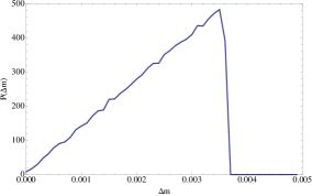
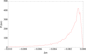
Figure 3: The probability distribution of magnitude shifts $\Delta m$ for a simulation in the SRN model with $\Omega_{M}=0.3$, with one void of radius 35 Mpc at $z=0.45$ and sources placed at $z_{s}=1$, and fraction of void mass on the shell today $f=0.9$. Top: The probability distribution of magnitude shifts $\Delta m$ for a single void for $\Delta m$ positive. Bottom: The probability distribution for magnitude shifts $\Delta m$ for a single void for $\Delta m$ negative. The total probability for $\Delta m<0$ is $\simeq 0.8.$

IV.2 One void

In this section we will focus on a single void at redshift 0.45 and a source at redshift 1. We calculate the expected number of halo intersections for a light ray from Eq. (18). For a 35 Mpc void, using the halo parameters from Section II, we get $N_{{\rm shell}}\left(0.45\right)\simeq 0.8$. For $N=10^{4}$ runs, we keep track of the number of times that light rays hit halos and we obtain 8064 instances, which agrees well with our prediction. We use the density perturbation (4) for the SRN model and compute the lensing convergence $\kappa$ by summing the result (11) over all intersected halos.

For the rest of the paper, we will concentrate on the distribution of the magnitude shift $\Delta m$, which is a function of lensing convergence $\kappa$

$$\Delta m=\frac{2.5}{\ln 10}\ln\left|\left(1-\kappa\right)^{2}-\gamma^{2}\right|.$$ (19)

Here $\gamma$ is the shear, which we will discuss in the next section. Figure 3 shows the probability distribution $P\left(\Delta m\right)$ of magnitude shifts $\Delta m$ we obtain for a single void placed at $z=0.45$ (without shear).

A notable feature of this distribution is that it is bimodal, with peaks at both positive and negative $\Delta m$ (We plot separately the distribution for positive $\Delta m$ and for negative $\Delta m$, since the relevant scales for these two regions of the probability distribution are very different). The peak at positive $\Delta m$ is predominantly due to rays that do not intersect any halos, and are demagnified by their passage through the underdense void interior. The peak at negative $\Delta m$ is predominantly due to rays which intersect one or more halos and are consequently magnified.

We can also compute the mean of each of these distributions and compare them with analytical expressions. The means for $\Delta m>0$, $\left\langle\Delta m\right\rangle_{+}$ and for $\Delta m<0$, $\left\langle\Delta m\right\rangle_{-}$ are defined to be

$$\left\langle\Delta m\right\rangle_{+}=\int_{0}^{\infty}\Delta mP\left(\Delta m\right)d\left(\Delta m\right),$$ (20)

$$\left\langle\Delta m\right\rangle_{-}=\int_{-\infty}^{0}\Delta mP\left(\Delta m\right)d\left(\Delta m\right).$$ (21)

We decompose the full distribution of magnification as a sum

$$P\left(\Delta m\right)=\sum_{n=0}^{\infty}\mathcal{P}_{n}P_{n}\left(\Delta m\right),$$ (22)

where $\mathcal{P}_{n}$ is the probability of $n$ halo intersections and $P_{n}\left(\Delta m\right)d\left(\Delta m\right)$ is the probability of having a magnitude shift between $\Delta m$ and $\Delta m+d\left(\Delta m\right)$ given that there are $n$ intersections.

The analytic expression for the magnitude shift for zero halo intersections is p3Ref1

$$\Delta m=2.5\log_{10}\left|\left(1-\kappa_{{\rm interior}}\right)^{2}\right|,$$ (23)

where

$$\kappa_{{\rm interior}}\left(p\right)=-3\frac{H_{0}^{2}}{c^{2}}\Omega_{{\rm M}}f\left(z\right)\frac{y\left(y_{S}-y\right)}{y_{{\rm S}}a_{{\rm ex}}\left(z\right)}\sqrt{Y_{{\rm void}}^{2}-p^{2}}.$$ (24)

Here $f\left(z\right)$ is the fraction of the mass of the void on the shell, $y$ is the comoving distance to the void, $y_{S}$ is comoving distance to the source, $a_{ex}\left(z\right)$ is the scale factor and $p$ is the comoving impact parameter. Note that for this one void case, essentially all the negative $\Delta m$ contributions are due to intersections with one halo and the positive $\Delta m$ contributions are due to the void interior (i.e., no halo intersections). In this approximation, Eqs. (20) and (21) reduce to

$$\left\langle\Delta m\right\rangle_{+}\simeq\mathcal{P}_{0}\int_{-\infty}^{\infty}\Delta mP_{0}\left(\Delta m\right)d\left(\Delta m\right)$$ (25)

and

$$\left\langle\Delta m\right\rangle_{-}\simeq\mathcal{P}_{1}\int_{-\infty}^{\infty}\Delta mP_{1}\left(\Delta m\right)d\left(\Delta m\right).$$ (26)

We can compute $\mathcal{P}_{0}$ and $\mathcal{P}_{1}$ from Eq. (18) assuming $\mathcal{P}_{0}+\mathcal{P}_{1}=1$ for the one void case, obtaining $\mathcal{P}_{1}=0.8$ and $\mathcal{P}_{0}=0.2$ which matches with our simulations. The numerically computed means (4.5) and (4.6) of the magnified and demagnified distributions agrees with their corresponding halo and void interior theoretical values [computed from Eqs. (12) - (13), (19) & (24)] to $\sim 0.5\%$. We also numerically compute the mean lensing convergence obtaining $-5\times 10^{-4}$ magnitudes with standard deviation $2\times 10^{-3}$ magnitudes. Thus the mean is consistent with zero as we would expect from a general theorem.

IV.3 Shear

So far in our analysis we have not included shear. We can include it as follows. The matrix $L_{\;C}^{A}$ for the $j$-th void defined in Eq. (2.15c) of p3Ref1 is

$$L_{AB}=-2\int dy\left[\nabla_{A}\nabla_{B}\delta\Phi+{1\over 2}\left(\delta\Phi\right)_{,yy}\delta_{AB}\right].$$ (27)

where $\delta\Phi$ is the potential perturbation, $y$ is comoving distance, the derivatives are with respect to comoving coordinates, and the integral is taken over just the $j$-th void. We decompose $L_{AC}$ into a trace part and a trace free part to obtain

$$L_{AB}=\frac{1}{w_{j}}\left[\kappa_{j}\delta_{AB}+\gamma_{jAB}\right],$$ (28)

where $w_{j}=y_{j}\left(y_{S}-y_{j}\right)/y_{S}$, $y_{j}$ is the comoving distance to the $j$-th void, $\kappa_{j}$ is the lensing convergence we computed previously [Eqs. (11) - (13) and (24)], and the matrix $\boldsymbol{\gamma}_{j}$ is traceless. We compute the potential perturbation from the density perturbations (3) and (4), and insert into Eqs. (27) and (28) to obtain the shear term $\gamma_{jAB}$ which will be of the form $\gamma_{j}\epsilon_{AB}$ on a suitable choice of basis. For a single NFW halo the potential perturbation is

$$\delta\Phi\left(r\right)=-4\pi G\rho_{0}R_{s}^{2}\left[\frac{R_{s}}{r}\ln\left(1+\frac{r}{R_{s}}\right)-\frac{1}{1+C}\right].$$ (29)

The shear due to the void interior and the halos on the shell is

$$\gamma_{\;B}^{A}=\left(\gamma_{{\rm void}}\right)_{\;B}^{A}+\sum_{i=1}^{N_{\rm{shell}}}\left(\gamma_{{\rm halo}}^{i}\right)_{\;B}^{A},$$ (30)

where

$$\left(\gamma_{{\rm void}}\right)_{\;B}^{A}=3\frac{H_{0}^{2}}{c^{2}}\Omega_{{\rm M}}f\left(z\right)\frac{y\left(y_{S}-y\right)}{y_{{\rm S}}a_{{\rm ex}}\left(z\right)}\frac{Y_{{\rm void}}}{\beta}\left(\delta_{B}^{A}-2\hat{p}^{A}\hat{p}_{B}\right)$$

$$\left(\frac{2}{3}-\Theta\left(Y_{{\rm void}}-p\right)\left[\frac{2}{3}\left(1-\beta\right)^{3/2}+\beta\left(1-\beta\right)^{1/2}\right]\right),$$ (31)

and

$$\left(\gamma_{{\rm halo}}^{i}\right)_{\;B}^{A}=\frac{\delta_{B}^{A}-2\hat{b}_{i}^{A}\hat{b}_{Bi}}{b_{i}^{2}}\Biggl{[}-4M_{{\rm halo}}$$

$$\left.+16\pi\int_{b_{i}}^{CR_{s}}drr\rho_{{\rm halo}}\left(r\right)\sqrt{r^{2}-b_{i}^{2}}+8\pi\int_{b_{i}}^{CR_{s}}drr\frac{\rho_{{\rm halo}}\left(r\right)}{\sqrt{r^{2}-b_{i}^{2}}}\right].$$ (32)

Here $\mathbf{p}=p\hat{p}^{A}\mathbf{e_{A}}$ is again the comoving impact parameter to the void, $\beta=p^{2}/Y_{{\rm void}}^{2}$ and $\mathbf{b}_{i}=b_{i}\hat{b}_{i}^{A}\mathbf{e_{A}}$ is the physical impact parameter of the light ray to the $i$-th halo. The first term in Eq. (32) is the point mass contribution of the halos. The second and third terms in Eq. (32) are non zero only for intersected halos. Evaluating the integrals using the NFW profile (1), we find that the intersected halo contribution $\left(\gamma_{{\rm int}}^{i}\right)_{\;B}^{A}$ is

$$\left(\gamma_{{\rm int}}^{i}\right)_{\;B}^{A}=\frac{16\pi G}{c^{2}}a_{{\rm ex}}\left(z\right)\rho_{0}R_{s}\frac{y\left(y_{S}-y\right)}{y_{S}}\left(\delta_{B}^{A}-2\hat{b}_{i}^{A}\hat{b}_{Bi}\right)\gamma_{h}.$$ (33)

Here for $\alpha<1$

$$\gamma_{h}=\frac{1}{\alpha}\left\{\frac{\left(2-\alpha\right)\sqrt{C^{2}-\alpha}}{2\left(\alpha-1\right)\left(C+1\right)}+\ln\left[\frac{C+\sqrt{C^{2}-\alpha}}{\sqrt{\alpha}}\right]\right.$$

$$+\frac{\left(3\alpha-2\right)}{\left(1-\alpha\right)^{3/2}}\left(\tanh^{-1}\left[\sqrt{\frac{1-\sqrt{\alpha}}{\sqrt{\alpha}+1}}\right]\right.$$

$$\left.\left.-\tanh^{-1}\left[\frac{\sqrt{1-\alpha}}{C+1+\sqrt{C^{2}-\alpha}}\right]\right)\right\},$$ (34)

and for $1<\alpha<C^{2}$

$$\gamma_{h}=\frac{1}{\alpha}\left\{\frac{\left(2-\alpha\right)\sqrt{C^{2}-\alpha}}{2\left(\alpha-1\right)\left(C+1\right)}+\ln\left[\frac{C+\sqrt{C^{2}-\alpha}}{\sqrt{\alpha}}\right]\right.$$

$$-\frac{\left(3\alpha-2\right)}{\left(\alpha-1\right)^{3/2}}\left(\tan^{-1}\left[\sqrt{\frac{\sqrt{\alpha}-1}{\sqrt{\alpha}+1}}\right]\right.$$

$$\left.\left.-\tan^{-1}\left[\frac{\sqrt{\alpha-1}}{C+1+\sqrt{C^{2}-\alpha}}\right]\right)\right\},$$ (35)

where $\alpha=b_{i}^{2}/R_{s}^{2}$.

From Eqs. (33) - (35), $\gamma^{2}\sim 1/b^{4}$. Therefore contributions from shear are heavily suppressed. In our numerical analysis, the standard deviation changes by less than $3\%$ if shear is neglected.

IV.4 Qualitative features of magnification distributions

With the accuracy of our method tested, we now explore the magnification distributions in more general situations with many voids, distributed along the line of sight with random impact parameters according to the algorithm discussed in p3Ref1 . For example, for sources at redshift $z_{{\rm s}}=1$, there are 47 voids of comoving radius $Y_{{\rm void}}=35$ Mpc along the line of sight. We follow steps 1 to 8 of Section IIC of our previous paper p3Ref1 , but with the modification that the matrices $\mathbf{J}$, $\mathbf{K}$, $\mathbf{L}$ and $\mathbf{M}$ now incorporate the effects of the halo substructure of the shell.

In Figure 4, we plot the log of the magnification distribution for $z_{s}=0.5,\>1.0\>$ and $1.5$. In our SRN model, we have voids with randomly distributed halos on their surface and a smooth interior. We denote by $\mathcal{P}_{n}$ the probability of having $n$ halo intersections. The whole probability distribution can be decomposed into a sum of probability distribution for different numbers of halo intersections, like in Eq. (22). We plot the 25%, 50% and 75% quartiles of the distributions as horizontal lines (top, middle and bottom respectively). For high redshifts, most of the probability is concentrated in the demagnified areas where the rays hit only a few halos or simply pass through without hitting any.

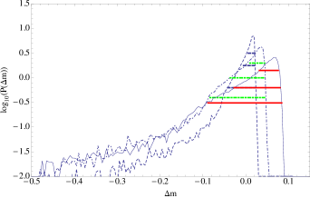
Figure 4: The probability distributions of magnitude shifts $\Delta m$ for the SRN model with sources at redshifts of $z_{s}=0.5$ (dashed), $z_{s}=1.0$ (dot-dashed) and $z_{s}=1.5$ (solid), for comoving voids of radius R = 35 Mpc with 90% of the void mass on the shell today. The horizontal lines are the 25% (top), 50% (middle) and 75% (bottom) quartiles about the peak of the distribution.

Note that the total probability in the tail on the magnification side $\left(\Delta m<0\right)$ increases with redshift, because of the increased probability of hitting halos at higher redshifts. For example, at $\Delta m=-0.2$, we would expect the probability density for $z_{{\rm s}}=1.5$ to be roughly 2-3 times as large as the probability density for $z_{{\rm s}}=0.5$ because the number of voids that rays have to pass through in the former case is 62 where as for the latter it is 27. In addition, rays at high redshifts have more close encounters with halos that generate shear.

Figure 5 shows the standard deviation of the distribution, $\sigma_{m}$, as a function of redshift of the source, $z_{{\rm s}}$. This standard deviation for voids and halos is $\sim 3$ times larger at $z_{{\rm s}}=1$ than that for a model with mass compensated voids with a shell thickness of 1 Mpc and no halos [1]. We note that most of the contribution to the standard deviation come from rays that intersect halos. Also, the standard deviation we compute agrees well with that computed using other methods. For example, our standard deviation for $z_{{\rm s}}=1.5$ is $\sigma_{m}=0.072$, which agrees to within 20% with the standard deviation of the distribution shown in Figure 1 of Ref. p3Ref5 . We compare our results to those obtained using another method introduced in Refs. p3Ref11 ; p3Ref12 in the next subsection.

In Appendix B we derive the following approximate result for the standard deviation:

$$\sigma_{m}={5\over{\log\left(10\right)}}\left({\Omega_{M}\over 2}{\overline{g}_{h}}\sum_{j}{(H_{0}Y_{\rm{void}}f_{j})H_{0}^{2}w_{j}^{2}}\right.$$

$$\;\;\;\;\;\;\;\;\;\;\;\;\;\;\;\;+\left.{\Omega_{M}^{2}\over 2}\sum_{j}{(H_{0}Y_{\rm{void}}f_{j})^{2}H_{0}^{2}w_{j}^{2}\over a_{j}^{2}}\right)^{1\over 2}.$$

Here ${\overline{g}_{h}}$ is a dimensionless parameter which represents the contribution from halos whose detailed form is given by Eq. (B21), $Y_{\rm{void}}$ is the comoving radius of the voids, $f_{j}=f\left(z_{j}\right)$ is the fraction of the mass of $j$-th void on its surface and $a_{j}=a\left(z_{j}\right)$ is the scale factor. The result (4.21) assumes statistical independence of halos within voids and also of voids from one another and neglects lensing shear. There are two main qualitative features of the result (4.21). First, the contribution to the standard deviation due to the halos [the first term in Eq. (4.21)] depends primarily on their gravitational potential, and the contribution due to voids [the second term in Eq. (4.21)] depends primarily on the size of the underdense core. Second, the halo contribution is bigger than the interior contribution and hence the standard deviation is dominated by halos. For example, using the above expression, the ratio of the contribution due to the halos to the contribution due to the core is $\sim 100$ for $z_{s}=1$ and for the void and halo parameters defined in Table II.

We discuss further the analytic calculation of standard deviation without shear in Appendix B. Our numerical results agree with these approximate analytic predictions to within $\sim 20\%$.

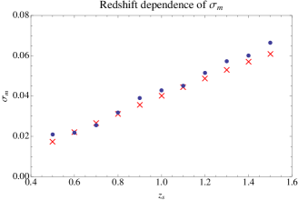
Figure 5: Redshift dependence of standard deviation of distribution of magnitude shifts, for comoving voids of radius R = 35 Mpc with 90% of the void mass on the shell today. The crosses are analytic results.

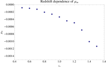
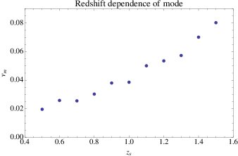
Figure 6: Plot of mean (top) and mode (bottom) of the distribution as a function of redshift in SRN. The mode takes on increasingly positive values with redshift and the mean is increasingly negative with redshift.

IV.5 Redshift dependence of mean and mode of magnitude shift

While the mean of lensing convergence vanishes, the mean magnitude shift does not, because magnitude shift is a nonlinear function of $\kappa$, defined in Eq. (19). Figure 6a shows the mean $\mu_{m}$ of the distribution of magnification shifts $\Delta m$, which increases with redshift as $\propto\sigma_{m}^{2}$. This is the expected theoretical behavior: for small values of $\kappa$ and ignoring shear, we can approximate Eq. (19) as

$$\Delta m\simeq\frac{5}{\ln 10}\ln\left|\left(1-\kappa\right)\right|\simeq\frac{5}{\ln 10}\left(-\kappa-\frac{1}{2}\kappa^{2}\right).$$ (35)

The mean magnitude shift is then proportional to the mean of the square of $\kappa$ as the mean of $\kappa$ is vanishing,

$$\mu_{m}\simeq-\frac{2.5}{\ln 10}\left\langle\kappa^{2}\right\rangle.$$ (36)

The standard deviation, from Eq. (13) in p3Ref1 simplifies to

$$\sigma_{m}=\frac{5}{\ln 10}\sqrt{\left\langle\kappa^{2}\right\rangle},$$ (37)

and so $\mu_{m}\simeq-0.23\sigma_{m}^{2}$ which agrees with our numerical results to within $\sim 10\%$.

On average there is a small overall magnification of light beams. Figure 6b shows the mode $\nu_{m}$, the location of the maximum of the PDF, which also increases with redshift. The modes of the magnification to redshift 1.5 are positive because an overall demagnification occurs for most of the light rays as they pass through the interior of the voids while hitting halos. Note that the modes are larger than the corresponding means.

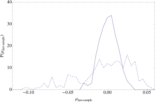
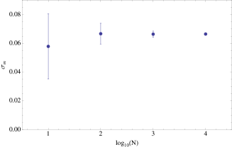
Figure 7: Top: Plot of distribution of means of 200 samples of 10 (dashed) and 100 (solid) sources each at redshift $z_{s}=1.5$. The mean of the distribution of means is 0.011 magnitudes and the standard deviation is 0.028 magnitudes for the sample of 10. The respective numbers for the sample of 100 sources is 0.0004 and 0.011, showing that more sources reduces demagnification bias. Bottom: Plot of the range of standard deviation for samples of different sizes showing convergence as $N\to 10^{4}$.

In realistic surveys, one can expect to find only a few standard candle sources for every redshift or every redshift bin. This severely constrains the accuracy of the cosmological parameters we can infer from such observations. To illustrate the extent of lensing degradation in measuring cosmological parameters, we pick 200 sets of randomly placed 10 or 100 sources at $z_{s}=1.5$. We find the mean of each of these samples in the set and plot the resulting distribution of means in Figure 7 (top). The mean of the means for the 10 sources case is 0.011 magnitudes and the standard deviation of the means is 0.028 magnitudes. The respective numbers for the 100 sources case are 0.0004 and 0.011 magnitudes. A change in cosmological parameters by $1\%$ implies a change in $\Delta m$ of 0.015 magnitudes. Thus for data acquired from surveys, the lensing degradation is quite a significant effect, although it can be mitigated by increasing the number of sources. This is also seen in Figure 7 (bottom) where we plot the range of standard deviation for samples of different sizes. For a large enough sample, the bias in magnification can be accurately taken into account. This effect is studied in p3Ref5 which shows that lensing degradation effectively decreases the number of useful supernovae by a factor of 3 at source redshift 1.5.

Our work is broadly consistent with other work, p3Ref11 ; p3Ref12 ; p3Ref14 ; p3Ref15 ; p3Ref16 ; p3Ref17 ; p3Ref18 ; p3Ref19 ; p3Ref20 ; p3Ref21 ; p3Ref22 in this area. A similar computational method has been developed by Kainulainen & Marra, Refs. p3Ref11 ; p3Ref12 . Their model consists of filaments and halos of various sizes, where the mass fraction in filaments is 0.5 and the rest is distributed in halos. To compare with their results, we use the SRN model and choose parameters to match their cosmology, i.e., $\Omega_{{\rm M}}=0.25$, $z_{s}=1.5$, $H_{0}=73$ $\mathrm{kms^{-1}Mpc^{-1}}$ and $f=0.5$. We do not include shear for this comparison as it is neglected in their analysis. Our magnification PDF qualitatively agrees with that of Kainulainen & Marra as shown in Figure 8.

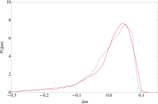
Figure 8: The probability distributions of magnitude shifts $\Delta m$ for an SRN model (dashed lines) with sources at redshift $z_{s}=1.5$, comoving voids of radius 35 Mpc, with 50% of the void mass in halos today, $\Omega_{{\rm M}}=0.25$, $\Omega_{\Lambda}=0.75$, $H_{0}=73$ $\mathrm{kms^{-1}Mpc^{-1}}$ and with no shear, compared to the results in Figure 5 (we reproduced the plot by picking points from their figure) of the model in Kainulainen and Marra p3Ref12 where they have 50% of mass in halos and all other parameters same as ours. The two distributions are qualitatively similar.

V Results for Swiss Raisin Raisin model

In our Swiss Raisin Raisin (SRR) model, in addition to replacing the smooth surface density on the shell with a collection of halos, the mass in the interior is also broken up into NFW halos with the same parameters as before. The parameters of the SRR model are listed in Table III.

Quantity	Value
$\Omega_{{\rm M}}$	0.3
$\Omega_{\Lambda}$	0.7
$H_{0}$	70 $\mathrm{kms^{-1}Mpc^{-1}}$
$Y_{{\rm void}}$	$35$ Mpc
Halo profile	NFW
Present fraction of void mass on shell	0.9
Fraction of shell mass in halos	1.0
Fraction of interior mass in halos	1.0

Table 3: Parameters of SRR model

V.1 A single void

In this section we focus on a single void with no shear. Again, we use Eqs. (4), (12) - (13) and (23) to compute the magnifications. For a 35 Mpc void and using the same halo parameters as in Section II, the intersection probability remains about the same as in the previous model. The change due to the addition of a few halos in the vast interior region is negligible. The expected number of halo intersections $N_{\rm int}\left(z\right)$ is given by Eq. (18) with the shell mass replaced by the total void mass $M_{\rm void}$

$$N_{\rm int}\left(z\right)=\frac{M_{\rm void}R_{{\rm halo}}^{2}}{Y_{{\rm void}}^{2}a_{{\rm ex}}^{2}\left(z\right)M_{{\rm halo}}}$$ (38)

Using the same parameters as in the one void case in the SRN model we obtain $N_{\rm int}\left(0.45\right)\simeq 0.88$. We find that light rays hit halos 8720 times for $N=10^{4}$ runs which translates to an intersection probability of $\sim 88\%$ and agrees well with Eq. (38).

Again we find a bimodal distribution of magnitude shifts. In Figure 9, this bimodal distribution is superimposed on the SRN plots from Figure 3. Since the density contrast in the interior is increased by $\sim 10\%$ (if halos are not hit) compared to our SRN model, the demagnified distribution shifts towards the right. Figure 9a shows this shift in underdense part of the distribution. Figure 9b is the $\Delta m<0$ part of the distribution. This accounts for roughly 88% of the total distribution and it is similar to the distribution in Figure 3b.

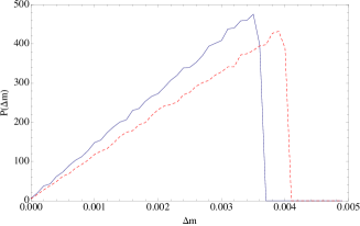
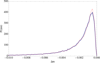
Figure 9: The probability distribution of magnitude shifts $\Delta m$ for a simulation in the SRR model (dashed line) superimposed on the corresponding probability distribution in the SRN model (solid line) with $\Omega_{M}=0.3$, with one void of radius 35 Mpc and fraction of void mass on the shell today $f=0.9$. Note that the demagnified part, (top), is shifted because there is an increase in the density contrast in the interior of voids, while the magnified part, (bottom), is mostly unchanged.

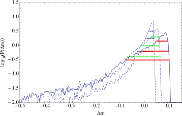
Figure 10: The probability distributions of magnitude shifts $\Delta m$ for the SRR model with sources at redshifts of $z=0.5$ (dashed), $z=1.0$ (dot dashed) and $z=1.5$ (solid), for voids of comoving radius R = 35 Mpc, with 90% of the void mass on the shell today. We see the same qualitative features as in SRN for the corresponding redshift but all the distributions are shifted towards demagnification. The horizontal lines are the 25% (top), 50% (middle) and 75% (bottom) quartiles of the distribution from the peaks.

V.2 Redshift dependence of distributions

Next we explore the bias (i.e., the mean of the distribution) due to halos and voids for sources at various redshifts, namely, for $z_{{\rm s}}=0.5,\>1.0\>$ and $1.5$. To compute the shear in this case, for the void contribution we use Eq. (24) but with $f\left(z\right)=1$, and in Eqs. (33) - (35), we sum over both the surface and interior halos. The magnifications shown in Figure 10 are predominantly due to halos while the mostly empty interior has a demagnifying effect. Due to the increased underdensity inside the void, the magnitudes shift towards demagnification. The standard deviation for $z_{s}=1.5$ is $\sigma_{m}=0.072$. Again we note that the modes are larger than the means and also shift towards the demagnification end of the plot with increasing redshift. The tails of these distributions are similar to the ones obtained in the SRN model in Figure 4.

Next we consider the mean magnitude shift, $\mu_{m}$, and its mode, $\nu_{m}$, in the two models. The key feature here is that the underdense interior is more prominent in the SRR model. We expect that the mean magnitude shift and its mode should shift and the difference in the means should increase with redshift. In Figure 11, we plot the means and modes for the two models and we show that $\mu_{m}$ for SRR is $\sim 10-20\%$ greater than that for SRN at $z_{{\rm s}}=1$.

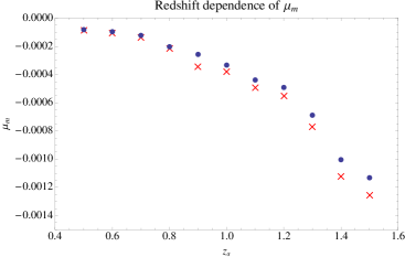
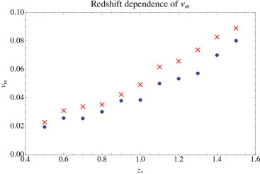
Figure 11: The mean and mode of magnification shift for the two models - Points: SRN; Crossed points: SRR. Top: The mean of magnification shift, $\mu_{m}$, for the two models. We see that the difference in the means increases with redshift and at $z=1$ and it is $\sim 10\%$. Bottom: The mode of magnification shift, $\nu_{m}$, for the two models. We see that the difference in the means increases with redshift and at $z=1$ and it is $\sim 20\%$.

These two models are interesting because they represent the two possible extremes of the matter distribution in voids - one where the matter is smoothly distributed with no structure and another with only chunky NFW halos. In reality, the underdense region will be composed of both halos and an ambient intergalactic medium. By studying the completely smooth interior case (SRN) and the completely granular interior case (SRR), we expect to bracket the true distribution.

V.3 Effect of large scale structure

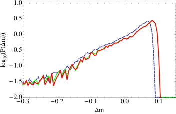
Figure 12: The probability distributions of magnitude shifts $\Delta m$ for simulations in SRR (solid), the SRN model (dot dashed), for comoving voids of radius R = 35 Mpc with $f=0.9$ today. Also shown is the model with uniformly distributed halos everywhere and with no voids (dashed - this is the $f=0$ limit of the SRR model) with source at redshifts of $z=1.5$. The distributions are similar in the SRR models because the expected number of halos intersected is independent of of the radial distribution of halos, where as the distribution in the SRN model is qualitatively similar but is shifted towards negative magnifications.

Previous studies in the literature have modeled the magnification effects of only voids p3Ref1 ; p3Ref7 ; p3Ref10 or only halos p3Ref3 ; p3Ref5 ; p3Ref11 , while other studies have considered very specific models with a particular distribution of filaments and halos p3Ref12 . In our work, we present two models that incorporate the effects of both halos and voids. We have considered cosmological models where at large scales matter evolves to cluster on the edges of spherical voids.

One limit of our model is the case where there are no halos on the surface and the interior is composed entirely of halos. This corresponds to the $f=0$ limit of the SRR model, a "no void limit". In Figure 12, we compare the magnification distribution we obtain for this configuration for $z_{s}=1.5$ to the corresponding distribution in the SRR and SRN models, for comoving voids of radius R = 35 Mpc with 90% of the void mass on the shell today. From Eq. (38), the expected number of halo intersections in the SRR model is independent of the radial distribution of the halos and hence the SRR and no void distributions should be similar, as observed. However, in the SRN model the number of halo intersections is lower due to the smaller number of halos. Hence the distribution is shifted towards negative magnification shifts.

VI Conclusions

In this paper, we presented two simple models to study the effects of both voids and halos on distance modulus shifts due to gravitational lensing. Our results may be useful for future surveys that gather data on luminosity distances to various astronomical sources to constrain properties of the source of cosmic acceleration. The core of our model is constructed by considering a $\Lambda$CDM Swiss cheese cosmology with mass compensated, randomly located voids, while our small scale halo structures are non-evolving and chosen to be all the same size and with an NFW matter profile.

We used an algorithm, described in p3Ref1 , to compute the probability distributions of distance modulus shifts. The mean dispersion of the magnitude shift due to gravitational lensing due to voids and halos is $\sim 3$ times larger than due to voids alone with a shell thickness, p3Ref1 ; the dispersion $\sigma_{m}$ due to 35 Mpc voids and halos for sources at $z_{{\rm s}}=1.5$ is $\sigma_{m}=0.065-0.072$ (depending on the model). The mean magnitude shift due to voids and halos is of order $\delta m=-0.0010$ to $-0.0013$ (depending on the model). These values of $\sigma_{m}$ imply that large scale structure must be accounted for in using luminosity distance determinations for estimating precise values of cosmological parameters, such as those characterizing the dark energy equation of state.

We studied the distribution of magnitude shifts for three different source redshifts in each of our models. The qualitative dependence on redshift is similar to that of the previous void-only models p3Ref1 . We find that the voids do not significantly change the variance but do significantly change the demagnification tail and the mode. The mode lies on the demagnification side and the variance is largely due to halo intersections. The scale of voids is unimportant and the only discernable effect in the mode is seen when the void interior is smoothly distributed matter. As a result, our models bracket the range of possibilities of magnifications.

Our simple and easily tunable model for void and galaxy halo lensing can be used as a starting point to study more complicated effects. For example, one can use various algorithms to generate realizations of distributions of non-overlapping spheres in three dimensional space. Given such a realization one could use the algorithm of this paper to study correlations between magnifications along rays with small angular separations, which would be relevant to future small beam surveys p3Ref23 . Finally, our model is in general agreement with other simplified lensing models in the literature that focus on lensing due to both halos and larger scale structures, p3Ref12 ; p3Ref14 ; p3Ref15 ; p3Ref16 ; p3Ref17 ; p3Ref18 ; p3Ref19 ; p3Ref20 ; p3Ref21 ; p3Ref22 .

Our results for $\sigma_{m}$ in the SRN void model are represented within about 20% by an analytic model presented in detail in Appendix B. This model ascribes the magnitude shift entirely to the fluctuations in light beam convergence that results from passage through underdense cores and overdense halos; thus it ignores the contribution from shear, which we have found to be relatively small empirically. The final result for $\sigma_{m}^{2}$ is a sum of these two contributions. [See Eqs. (B20) and (B22)]. Although our simulations assumed a single halo mass $M_{h}$, radius $R_{h}$ and concentration $C$, and a single void radius, the analytic model allows distributions for these key quantities. The contribution from halos is proportional to a suitably weighted mean of $M_{h}\Psi_{2}(C_{h})/R_{h}^{2}$, where $\Psi_{2}(C_{h})$ is defined in Eq. (B16) and is displayed in Fig. 13. The contribution from the underdense void cores is proportional to the mean void radius. Typically, the contribution to $\sigma_{m}^{2}$ from halos is much larger than the contribution from void cores so $\sigma_{m}^{2}$ is larger for more massive or more compact halos.

We have seen that the results of our simulations depend on whether the underdense core consists of smoothly distributed dark matter (SRN) or is itself clumped into halos (SRR). In the extreme case in which the underdense core is entirely made of halos, the results do not depend on the core density, and is equivalent to the SR model that consists of halos distributed randomly within a void.

Although the analytic model was only developed for the SRN model, it could also be applied to the SRR model with any prescription for the fraction of the mass of the underdense core that is clumped into halos. For example, in the extreme case of total clumping we can use the analytic models in Appendix B with the substitution $f=1$ for all $z$ in all expressions derived there. For intermediate cases, a prescription for the fraction of the underdense core that remains smooth rather than clumped would be needed.

APPENDIX A: COLUMN DEPTH

In this appendix, we describe how we calculate the column density encountered by rays passing through halos in the SRN model. In our model for the voids, we break up the bounding shell of mass into halos with mass $M_{{\rm halo}}$. As a light ray passes through one of these halos, the beam will acquire some integrated column depth, $\eta=\int\rho\left(z\right)dz$, where the random variable $\eta$ depends on the impact parameter of the beam with respect to the halo center, $\rho\left(z\right)$ is the density profile of the halo and $y$ is the physical coordinate. The maximum value is for a beam going right through the center, and diverges for our NFW profile 1.

We use an NFW profile 1, for the matter distribution in halos, and the column depth is

$$\eta\left(b\right)=(2\rho_{0}R_{{\rm s}}^{3})\int_{0}^{\sqrt{\left(CR_{{\rm s}}\right)^{2}-b^{2}}}\frac{dz}{\sqrt{z^{2}+b^{2}}\left(\sqrt{z^{2}+b^{2}}+R_{{\rm s}}\right)^{2}}$$ (A1)

where we have changed from radial (in Eq. (1)) to Cartesian coordinates. Here the physical impact parameter is $b$ and $C$ is the ratio of the radius of the halo to its core radius. This reduces to the sum of two contributions

$$\eta_{{\rm halo}}\left(b\right)=\eta_{{\rm core}}\Theta\left(R_{{\rm s}}-b\right)+\eta_{{\rm out}}\Theta\left(b-R_{{\rm s}}\right)\Theta\left(CR_{{\rm s}}-b\right)$$ (A2)

where the relationship between the column depth $\eta\left(b\right)$ and the corresponding lensing convergence, $\kappa\left(b\right)$, is, from Eq. (3.1),

$$\eta\left(b\right)=\left(\frac{4\pi Ga_{{\rm ex}}\left(z\right)}{c^{2}}\frac{y\left(y_{{\rm S}}-y\right)}{y_{{\rm S}}}\right)^{-1}\kappa\left(b\right).$$

The lensing convergences is listed in Eqs. (12) and (13). Again, the contribution from outside a radius of $CR_{{\rm s}}$ is zero. The mean column density of halos is defined as

$$\eta_{{\rm halo}}=\frac{M_{{\rm halo}}}{\pi\left(CR_{{\rm s}}\right)^{2}}.$$

For the halos, even more important that $\eta$ is $d\eta/d\alpha$, where $\alpha=b^{2}/R_{{\rm s}}^{2}$; this is because the probability distribution for $\alpha$ is $d\alpha/C^{2}$, and therefore the probability distribution for $\eta$ for a single halo is

$$P_{{\rm halo}}\left(\eta\right)=\frac{1}{C^{2}\left|d\eta_{{\rm halo}}/d\alpha\right|}.$$

This is the quantity plotted in Figure 1.

APPENDIX B: ANALYTIC ESTIMATE OF STANDARD DEVIATION

In this appendix, we derive analytic results for the standard deviation of magnifications. Consider the mean of the contribution to the convergence (3.1) from the underdense core of the $j$-th void, which we will denote by $\kappa_{c,j}$. We find

$$\kappa_{c,j}=-{3H_{0}^{2}\Omega_{M}\over 2}\times{f_{j}y_{j}(y_{S}-y_{j})\over a_{j}y_{S}}\times 2\sqrt{Y_{j}^{2}-p_{j}^{2}}$$

where $Y_{j}$ is the comoving radius of the void, $a_{j}$ is the scale factor and $f_{j}$ is the fraction of the total void mass on the surface at redshift $z_{j}$. After averaging over impact paramters we obtain

$$\langle\kappa_{c,j}\rangle=-2\Omega_{M}H_{0}Y_{j}{f_{j}H_{0}y_{j}(y_{S}-y_{j})\over a_{j}y_{S}},$$

and therefore the net expected convergence from voids is

$$\langle\kappa_{c}\rangle=\sum_{j}\langle\kappa_{c,j}\rangle=-2\Omega_{M}H_{0}\sum_{j}{f_{j}Y_{j}H_{0}y_{j}(y_{S}-y_{j})\over a_{j}y_{S}}\leavevmode\nobreak\ .$$

Assuming a typical radius $Y_{j}\sim Y_{\rm{void}}$, there are about $(H_{0}Y_{\rm{void}})^{-1}$ terms in the sum, and consequently the overall average is $\sim\Omega_{M}$. In the limit that there are many voids along a given line of sight, we can replace the sum by an integral. The number of voids per interval $dy$ of comoving distance is $dy/2R$, and therefore if we define $\xi=H_{0}y$ we find

$$\langle\kappa_{c}\rangle=-2\Omega_{M}H_{0}\sum_{j}{f_{j}R_{i}H_{0}y_{j}(y_{S}-y_{j})\over a_{j}y_{S}}$$

$$\to-\Omega_{M}\int_{0}^{\xi_{S}}{d\xi f(\xi)\xi(\xi_{S}-\xi)\over a(\xi)\xi_{S}}\leavevmode\nobreak\ ,$$

where $\xi_{S}=H_{0}y_{S}$. Equation (B4) does not depend on any void properties (apart from the value of $f$ today) and remains valid if there is a distribution of void sizes, for example.

On average, the contribution $\kappa_{h}$ from halos to the lensing convergence must cancel the contribution (B4) from voids, i.e., $\left<\kappa_{h}\right>=-\left<\kappa_{c}\right>$.

We assume statistical independence of halos within voids from the core (i.e., true if halo radii are small) and also of voids from one another. The overall variance is a sum of individual halo and core variances. As in our simulations, we neglect clustering of halos, which would introduce correlations among them, and assume that dark matter is confined to the halos and underdense core. These assumptions could be relaxed in a more sophisticated model. We see that

$$\langle\kappa_{c}^{2}\rangle-\langle\kappa_{c}\rangle^{2}=\sum_{j}\langle\kappa_{c,j}^{2}\rangle-\langle\kappa_{c,j}\rangle^{2}$$

$$={1\over 2}\Omega_{M}^{2}H_{0}^{2}\sum_{j}{Y_{j}^{2}f_{j}^{2}H_{0}^{2}y_{j}^{2}(y_{S}-y_{j})^{2}\over a_{j}^{2}y_{S}^{2}}$$

since the averages for $i\neq j$ vanish. The sum is $\lesssim(H_{0}Y)^{-1}$ and therefore $\langle\kappa_{c}^{2}\rangle\lesssim\Omega_{M}^{2}H_{0}Y$.

Let us now consider halos residing in void $j$. We include the possibility that there are different types of halo with different properties, and label the types by $\alpha$. For a given halo $i$ of type $\alpha$ passed through by the line of sight at physical impact parameter $b_{\alpha,i}$ relative to its center, the contribution to $\kappa_{h}$ is

$$\kappa_{(\alpha,i),j}={8\pi Ga_{j}y_{j}(y_{S}-y_{j})\over y_{S}}\int_{b_{\alpha,i}}^{R_{h,\alpha}}{dr\,r\,\rho_{\alpha}(r)\over\sqrt{r^{2}-b_{\alpha,i}^{2}}}$$

where $R_{h,\alpha}$ is the physical halo radius, and $\rho_{\alpha}(r)$ is the physical density within the halo. The average over impact parameters $b_{\alpha,i}$ is

$${2\over R_{h,\alpha}^{2}}\int_{0}^{R_{h,\alpha}}db_{\alpha,i}b_{\alpha,i}\int_{b_{\alpha,i}}^{R_{h,\alpha}}{dr\,r\,\rho_{\alpha}(r)\over\sqrt{r^{2}-b_{\alpha,i}^{2}}}$$

$$={M_{h,\alpha}\over 2\pi R_{h,\alpha}^{2}}\leavevmode\nobreak\ ,$$

where $M_{h,\alpha}$ is the total halo mass. Therefore the average over impact parameters through a given halo is

$$\langle\kappa_{(\alpha,i),j}\rangle={4GM_{h,\alpha}a_{j}y_{j}(y_{S}-y_{j})\over R_{h,\alpha}^{2}y_{S}}\leavevmode\nobreak\ .$$

If all of the halos reside in the voids (i.e., none in the FRW exterior), then the expected number of intersections of the light path with a halo is $N_{\alpha,j}R_{h,\alpha}^{2}/a_{j}^{2}Y_{j}^{2}$, where $N_{\alpha,j}$ is the expected number of halos of “type $\alpha$” in the void, and we take account of the fact that $R_{h,\alpha}$ is a physical radius. Then we get a total contribution from halos per mass-compensated void equal to

$$\sum_{\alpha}{N_{\alpha,j}R_{h,\alpha}^{2}\langle\kappa_{(\alpha,i),j}\rangle\over a_{j}^{2}Y_{j}^{2}}={4Gy_{j}(y_{S}-y_{j})\over a_{j}Y_{j}^{2}}\sum_{\alpha}N_{\alpha,j}M_{h,\alpha}\leavevmode\nobreak\ ;$$

the sum is the total mass in halos, which must compensate the underdensity, so

$$\sum_{\alpha}N_{\alpha,j}M_{h,\alpha}={f_{j}H_{0}^{2}\Omega_{M}Y_{j}^{3}\over 2G}$$

and therefore

$$\sum_{\alpha}{N_{\alpha,j}R_{h,\alpha}^{2}\langle\kappa_{h,\alpha}\rangle\over a_{j}^{2}Y_{j}^{2}}={2f_{j}H_{0}^{2}\Omega_{M}Y_{j}y_{j}(y_{S}-y_{j})\over a_{j}y_{S}}=-\langle\kappa_{c,j}\rangle\leavevmode\nobreak\ .$$

Therefore the average per mass-compensated void cancels as expected. This cancellation is actually independent of the distribution of halos within the void but depends on the assumption that all halos are associated with voids.

Let us suppose that

$$\kappa_{(\alpha,i),j}={4GM_{h,\alpha}a_{\alpha}y_{j}(y_{S}-y_{j})\over R_{h,\alpha}^{2}y_{S}}\,F_{\alpha}\left({b_{\alpha,i}^{2}C_{h,\alpha}^{2}\over R_{h,\alpha}^{2}}\right)$$

where $C_{h,\alpha}$ is dimensionless. This form assumes that the density profile for halo type $\alpha$ has one scale parameter, $R_{h,\alpha}/C_{h,\alpha}$, although it does not necessarily assume that the density profiles are the same for all halos either in form or in the parameter $C_{h,\alpha}$. We do assume that

$$\int_{0}^{1}dx\,F_{\alpha}(xC^{2}_{h,\alpha})=1={1\over C_{h,\alpha}^{2}}\int_{0}^{C_{h,\alpha}^{2}}dq\,F_{\alpha}(q),$$

independent of the value of $C_{h,\alpha}$. With this normalization, if we let $\rho_{\alpha}(r)=\rho_{0,\alpha}{\hat{\rho}}_{\alpha}(rC_{h,\alpha}/R_{h,\alpha})$ we find

$$F_{\alpha}\left({b_{\alpha,i}^{2}C_{h,\alpha}^{2}\over R_{h,\alpha}^{2}}\right)$$

$$\;\;\;\;\;\;\;\;\;={2\pi\rho_{0,\alpha}R_{h,\alpha}^{3}\over M_{h,\alpha}C_{h,\alpha}}\int_{b_{\alpha,i}C_{h,\alpha}/R_{h,\alpha}}^{C_{h,\alpha}}{du\,u\,{\hat{\rho}}_{\alpha}(u)\over\sqrt{u^{2}-b_{\alpha,i}^{2}C_{h,\alpha}^{2}/R_{h,\alpha}^{2}}}\leavevmode\nobreak\ .$$

Equation (APPENDIX B: ANALYTIC ESTIMATE OF STANDARD DEVIATION) with the normalization (APPENDIX B: ANALYTIC ESTIMATE OF STANDARD DEVIATION) leads to Eq. (APPENDIX B: ANALYTIC ESTIMATE OF STANDARD DEVIATION) as expected, but it also implies contributions from each halo to the variance given by

$$\kappa_{(\alpha,i),j}^{2}-\langle\kappa_{(\alpha,i),j}\rangle^{2}=\left[{4GM_{h,\alpha}a_{\alpha}y_{j}(y_{S}-y_{\alpha})\over R_{h,\alpha}^{2}y_{S}}\right]^{2}$$

$$\times\left\{\left[F_{\alpha}\left({b_{\alpha,i}^{2}C_{h,\alpha}^{2}\over R_{h,\alpha}^{2}}\right)\right]^{2}-1\right\}\leavevmode\nobreak\ .$$

Averaging over impact parameters implies

$$\langle\kappa_{(\alpha,i),j}^{2}\rangle-\langle\kappa_{(\alpha,i),j}\rangle^{2}$$

$$=\left[{4GM_{h,\alpha}a_{\alpha}y_{j}(y_{S}-y_{\alpha})\over R_{h,\alpha}^{2}y_{S}}\right]^{2}\left[\int_{0}^{1}dx\,F^{2}(xC_{h,\alpha}^{2})-1\right]\\$$

$$\;\;\;=\left[{4GM_{h,\alpha}a_{\alpha}y_{j}(y_{S}-y_{\alpha})\over R_{h,\alpha}^{2}y_{S}}\right]^{2}\Psi_{2}(C_{h,\alpha})\leavevmode\nobreak\ .$$

where the function $\Psi_{2}(C_{h,\alpha})$ for NFW profiles is plotted in Figure 13.

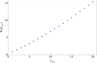
Figure 13: Plot of the behavior of $\Psi_{2}(C_{h,\alpha})$ as a function of the concentration parameter $C_{h,\alpha}$ of NFW halos.

We can use these results to determine the expected contribution of halos in a given mass-compensated void to the variance. Since total mass in halos in void $j$ is $f_{j}\Omega_{M}H_{0}^{2}R_{j}^{3}/2G$, if the fraction of this total in halos of type $\alpha$ is $\eta_{\alpha,i}$, then expected number of type $\alpha$ is

$$N_{\alpha,j}={\eta_{\alpha,i}f_{j}\Omega_{M}H_{0}^{2}Y_{j}^{3}\over 2GM_{h,\alpha}}.$$ (B17)

The expected number of intersections with type $\alpha$ is

$$\nu_{\alpha,j}={\eta_{\alpha,i}f_{j}\Omega_{M}H_{0}^{2}Y_{j}R_{h,\alpha}^{2}\over 2a_{j}^{2}GM_{h,\alpha}}.\\$$

The contribution from halos in mass-compensated void $j$ to the total variance is therefore

$${8f_{j}G\Omega_{M}H_{0}^{2}Y_{j}y_{j}^{2}(y_{S}-y_{j})^{2}\over y_{S}^{2}}\sum_{\alpha}{\eta_{\alpha,i}M_{h,\alpha}\Psi_{2}(C_{h,\alpha})\over R_{h,\alpha}^{2}}\leavevmode\nobreak\ .$$

Summing over all mass-compensated voids out to the source we get

$$\sigma^{2}_{\kappa}=\Omega_{M}\sum_{j}\left[8\sum_{\alpha}{\eta_{\alpha,i}GM_{h,\alpha}\Psi_{2}(C_{h,\alpha})\over R_{h,\alpha}^{2}}+{f_{j}\Omega_{M}H_{0}^{2}R_{i}\over 2a_{j}^{2}}\right]$$

$$\times{H_{0}^{2}Y_{j}f_{j}y_{j}^{2}(y_{S}-y_{j})^{2}\over y_{S}^{2}}\leavevmode\nobreak\ .$$

Equation (APPENDIX B: ANALYTIC ESTIMATE OF STANDARD DEVIATION) shows that the overall variance depends on halo properties primarily via the typical value of $GM_{h,\alpha}/R_{h,\alpha}^{2}$, the gravitational acceleration characteristic of the outer regions of the halo. When this is large compared with the mean gravitational acceleration of the void as a whole, $f_{j}\Omega_{M}H_{0}^{2}R_{i}/a_{j}^{2}$, the halos dominate the dispersion. There is also a hefty numerical factor $8\Psi_{2}(C_{h,\alpha})\sim 50$ favoring the contribution from halos.

If $\eta_{\alpha,i}=\eta_{\alpha}$ is actually independent of $i$ then we can factor out the sum over $\alpha$ in the first term of Eq. (APPENDIX B: ANALYTIC ESTIMATE OF STANDARD DEVIATION): define a dimensionless parameter

$${\overline{g}_{h}}\equiv{16\over H_{0}}\sum_{\alpha}{\eta_{\alpha}GM_{h,\alpha}\Psi_{2}(C_{h,\alpha})\over R_{h,\alpha}^{2}}$$

$$\;\;\;\;\;\;\;\;\;\;\;={0.175\langle M_{h,\alpha}\Psi_{2}(C_{h,\alpha})/R_{h,\alpha}^{2}\rangle\over h\times 10^{12}M_{\odot}/(300\,{\rm kpc})^{2}\times 6.84.}\\$$

We rewrite Eq. (APPENDIX B: ANALYTIC ESTIMATE OF STANDARD DEVIATION) as

$$\sigma^{2}_{\kappa}={\Omega_{M}\over 2}{\overline{g}_{h}}\sum_{j}{(H_{0}Y_{j}f_{j})H_{0}^{2}y_{j}^{2}(y_{S}-y_{j})^{2}\over y_{S}^{2}}$$

$$\;\;\;\;\;\;\;\;\;\;\;\;\;\;\;\;\;+{\Omega_{M}^{2}\over 2}\sum_{j}{(H_{0}Y_{j}f_{j})^{2}H_{0}^{2}y_{j}^{2}(y_{S}-y_{j})^{2}\over a_{j}^{2}y_{S}^{2}}.$$

The first term in Eq.(APPENDIX B: ANALYTIC ESTIMATE OF STANDARD DEVIATION) is $\sim{\overline{g}_{h}}$ and the second is $\sim\Omega_{M}H_{0}\langle Y_{j}\rangle\approx 3.5\times 10^{-3}h\langle Y_{j}\rangle/35\,{\rm Mpc}$. Eq. (APPENDIX B: ANALYTIC ESTIMATE OF STANDARD DEVIATION) suggests that halos dominate.

Now all of the parameters in Eq. (APPENDIX B: ANALYTIC ESTIMATE OF STANDARD DEVIATION) can be varied over distributions. To keep things as simple as possible, let us assume that $f_{j}$ is simply a function of redshift; that is, neglect the possible dependence of $f$ on the size of mass compensated voids. As a further simplification, we turn the sums into integrals. If we had a single void radius $R$ the sums would turn into integrals by noting that there are $dy/2R$ voids per range $dy$; for a distribution of void sizes we can use this substitution with $R_{i}\to\langle R\rangle$ in the second sum. If we also define $\xi=H_{0}y$ then with these simplifications

$$\sigma^{2}_{\kappa}(\xi_{S})={\Omega_{M}\over 4}{\overline{g}_{h}}\int_{0}^{\xi_{S}}{d\xi\,f(\xi)\xi^{2}(\xi_{S}-\xi)^{2}\over\xi_{S}^{2}}$$

$$\;\;\;\;\;\;\;\;\;\;\;\;\;\;\;\;\;\;\;+{\Omega_{M}^{2}\over 4}H_{0}\langle R\rangle\int_{0}^{\xi_{S}}{d\xi\,f^{2}(\xi)\xi^{2}(\xi_{S}-\xi)^{2}\over a^{2}(\xi)\xi_{S}^{2}}$$

The relationship between the variance of $\kappa$ and the variance of magnifications $\sigma_{m}$, for small deviations, is approximated by

$$\sigma_{m}^{2}=\left({5\over\log\left(10\right)}\right)^{2}\sigma_{\kappa}^{2}.$$

References

- (1) E. E. Flanagan, N. Kumar, I. Wasserman and R. A. Vanderveld. Phys. Rev. D , 023510 (2012).
- (2) J. Wambsganss, R. Cen, G. Xu, and J. P. Ostriker, Astron. J. Lett. , L81+ (1997).
- (3) D. E. Holz and R. M. Wald, Phys. Rev. D , 063501 (1998).
- (4) P. Valageas, Astron. Astrophys. , 767 (2000).
- (5) D.E. Holz and E. V. Linder, Ap.J. , 678 (2005).
- (6) D. Munshi et al., Phys. Rep. , 67 (2008).
- (7) R. A. Vanderveld, E. E. Flanagan, I. Wasserman. Phys Rev D , 083511 (2008).
- (8) N. Sugiura, K. Nakao, D. Ida, N. Sakai, and H. Ishihara, Prog. Theor. Phys. , 73 (2000).
- (9) T. Kai, H. Kozaki, K. Nakao, Y. Nambu, and C.-M. Yoo, Prog. Theor. Phys. , 229 (2007).
- (10) N. Brouzakis, N. Tetradis, and E. Tzavara, JCAP , 013 (2007).
- (11) K. Kainulainen, V. Marra. Phys. Rev. D , 123020 (2009).
- (12) K. Kainulainen, V. Marra. Phys. Rev. D , 023009 (2011).
- (13) J. F . Navarro, C. S. Frenk, S. D. M. White. Astrophys. J. , 563-575 (1996).
- (14) A. Nishizawa, A. Taruya, S. Saito. Phys. Rev. D , 084045 (2011).
- (15) K. Bolejko. JCAP , 025 (2011).
- (16) S. Hilbert, J. Hartlap, P. Schneider. arXiv:1105.3980v2 [astro-ph.CO].
- (17) R. Takahashi, M. Oguri, M. Sato, T. Hamana. arXiv:1106.3823v2 [astro-ph.CO].
- (18) P. Valageas, M. Sato, T. Nishimichi. arXiv:1112.1495v1 [astro-ph.CO].
- (19) T. Clifton, J. Zuntz. Mon. Not. R. Astron. Soc. , 2185 (2009).
- (20) N. Brouzakis, N. Tetradis, E. Tzavara, JCAP , 008 (2008).
- (21) S. J. Szybka. arXiv:1012.5239v1 [astro-ph.CO].
- (22) T. Biswas, A. Notari, JCAP , 021 (2008).
- (23) K. Kreckel, E. Platen, M. A. Aragn-Calvo, J. H. van Gorkom, R. van de Weygaert, J. M. van der Hulst, K. Kovac, C.-W. Yip, P. J. E. Peebles. arXiv:1008.4616v1 [astro-ph.CO]
- (24) A. Klypin, H. Zhao, R. S. Somerville, Astrophys J , 597 (2002).
- (25) X. Xue et al, Astrophys J , 1143 (2008).
- (26) V. Rashkov, P. Madau, M. Kuhlen, J. Diemand, arXiv:1106.5583v2 [astro-ph.GA].