Best-effort networks: modeling and performance analysis via large networks asymptotics

Abstract

In this paper we introduce a class of Markov models, termed best-effort networks, designed to capture performance indices such as mean transfer times in data networks with best-effort service. We introduce the so-called min bandwidth sharing policy as a conservative approximation to the classical max-min policy. We establish necessary and sufficient ergodicity conditions for best-effort networks under the min policy. We then resort to the mean field technique of statistical physics to analyze network performance deriving fixed point equations for the stationary distribution of large symmetrical best-effort networks. A specific instance of such networks is the star-shaped network which constitutes a plausible model of a network with an overprovisioned backbone. Numerical and analytical study of the equations allows us to state a number of qualitative conclusions on the impact of traffic parameters (link loads) and topology parameters (route lengths) on mean document transfer time.

1 Introduction

Consider a network handling data flows from several users, and assume no quality of service commitments (such as minimum bandwidth allocations) have been made by the network to the users. Such a situation has been prevalent in the Internet until now, and is likely to remain so for another few years.

The preferred service model in that situation, known as best effort service, consists in allocating a fair proportion of bandwidth to contending users; see, e.g., Bertsekas and Gallager [1]. There are actually several possible notions of fairness available for this bandwidth allocation problem (see, e.g., Mo and Walrand [2] for a parametric family of fairness criteria covering all other notions proposed so far), although the classical notion proposed in [1] is the so-called max-min fairness.

Recent work has led to a relatively good understanding of how bandwidth is shared between network users when a given congestion control algorithm is used; see, e.g., Massoulié and Roberts [3] and references therein. The question of what type of fairness is achieved in the current Internet, where Jacobson’s congestion avoidance algorithm—as implemented in TCP—is responsible for congestion control, has been studied in depth by Hurley et al. [4]. These studies all assume the number of flows remains fixed.

In comparison, there is little work accounting for the random nature of traffic and its impact on user perceived quality of service. Consider for instance the transfer of digital documents (Web pages, files, emails,…) using a transport protocol like TCP. This constitutes the bulk of Internet traffic today. The performance criterion relevant to such transfers is the overall document transfer time. This time is clearly highly dependent on the number of ongoing transfers on the links shared by the considered connection. This number varies as a random process as new connections are established and existing ones terminate in a way which depends on how bandwidth is allocated, as well as on the underlying traffic parameters.

In the case of a single bottleneck resource shared perfectly fairly, simple traffic assumptions of Poisson arrivals and identically and independently distributed document size lead to a processor sharing queueing model [5]. This fluid flow model provides useful results on expected response times as a function of the load of an access link or a Web server, for instance. It also shows how a form of congestion collapse can occur when demand (arrival rate $\times$ mean document size) exceeds capacity. The processor sharing queue is then no longer ergodic leading to unbounded response times. To understand the impact of multiple bottlenecks and to investigate the effect of different sharing strategies, one would like to dispose of similar analytical results for multiple resource systems.

To the best of our knowledge, the only analytical results available so far are in Massoulié and Roberts [5], where the so-called linear network topology is investigated. Simulation results for the linear network can be found both in [5] and in de Veciana et al. [6]. The main motivation for the present paper is to study the performance of best-effort networks with alternative topologies, the ultimate objective being the derivation of heuristics enabling the performance evaluation of bandwidth sharing in a general network.

In the present paper we report the results of our preliminary investigations. These include an analysis of the stability conditions under which the expected response time remains finite in a general network. We also apply mean field techniques to evaluate the performance of large symmetrical networks. Numerical results derived from the model illustrate how response times depend on the number of bottleneck links and their utilization. These results are of some practical interest and aide our understanding of the behavior of best effort networks. A further significant contribution is the insight provided into the inherent difficulty of deriving performance estimates when more than one bottleneck limits throughput.

Section 2 introduces a general class of Markov models for best-effort networks which is intended to capture the impact of network topology, traffic parameters and bandwidth sharing (fairness) criteria on document transfer times. A brief account of the results obtained in [5] is given, and the so-called “min” bandwidth allocation is introduced as a conservative approximation to max-min fairness. Section 3 then establishes the necessary and sufficient ergodicity criteria for best-effort networks under the “min” policy. Section 4 introduces the so-called “star topology”. Its relevance as a model of real networks is discussed and a mean field heuristic is proposed. This heuristic is expected to be accurate in the asymptotic regime where the number of star branches is large. The derived fixed point equations are investigated numerically in Section 5. Simulation is used to verify the accuracy of the heuristics. Extensions to the star-shaped network are also considered in Sections 4 and 5, which notably allow an evaluation of the impact of the number of bottlenecks on the mean transfer time.

2 Best-effort networks

Consider the following network model: a set ${\mathcal{L}}$ of links is given, where each link $\ell\in{\mathcal{L}}$ has an associated capacity or bandwidth $C_{\ell}>0$. A set ${\mathcal{R}}$ of routes is given, each route being identified with a subset of links. Fig. 1 illustrates the so-called linear network: it consists of $L$ links with equal capacity, route $0$ which crosses each link, and routes $r=1,\ldots,L$ which cross a single link.

To each route $r$ are associated two parameters: $\lambda_{r}$ is the arrival rate of new transfer requests along route $r$, and $\sigma_{r}$ is the average document size. We make the following standard simplifying assumptions: requests for document transfers along route $r$ arrive at the instants of a Poisson process with intensity $\lambda_{r}$, while the corresponding document sizes are mutually independent, independent of the arrival times, and drawn from an exponential distribution of mean $\sigma_{r}$.

These traffic assumptions make the process specifying the number of transfers in progress on different routes Markovian (see below) and thus greatly simplify analysis. The Poisson arrivals assumption is not unreasonable in a large network. In view of the insensitivity of performance results for an isolated link to the exact document size distribution, we do not expect divergence of the real distribution from the exponential size assumption to invalidate the derived conclusions. However, the main reason for assuming an exponential distribution is clearly one of analytical tractability.

Figure 1: The linear network

The network state is summarized by the variables $X\stackrel{{\scriptstyle\mbox{\tiny def}}}{{=}}\{x_{r},r\in{\mathcal{R}}\}$, where $x_{r}$ denotes the number of transfers in progress along route $r$. It remains to specify at what speed documents are transmitted in any given state $X$ in order to turn $X$ into a Markov process with well defined dynamics. Indeed, given the rate $\zeta_{r}(X)$ at which documents along route $r$ are transferred when the network state is $X$, $X$ is a Markov process with non-zero transition rates given by

$$\left\{\begin{array}[]{ll}x_{r}\rightarrow x_{r}+1:&\mbox{ rate }\lambda_{r},\\ x_{r}\rightarrow x_{r}-1:&\mbox{ rate }x_{r}\zeta_{r}(X)/\sigma_{r}.\end{array}\right.$$

A natural assumption would be to consider that each document receives its fair share of bandwidth. For instance, if as in [1] fairness is understood as max-min fairness, each transfer along route $r$ receives a bandwidth share $\zeta^{\text{mm}}_{r}$, where

$$\sum_{r\ni\ell}x_{r}\zeta^{\text{mm}}_{r}\leq C_{\ell},\ \forall\ell\in{\mathcal{L}},$$ (1)

and for every route $r$, there is at least one link $\ell\in r$ such that

$$\sum_{r^{\prime}\ni\ell}x_{r^{\prime}}\zeta^{\text{mm}}_{r^{\prime}}=C_{\ell},\mbox{ and }\zeta^{\text{mm}}_{r}=\max_{r^{\prime}\ni\ell}\zeta^{\text{mm}}_{r^{\prime}}.$$ (2)

These two conditions uniquely determine the bandwidth shares $\zeta^{\text{mm}}_{r}$. Having specified the Markov process $X$, one can then attempt to study its steady state properties, identifying the conditions on the load parameters

$$\rho_{\ell}\stackrel{{\scriptstyle\mbox{\tiny def}}}{{=}}\frac{1}{C_{\ell}}\sum_{r\ni\ell}\lambda_{r}\sigma_{r}$$

under which it is ergodic and, when it is, determining the stationary distribution. Mean transfer times $T_{r}$ along each route $r$ can then be computed using Little’s law: $T_{r}=\operatorname{I\!E}x_{r}/\lambda_{r}$.

It turns out that explicit formulas for steady state distributions are typically beyond reach. A notable exception is the linear network, with bandwidth shares being allocated to realize proportional rather than max-min fairness; see [5]. In order to obtain formulas in other cases, one therefore has to resort to asymptotics on various parameters. For instance, for the linear network with max-min fair rate sharing, the regime where the arrival rate $\lambda_{0}$ along route $0$ goes to zero (essentially, a form of light traffic analysis) is considered in [5]; this leads to approximate formulas for $T_{0}$. It can be shown, in particular, that $T_{0}$ increases as the logarithm of the number of links $L$ when $L$ increases. This is in contrast to the case of proportionally fair sharing where it increases linearly in $L$.

The main purpose of this paper is to investigate an alternative asymptotic regime where it is the network topology which evolves. The precise description of this limiting regime will be given in Section 4.

In the following sections, we consider bandwidth allocations according to the following “min” policy: given the network state $X$, each transfer along route $r$ receives a bandwidth share $\zeta^{\text{min}}_{r}$ given by

$$\zeta^{\text{min}}_{r}\stackrel{{\scriptstyle\mbox{\tiny def}}}{{=}}\min_{\ell\in r}\frac{C_{\ell}}{X_{\ell}},$$ (3)

where we have introduced the notation $X_{\ell}=\sum_{r^{\prime}\ni\ell}x_{r^{\prime}}$ to represent the total number of transfers making use of link $\ell$.

It is easy to check that this policy satisfies the capacity constraints (1). Moreover, it is sub-optimal with respect to the max-min fairness policy, as shown in the next theorem.

Theorem 1

Under the same initial conditions, the vector $X^{\text{mm}}(t)$ for the system under the $\zeta^{\text{mm}}$ allocation policy is stochastically smaller than $X^{\text{min}}(t)$, corresponding to the $\zeta^{\text{min}}$ allocation.

Proof 2.1.

Assume that, for some $t$, $X^{\text{mm}}(t)\leq X^{\text{min}}(t)$. Then, with the notation of (2),

$$\zeta^{\text{mm}}_{r} = \max_{r^{\prime}\ni\ell}\zeta^{\text{mm}}_{r^{\prime}}$$

$$\geq \frac{1}{X^{\text{mm}}_{\ell}(t)}\sum_{r^{\prime}\ni\ell}x^{\text{mm}}_{r^{\prime}}(t)\zeta^{\text{mm}}_{r^{\prime}}\,=\,\frac{C_{\ell}}{X^{\text{mm}}_{\ell}(t)}$$

$$\geq \frac{C_{\ell}}{X^{\text{min}}_{\ell}(t)}\,\geq\,\zeta^{\text{min}}_{r}.$$

Thus, using a coupling argument, one can define the processes $X^{\text{mm}}$ and $X^{\text{min}}(t)$ in such a way that $X^{\text{mm}}(t)\leq X^{\text{min}}(t)$ for all $t>0$.

The previous theorem motivates the study of the min policy, as it implies for instance that mean transfer times $T_{r}$ under the min policy provide upper bounds on the corresponding transfer times under the max-min policy.

3 Ergodicity conditions

In the following we demonstrate that min and max-min bandwidth sharing policies have a stationary regime under the usual conditions, i.e. when the load on each link $\ell$ is less than 1:

Theorem 2

Under the allocation policies $\zeta^{\text{mm}}$ and $\zeta^{\text{min}}$, the network is

1. ergodic if $\max_{\ell\in{\mathcal{L}}}\rho_{\ell}<1$;

2. transient if $\max_{\ell\in{\mathcal{L}}}\rho_{\ell}>1$.

This result has already been proven for the max-min policy in [6]; we note that, by Theorem 1, ergodicity under the min policy implies ergodicity under the max-min policy, thus the treatment of the min policy given below provides an alternative proof to that of [6]. However we feel that, since the proof below is simpler and uses only elementary Lyapunov functions results, it should be easier to adapt to a more complicated situation. Transience under condition (ii) is in fact valid for any allocation policy which meets the capacity constraints (1).

Proof 3.1.

Consider the discrete time chain $(\hat{X}(n),n\in{\mathrm{I\!N}})$ describing the sequence of states visited by the continuous time jump process $X$. Transitions from a given state $\hat{X}=\big{(}\hat{x}_{r},r\in{\mathcal{R}}\big{)}$ satisfy

$$\operatorname{I\!P}\bigl{[}\mathop{\Delta}\hat{x}_{r}(n)=1\bigm{|}\hat{X}(n)=\hat{X}\bigr{]} = \frac{\lambda_{r}}{D}\,,$$

$$\operatorname{I\!P}\bigl{[}\mathop{\Delta}\hat{x}_{r}(n)=-1\bigm{|}\hat{X}(n)=\hat{X}\bigr{]} = \frac{1}{D}\,\frac{\hat{x}_{r}}{\sigma_{r}}\min_{\ell\in r}\frac{C_{\ell}}{\hat{X}_{\ell}},$$

where $\mathop{\Delta}\hat{x}_{r}(n)\stackrel{{\scriptstyle\mbox{\tiny def}}}{{=}}\hat{x}_{r}(n+1)-\hat{x}_{r}(n)$ and

$$D \stackrel{{\scriptstyle\mbox{\tiny def}}}{{=}} \sum_{r\in{\mathcal{R}}}\Bigl{(}\lambda_{r}+\frac{\hat{x}_{r}}{\sigma_{r}}\min_{\ell\in r}\frac{C_{\ell}}{\hat{X}_{\ell}}\Bigr{)}$$

$$\leq |{\mathcal{R}}|\cdot\Bigl{(}\max_{r\in{\mathcal{R}}}\lambda_{r}+\max_{r\in{\mathcal{R}}}\frac{1}{\sigma_{r}}\cdot\max_{\ell\in{\mathcal{L}}}C_{\ell}\Bigr{)}$$

$$\stackrel{{\scriptstyle\mbox{\tiny def}}}{{=}} D^{\prime}.$$

Ergodicity of the continuous time process $X$ will follow from that of $\hat{X}$ and from the fact that the mean sojourn times in each state $X$ are bounded from above uniformly in $X$ (or equivalently, that the jump rates out of each state $X$ are bounded away from zero), a property which is easily verified.

Sufficient condition. Assume $\rho_{M}\stackrel{{\scriptstyle\mbox{\tiny def}}}{{=}}\max_{\ell\in{\mathcal{L}}}\rho_{\ell}<1$, and define the Lyapunov function

$$f(\hat{X})\stackrel{{\scriptstyle\mbox{\tiny def}}}{{=}}\sum_{r\in{\mathcal{R}}}\sum_{1\leq k\leq\hat{x}_{r}}\gamma_{r}^{k},$$

where $\gamma_{r}>1$ will be chosen later. The structure of the function, which may seem unnatural, has been chosen for the sake of computation; it is in fact of the general form $\sum_{r\in{\mathcal{R}}}\beta_{r}\gamma_{r}^{\hat{x}_{r}}+K$, for appropriate constants $\beta_{r}$ and $K$.

In order to express the transition rates in terms of $\hat{x}_{r}$ and $\rho_{\ell}$, remark that

$$\hat{X}_{\ell}=\sum_{r\ni\ell}\hat{x}_{r}=\sum_{r\ni\ell}\lambda_{r}\sigma_{r}\frac{\hat{x}_{r}}{\lambda_{r}\sigma_{r}}\leq\rho_{\ell}C_{\ell}\max_{r\ni\ell}\frac{\hat{x}_{r}}{\lambda_{r}\sigma_{r}}.$$

Then, using the notation

$$\hat{x}^{*}_{r}\stackrel{{\scriptstyle\mbox{\tiny def}}}{{=}}\frac{\hat{x}_{r}}{\lambda_{r}\sigma_{r}},\quad\hat{x}^{*}_{M}\stackrel{{\scriptstyle\mbox{\tiny def}}}{{=}}\max_{r\in{\mathcal{R}}}\hat{x}^{*}_{r},$$

we have, $\forall r\in{\mathcal{R}}$,

$$\operatorname{I\!P}\bigl{[}\mathop{\Delta}\hat{x}_{r}(n)=-1\bigm{|}\hat{X}(n)=\hat{X}\bigr{]}\geq\frac{\lambda_{r}}{D\rho_{M}}\frac{\hat{x}^{*}_{r}}{\hat{x}^{*}_{M}}.$$

Thus,

$$\operatorname{I\!E}\bigl{[}f(\hat{X}(n+1))-f(\hat{X}(n))\bigm{|}\hat{X}(n)=\hat{X}\bigr{]}$$

$$= \sum_{r\in{\mathcal{R}}}\Big{(}\gamma_{r}^{\hat{x}_{r}+1}\operatorname{I\!P}\bigl{[}\mathop{\Delta}\hat{x}_{r}(n)=1\bigm{|}\hat{X}(n)=\hat{X}\bigr{]}$$

$$\hphantom{\sum_{r\in{\mathcal{R}}}\Big{(}}-\gamma^{\hat{x}_{r}}\operatorname{I\!P}\bigl{[}\mathop{\Delta}\hat{x}_{r}(n)=-1\bigm{|}\hat{X}(n)=\hat{X}\bigr{]}\Big{)}$$

$$\leq \sum_{r\in{\mathcal{R}}}\frac{\lambda_{r}}{\rho_{M}D}\gamma_{r}^{\hat{x}_{r}}\Bigl{[}\rho_{M}\gamma_{r}-\frac{\hat{x}^{*}_{r}}{\hat{x}^{*}_{M}}\Bigr{]}$$

Let $\gamma_{r}\stackrel{{\scriptstyle\mbox{\tiny def}}}{{=}}\gamma^{\frac{1}{\lambda_{r}\sigma_{r}}}$, where $\gamma$ is such that

$$\rho_{M}\gamma_{r}=\rho_{M}\gamma^{\frac{1}{\lambda_{r}\sigma_{r}}}<\theta<1,\ r\in{\mathcal{R}},$$

for some real number $\theta$ satisfying $\rho_{M}<\theta<1$. The following inequality sums up what we have so far:

$$\operatorname{I\!E}\bigl{[}f(\hat{X}(n+1))-f(\hat{X}(n))\bigm{|}\hat{X}(n)=\hat{X}\bigr{]}$$

$$\leq \sum_{r\in{\mathcal{R}}}\frac{\lambda_{r}\gamma^{\hat{x}^{*}_{r}}}{\rho_{M}D}\Bigl{[}\theta-\frac{\hat{x}^{*}_{r}}{\hat{x}^{*}_{M}}\Bigr{]}.$$

Let $\alpha$ be a real number such that $\theta<\alpha<1$. The following quantities will be evaluated separately

$$\left\{\begin{array}[]{ccl}\Sigma_{1}&\stackrel{{\scriptstyle\mbox{\tiny def}}}{{=}}&\displaystyle\sum_{r:\hat{x}^{*}_{r}>\alpha\hat{x}^{*}_{M}}\frac{\lambda_{r}\gamma^{\hat{x}^{*}_{r}}}{\rho_{M}D}\Bigl{[}\theta-\frac{\hat{x}^{*}_{r}}{\hat{x}^{*}_{M}}\Bigr{]},\\[8.5359pt] \Sigma_{2}&\stackrel{{\scriptstyle\mbox{\tiny def}}}{{=}}&\displaystyle\sum_{r:\hat{x}^{*}_{r}\leq\alpha\hat{x}^{*}_{M}}\frac{\lambda_{r}\gamma^{\hat{x}^{*}_{r}}}{\rho_{M}D}\Bigl{[}\theta-\frac{\hat{x}^{*}_{r}}{\hat{x}^{*}_{M}}\Bigr{]}.\end{array}\right.$$

Since $\Sigma_{1}$ is a sum of negative terms, the following bound holds, for any $r_{0}$ is such that $\hat{x}^{*}_{r_{0}}=\hat{x}^{*}_{M}$,

$$\Sigma_{1}\leq\frac{\lambda_{r_{0}}\gamma^{\hat{x}^{*}_{M}}}{\rho_{M}D}(\theta-\alpha)\,\leq\,\frac{\gamma^{\hat{x}^{*}_{M}}}{\rho_{M}D}(\theta-\alpha)\min_{r\in{\mathcal{R}}}\lambda_{r}\,<\,0.$$

Bounding $\Sigma_{2}$ is straightforward:

$$\Sigma_{2}\leq\sum_{r:\hat{x}^{*}_{r}\leq\alpha\hat{x}^{*}_{M}}\frac{\lambda_{r}\gamma^{\alpha\hat{x}^{*}_{M}}}{\rho_{M}D}\theta\,\leq\,\frac{\gamma^{\hat{x}^{*}_{M}}}{\rho_{M}D}\gamma^{(\alpha-1)\hat{x}^{*}_{M}}|{\mathcal{R}}|\theta\max_{r\in{\mathcal{R}}}\lambda_{r}.$$

Now, if $C>0$ and $\epsilon>0$ are chosen to satisfy the inequality

$$(\theta-\alpha)\min_{r\in{\mathcal{R}}}\lambda_{r}+\gamma^{(\alpha-1)C}|{\mathcal{R}}|\theta\max_{r\in{\mathcal{R}}}\lambda_{r}\,\leq\,-\epsilon,$$

we have, $\forall\hat{X}\in\{\hat{x}^{*}_{M}>C\}$,

$$\operatorname{I\!E}\bigl{[}f(\hat{X}(n+1))-f(\hat{X}(n))\bigm{|}\hat{X}(n)=\hat{X}\bigr{]}$$

$$= \Sigma_{1}+\Sigma_{2}\,\leq\,-\epsilon\frac{\gamma^{\hat{x}^{*}_{M}}}{\rho_{M}D}\,\leq\,-\epsilon\frac{\gamma^{C}}{\rho_{M}D^{\prime}}\,<\,0.$$

Since $\{\hat{x}^{*}_{M}\leq C\}$ is a compact set, Foster’s theorem applies (see e.g. [7]) and the Markov chain is ergodic.

Necessary condition. Assume now that there exists $\ell_{0}$ such that $\rho_{\ell_{0}}>1$. Defining

$$g(\hat{X})\stackrel{{\scriptstyle\mbox{\tiny def}}}{{=}}\sum_{r\ni\ell_{0}}\sigma_{r}\hat{x}_{r},$$

we immediately have,

$$\operatorname{I\!E}\bigl{[}g(\hat{X}(n+1))-g(\hat{X}(n))\bigm{|}\hat{X}(n)=\hat{X}\bigr{]}$$

$$= \sum_{r\ni\ell_{0}}\sigma_{r}\Bigl{(}\operatorname{I\!P}\bigl{[}\mathop{\Delta}\hat{x}_{r}(n)=1\bigm{|}\hat{X}(n)=\hat{X}\bigr{]}$$

$$\hphantom{\sum_{r\ni\ell_{0}}\sigma_{r}\Bigl{[}}-\operatorname{I\!P}\bigl{[}\mathop{\Delta}\hat{x}_{r}(n)=-1\bigm{|}\hat{X}(n)=\hat{X}\bigr{]}\Bigr{)}$$

$$\geq \frac{1}{D^{\prime}}[C_{\ell_{0}}\rho_{\ell_{0}}-C_{\ell_{0}}]\,>\,0.$$

Since the jumps are bounded, the chain is transient.

4 Mean field analysis of large networks

It does not appear possible to obtain closed form expressions for the stationary distribution of the best-effort network state under the min policy. We therefore turn to the study of these stationary distributions under a limiting regime on network size and topology. A similar approach has previously been successfully applied to loss networks (see [8, 9], and references therein), and to queueing networks in [10, 11]. It is inspired by the so-called mean field models of statistical physics.

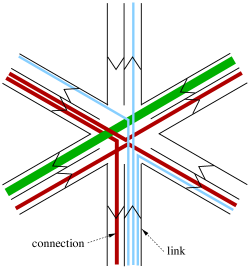
Figure 2: A star-shaped network

Mean field analysis in the present context is best illustrated by the star-shaped network of Fig. 2. This network has $N/2$ branches, each consisting of one inbound and one outbound link (thus implicitly $N$ is an even number), and all links have unit capacity. Each route $r$ connects the endpoints of two branches via the center node. It has an associated arrival rate $2\lambda/N$ and mean message length $\sigma$. The factor $2/N$ is introduced to make the total load on each link, $\rho=\lambda\sigma$, independent of the number of links $N$. As discussed below, when $N$ goes to infinity the number of ongoing transfers on any link becomes independent of the number of ongoing transfers on any finite collection of the other links (this was termed the “chaos propagation” property in [9]). This allows us to derive fixed point equations for the probability distribution of the number of transfers in progress on any link.

4.1 Symmetrical star-shaped networks

Although amenability to a mean field analysis is a significant motivation for considering the star-shaped topology, it should be noted that it is also relevant to the study of real networks. Any overprovisioned links in a real network are largely transparent to the throughput of elastic best effort flows. Only bottleneck resources, typically located in the access network and within Web servers, need to be included in the network model. The star-shaped network may thus be considered to represent any network with a well provisioned backbone where throughput is limited by bottlenecks at the source and destination edges. For example, inbound links might represent Web server CPU, while outbound links correspond to the last hop of an ISP’s interconnection network. This discussion not only motivates the consideration of such a topology, but also suggests that letting $N$ go to infinity might indeed be realistic if $N$ represents the number of Web servers over the Internet. Of course, there would be no reason in practice to assume symmetry. This assumption is introduced solely for reasons of tractability.

Although our focus is on the star-shaped topology, the mean field approach can be applied to other symmetrical topologies. It thus allows one to consider routes with more than two hops. The corresponding extended model is described in detail in Section 4.2 below, where the corresponding fixed point equations are derived. Section 4.3 then presents analytical results for the star-shaped network. Results of numerical investigation of the fixed point equations are reported in Section 5.

4.2 Fixed point equations for large symmetrical networks

We use the following notation in the sequel.

• $N$: total number of links;

• $L$: length of a route through the network;

• $R^{\scriptscriptstyle(N)}$: number of routes going through a given link;

• $X^{\scriptscriptstyle(N)}_{\ell}$: number of active connections on link $\ell\in{\mathcal{L}}$, in stationary state;

• $x^{\scriptscriptstyle(N)}_{r}$: number of active connections on route $r$, going through links $r(1),\ldots,r(L)$;

• $\lambda$: arrival rate on a link;

• $\sigma$: mean message length;

• $\rho\stackrel{{\scriptstyle\mbox{\tiny def}}}{{=}}\lambda\sigma$: load of a link.

We have implicitly assumed here that the number of routes going through a link, $R^{\scriptscriptstyle(N)}$, is the same for all links. We shall in fact assume further that the network topology is the same, as seen from any route. We do not attempt to give a formal definition of this symmetry assumption here. The reader is referred to [9] for a thorough discussion on the minimal symmetry assumptions required. Symmetry implies notably that each route has the same number of hops and the same traffic parameters. The star-shaped network discussed above constitutes an example of such a symmetrical network when $L=2$ (with $R^{\scriptscriptstyle(N)}=N/2$).

Figure 3: A hypercube-shaped network with dimension $5$.

It is more difficult to come up with meaningful examples of symmetrical networks supporting routes with $L>2$: in particular, the network should not be fully connected, since routes longer than one hop would then be pointless. One reasonable model is a hypercube (Fig. 3) of large dimension, in which each edge contains two one-way links.

The hypercube is a classical structure with many symmetries. It is characterized by its dimension $d$. Its vertices are represented by $d$-tuples of $0$s and $1$s (e.g., $(0,1,1,0,1)$) and its edges connect two vertices differing in only one coordinate.

The total number of links in such a network is $N=d2^{d}$. The number of routes going through any link is

$$R^{\scriptscriptstyle(N)}=L\frac{(d-1)!}{(d-L)!},$$

where the only routes considered are the shortest paths between two vertices which differ in exactly $L$ coordinates. Note that the results below do not depend on the precise topology of the network.

We now derive the fixed point equations. It should be stressed that this derivation is heuristic. We clearly mention which steps need further justification in the course of the derivation. We do believe that the equations are very good approximations, however, especially in view of the numerical and simulation results presented in the following section.

Assume now that $\rho<1$ and that the system is in stationary state $X^{\scriptscriptstyle(N)}=(x^{\scriptscriptstyle(N)}_{r},r\in{\mathcal{R}})$. For any $k\geq 0$, the proportion of links in state $k$ is

$$\alpha^{\scriptscriptstyle(N)}_{k}\stackrel{{\scriptstyle\mbox{\tiny def}}}{{=}}\frac{1}{N}\sum_{\ell\in{\mathcal{L}}}\leavevmode\hbox{{\small 1\kern-3.15005pt\normalsize 1}}_{\{X^{\scriptscriptstyle(N)}_{\ell}=k\}}.$$

By symmetry, it holds that

$$\operatorname{I\!P}(X^{\scriptscriptstyle(N)}_{\ell}=k)=\operatorname{I\!E}\alpha^{\scriptscriptstyle(N)}_{k},\ \forall\ell\in{\mathcal{L}}.$$

The chaos propagation assumption implies that $\alpha^{\scriptscriptstyle(N)}_{k}$ obeys a law of large numbers:

$$\alpha_{k}\stackrel{{\scriptstyle\mbox{\tiny def}}}{{=}}\lim_{N\to\infty}\alpha^{\scriptscriptstyle(N)}_{k}=\lim_{N\to\infty}\operatorname{I\!P}(X^{\scriptscriptstyle(N)}_{\ell}=k)\stackrel{{\scriptstyle\mbox{\tiny def}}}{{=}}\operatorname{I\!P}(X=k).$$

It appears that the dynamics of the system are driven by $\alpha^{\scriptscriptstyle(N)}_{k}$, traditionally referred to as the mean field. The following notation will also be useful:

$${\bar{\alpha}}^{\scriptscriptstyle(N)}\stackrel{{\scriptstyle\mbox{\tiny def}}}{{=}}\sum_{k>0}k\alpha^{\scriptscriptstyle(N)}_{k},\qquad{\bar{\alpha}}\stackrel{{\scriptstyle\mbox{\tiny def}}}{{=}}\operatorname{I\!E}X_{\ell}=\sum_{k>0}k\alpha_{k}.$$

In order to derive the equation satisfied by the limit stationary distribution $\alpha_{k}$, we must first describe the possible transitions for $\alpha^{\scriptscriptstyle(N)}_{k}$. The two cases of interest are

• arrival on a link with $k$ connections:

  $$\alpha^{\scriptscriptstyle(N)}_{k}\to\alpha^{\scriptscriptstyle(N)}_{k}-\frac{1}{N},\quad\alpha^{\scriptscriptstyle(N)}_{k+1}\to\alpha^{\scriptscriptstyle(N)}_{k+1}+\frac{1}{N}$$

• departure from a link with $k>0$ connections:

  $$\alpha^{\scriptscriptstyle(N)}_{k}\to\alpha^{\scriptscriptstyle(N)}_{k}-\frac{1}{N},\quad\alpha^{\scriptscriptstyle(N)}_{k-1}\to\alpha^{\scriptscriptstyle(N)}_{k-1}+\frac{1}{N}$$

The transition corresponding to a new connection arrival has rate $\lambda$. The main problem is to compute the departure rate from a link $\ell$, given that it has $X^{\scriptscriptstyle(N)}_{\ell}=k$ ongoing transfers. This can be written as

$$\frac{1}{\sigma}\sum_{r\ni\ell}\operatorname{I\!E}\Bigl{[}x^{\scriptscriptstyle(N)}_{r}\min_{\ell^{\prime}\in r}\frac{1}{X^{\scriptscriptstyle(N)}_{r(\ell^{\prime})}}\Bigm{|}X^{\scriptscriptstyle(N)}_{\ell}=k\Bigr{]}.$$ (4)

Since the total number of routes is much larger than the size $N$ of the network, we assume that the probability of having more than one connection on a route $r$ is negligible, and that the links on route $r$ are independent, conditioned on $\{x^{\scriptscriptstyle(N)}_{r}=1\}$. The first property allows to rewrite (4) as

$$\frac{1}{\sigma}\sum_{r\ni\ell}\operatorname{I\!E}[x^{\scriptscriptstyle(N)}_{r}\mid X^{\scriptscriptstyle(N)}_{\ell}=k]\operatorname{I\!E}\Bigl{[}\min_{\ell^{\prime}\in r}\frac{1}{X^{\scriptscriptstyle(N)}_{r(\ell^{\prime})}}\Bigm{|}x^{\scriptscriptstyle(N)}_{r}=1\Bigr{]}.$$ (5)

Let $j$ be a given link and let $r$ be one route using link $j$, i.e., $r\ni j$. The distribution of $X^{\scriptscriptstyle(N)}_{j}$, conditioned on there being one connection on $r$, is then

$$\operatorname{I\!P}\bigl{[}X^{\scriptscriptstyle(N)}_{j}=k^{\prime}\bigm{|}x^{\scriptscriptstyle(N)}_{r}=1\bigr{]}=\frac{\operatorname{I\!E}\bigl{[}\leavevmode\hbox{{\small 1\kern-3.15005pt\normalsize 1}}_{\{X^{\scriptscriptstyle(N)}_{j}=k^{\prime}\}}\leavevmode\hbox{{\small 1\kern-3.15005pt\normalsize 1}}_{\{x^{\scriptscriptstyle(N)}_{r}=1\}}\bigr{]}}{\operatorname{I\!E}\leavevmode\hbox{{\small 1\kern-3.15005pt\normalsize 1}}_{\{x^{\scriptscriptstyle(N)}_{r}=1\}}}.$$

By symmetry, it is possible to sum both sides of the above fraction over all the routes going through link $j$,

$$\operatorname{I\!P}\bigl{[}X^{\scriptscriptstyle(N)}_{j}=k^{\prime}\bigm{|}x^{\scriptscriptstyle(N)}_{r}=1\bigr{]} = \frac{\operatorname{I\!E}\bigl{[}X^{\scriptscriptstyle(N)}_{j}\leavevmode\hbox{{\small 1\kern-3.15005pt\normalsize 1}}_{\{X^{\scriptscriptstyle(N)}_{j}=k^{\prime}\}}\bigr{]}}{\operatorname{I\!E}X^{\scriptscriptstyle(N)}_{j}}$$

$$= \frac{k^{\prime}\operatorname{I\!E}\alpha^{\scriptscriptstyle(N)}_{k^{\prime}}}{\operatorname{I\!E}{\bar{\alpha}}^{\scriptscriptstyle(N)}}.$$

Departure rate (5) then becomes, in view of the assumed independence property between the $X_{r(i)}$ given $x_{r}=1$,

$$\frac{k}{\sigma}\sum_{k_{2},\ldots,k_{L}=1}^{\infty}\biggl{(}\frac{1}{k}\wedge\frac{1}{k_{2}}\wedge\cdots\wedge\frac{1}{k_{L}}\biggr{)}\prod_{i=2}^{L}\frac{k_{i}\operatorname{I\!E}\alpha^{\scriptscriptstyle(N)}_{k_{i}}}{\operatorname{I\!E}{\bar{\alpha}}^{\scriptscriptstyle(N)}}.$$

Taking the limit $N\to\infty$, the invariant measure equations follow. We have:

$$-\lambda\alpha_{0}+\frac{1}{\sigma}\alpha_{1}\frac{u_{1}}{{\bar{\alpha}}^{L-1}}=0$$ (6)

and

$$\lambda(\alpha_{k-1}-\alpha_{k})+\frac{1}{\sigma}\left(\alpha_{k+1}\frac{u_{k+1}}{{\bar{\alpha}}^{L-1}}-\alpha_{k}\frac{u_{k}}{{\bar{\alpha}}^{L-1}}\right)=0$$ (7)

for $k\geq 1$, where

$$u_{k}\,\stackrel{{\scriptstyle\mbox{\tiny def}}}{{=}}\,k\sum_{k_{2},\ldots k_{L}=1}^{\infty}\biggl{(}\frac{1}{k}\wedge\frac{1}{k_{2}}\wedge\cdots\wedge\frac{1}{k_{L}}\biggr{)}\prod_{i=2}^{L}k_{i}\alpha_{k_{i}}.$$ (8)

Equations (6) and (7) can be rewritten in a more concise form as

$$\alpha_{k+1}u_{k+1}=\rho{\bar{\alpha}}^{L-1}\alpha_{k},\qquad\forall k\geq 0.$$ (9)

The two sets of equations (8) and (9) together constitute the fixed point equations we require. As noted in the introduction of this section, these equations do not depend on the topology of the network. The expression for $u_{k}$ can be simplified.

Let $Y_{2},\ldots,Y_{L}$ be random variables with distribution

$$\operatorname{I\!P}(Y_{i}=y)=\frac{y\alpha_{y}}{{\bar{\alpha}}},\ 2\leq i\leq L,$$

and let $Y\stackrel{{\scriptstyle\mbox{\tiny def}}}{{=}}\max(Y_{2},\ldots,Y_{L})$. Then (8) reads

$$u_{k}\,=\,k{\bar{\alpha}}^{L-1}\,\operatorname{I\!E}\Bigl{[}\frac{1}{k}\wedge\frac{1}{Y}\Bigr{]}.$$ (10)

Straightforward calculations yield

$$\operatorname{I\!E}\Bigl{[}\frac{1}{k}\wedge\frac{1}{Y}\Bigr{]} = \sum_{y=1}^{\infty}\Bigl{[}\frac{1}{k}\wedge\frac{1}{y}\Bigr{]}\operatorname{I\!P}(Y=y)$$

$$= \sum_{y=k}^{\infty}\frac{1}{y(y+1)}\operatorname{I\!P}(Y\leq y).$$

The simplified form for $u_{k}$ is thus, from the basic properties of the minimum of independent random variables:

$$u_{k}\,=\,k\sum_{y=k}^{\infty}\frac{1}{y(y+1)}\Bigl{[}\sum_{m=0}^{y}m\alpha_{m}\Bigr{]}^{L-1}.$$ (11)

Note that, in the case $L=2$ (i.e., for the star-shaped network), the original equation (8) is perhaps simpler than the equivalent expression (11). It yields the following form for the fixed point equations:

$$\alpha_{k+1}u_{k+1} = \rho{\bar{\alpha}}\alpha_{k},$$ (12)

$$u_{k} = \sum_{y>0}(k\wedge y)\alpha_{y}.$$ (13)

Remark 4.1.

When considering the star-shaped network as a model for Web transfers over the Internet, as suggested in Section 4.1, inbound links could be seen as the CPU of Web servers and outbound links as the last hop between the ISP’s backbone and the end customers. It thus makes sense to relax the symmetry assumption we had made between inbound and outbound links, as the two types of bottlenecks are of a different nature. We might thus consider a star-shaped network with $N^{\mbox{\tiny in}}$ inbound links, $N^{\mbox{\tiny out}}$ outbound links, inbound (resp. outbound) links having capacity $C^{\mbox{\tiny in}}$ (resp. $C^{\mbox{\tiny out}}$), see Fig. 4. Assume the mean message length $\sigma$ is the same for each two-hop route, and the link capacities $C^{\mbox{\tiny out}}$ are fixed. The arrival rate on each route has the form $\lambda_{r}\stackrel{{\scriptstyle\mbox{\tiny def}}}{{=}}\lambda/N^{\mbox{\tiny in}}$, and the load $\rho^{\mbox{\tiny out}}\stackrel{{\scriptstyle\mbox{\tiny def}}}{{=}}\lambda\sigma/C^{\mbox{\tiny out}}$ is less that $1$. The capacity $C^{\mbox{\tiny in}}$ of a “backbone” link is chosen to ensure $\rho^{\mbox{\tiny in}}\stackrel{{\scriptstyle\mbox{\tiny def}}}{{=}}\lambda\sigma N^{\mbox{\tiny out}}/C^{\mbox{\tiny in}}N^{\mbox{\tiny in}}<1$ is fixed when the size of the system grows. Then, as $N^{\mbox{\tiny in}}$ and $N^{\mbox{\tiny out}}$ increase, with $N^{\mbox{\tiny in}}/N^{\mbox{\tiny out}}$ small, the inbound links have many active connections and a large capacity, while the outbound links remain in “normal” utilization. The same approach as above can then be applied, to yield the set of fixed point equations

$$\alpha_{k+1}^{\mbox{\tiny in}}u_{k+1}^{\mbox{\tiny out}} = \rho^{\mbox{\tiny in}}{\bar{\alpha}}^{\mbox{\tiny out}}\alpha_{k}^{\mbox{\tiny in}},$$

$$\alpha_{k+1}^{\mbox{\tiny out}}u_{k+1}^{\mbox{\tiny in}} = \rho^{\mbox{\tiny in}}{\bar{\alpha}}^{\mbox{\tiny out}}\alpha_{k}^{\mbox{\tiny out}},$$

where

$$u_{k}^{\mbox{\tiny in}} = \sum_{y>0}\alpha^{\mbox{\tiny in}}_{y}\min\Bigl{[}k,\frac{C^{\mbox{\tiny out}}}{C^{\mbox{\tiny in}}}y\Bigr{]},$$

$$u_{k}^{\mbox{\tiny out}} = \sum_{y>0}\alpha^{\mbox{\tiny out}}_{y}\min\Bigl{[}\frac{C^{\mbox{\tiny out}}}{C^{\mbox{\tiny in}}}k,y\Bigr{]},$$

and $\alpha_{k}^{\mbox{\tiny in}}$ (resp. $\alpha_{k}^{\mbox{\tiny out}}$) represents the proportion of inbound (resp. outbound) links with $k$ ongoing transfers.

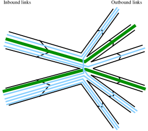
Figure 4: The asymmetrical star-shaped network

4.3 Analytical results for $L=2$

While equation (9) looks superficially like a “birth and death process” equation, it is in fact non-linear due to the fact that $u_{k}$ and ${\bar{\alpha}}$ both depend on the $\alpha_{y}$.

From (10), one clearly sees that $u_{k}$ is increasing in $k$, and tends to ${\bar{\alpha}}^{L-1}$ when $k\to\infty$. Therefore, $\alpha_{k}$ is increasing as long as $u_{k}<\rho{\bar{\alpha}}^{L-1}$, and decreasing after that. This means that the $\alpha_{k}$ form a modal distribution, which maximal value is attained at

$$k_{0}=\max\{k>0,\ u_{k}<\rho{\bar{\alpha}}^{L-1}\}.$$

We now present analytical results on the solution of the fixed point equations for $L=2$. The proof of these results can be found in [12]. It relies heavily on functional analysis.

Equations (12)–(13) have an unique solution for $\rho<1$ and, when $\rho\to 1$, the following asymptotic expansions hold:

$$\operatorname{I\!E}X \approx \frac{1}{(1-\rho)^{2}A},$$

$$\lim_{k\to\infty}\rho^{-k}\operatorname{I\!P}(X=k) \approx (1-\rho)B\exp\Bigl{[}\frac{1}{(1-\rho)A}\Bigr{]},$$

where $A$ and $B$ are non-negative constants.

Thus, under the min policy, any link in the star-shaped network has a mean queue length which is one order of magnitude larger than for a single server queue with the same load ($\rho/(1-\rho)$). Its tail distribution is still geometrical with factor $\rho$.

It is possible to give an expression for the constant $A$: if $c$ and $v$ are solutions of the following system of differential equations,

$$\begin{cases}zc^{\prime}(z)+c(z)v(z)=0,\\ zv^{\prime\prime}(z)+v^{\prime}(z)=c(z),\\ v(0)=0,\quad v^{\prime}(0)=1,\quad c(0)=1,\end{cases}$$

then $A$ can be written as follows:

$$A=\int_{0}^{\infty}c(z)dz=\lim_{z\to\infty}zv^{\prime}(z)\approx 1.30.$$

Since this system is numerically highly unstable, it has proven difficult (with the “Livermore stiff ODE” solver from MAPLE) to derive a better estimate for $A$.

It is interesting to note that the function $w(y)\stackrel{{\scriptstyle\mbox{\tiny def}}}{{=}}v(e^{y})+1$ satisfies the so-called Blasius [13] equation

$$w^{\prime\prime\prime}(y)+w(y)w^{\prime\prime}(y)=0,$$

which describes a laminar boundary layer along a flat plate (see, e.g., [14]).

5 Numerical analysis and simulations

Figure 5: Distribution of the mean-field probabilities $\operatorname{I\!P}(X=k)$ for $L=20$ and different values of the load $\rho$.

While the analytical results of Section 4.3 give some good estimates, they are only valid in the heavy traffic regime $\rho\to 1$. In addition, similar results for $L>2$ are not available. We thus resort to numerical resolution of the equations to gain a better understanding of the performance of transfers across large symmetrical networks. The very form of the equations suggests the use of a fixed-point method for this numerical resolution: starting from a priori values $(\alpha_{k}^{\scriptscriptstyle(0)},k\geq 0)$, the algorithm computes the corresponding $u_{k}^{\scriptscriptstyle(0)}$ from (8), and then new values $\alpha_{k}^{\scriptscriptstyle(1)}$ from (9). Provided special care is taken to avoid instabilities, the iteration of this process converges rapidly (less than $100$ steps). Sample results are shown in Fig. 5, corresponding to a large symmetrical network with routes of length $L=20$.

As clearly seen in the figure, the distributions are very different from what would be obtained for routes of length $L=1$. In this case, the system consists of a collection of independent M/M/$1$ queues and the associated distribution $\{\alpha_{k}\}$ is geometric. For $L>1$, the $\{\alpha_{k}\}$ distributions are markedly modal and the positions of the peak values are roughly proportional to $(1-\rho)^{-2}$, a fact has only been proven in Section 4.3 for the case $L=2$. Moreover, since the shape of the distribution is rather narrow, this position roughly coincides with the mean number of active connection (as can be seen from the raw data).

Figure 6: Distribution of the mean-field probabilities $\operatorname{I\!P}(X=k)$ for different values of the route length $L$ and load $\rho=0.9$.

The impact of route length is illustrated in Fig. 6. It seems that the mean number of active connections (which is again approximately the peak value of the distribution) is roughly proportional to $\log L$. Note that a logarithmic growth rate is very slow suggesting that, beyond 2 or 3, the number of bottlenecks does not have a significant impact on mean transfer times. They depend much more on the load $\rho$.

The results presented so far only concern the solution of the fixed point equations. As mentioned earlier, there are gaps in the derivation of these equations. To assess their quality and to investigate the accuracy of the asymptotic approximation for finite size networks, we ran a number of simulations of the star-shaped network. Fig. 7 displays the corresponding results when the load on each link is set to $\rho=0.9$ for a varying number of links. The agreement between the simulation results and the fixed point equation results is excellent for $N=100$ links and improves as $N$ increases.

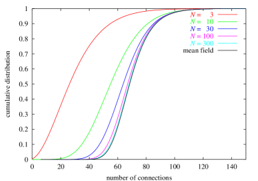
Figure 7: Cumulative distribution $\operatorname{I\!P}(X\leq k)$ for different values of $N$ (simulation) and infinite size (fixed point) for a star-shaped network with load $\rho=0.9$.

6 Conclusions

In this paper, we have considered a class of Markov processes called best-effort networks which constitutes a natural probabilistic model for evaluating the performance of document transfers over data networks such as the Internet. Unlike almost all previous work, this model accounts for the random nature of traffic: document transfers begin at the epochs of a certain arrival process and the size of each document is drawn from a given probability distribution. In the interests of tractability we assumed Poisson arrivals and exponentially distributed sizes. We introduced the “min” bandwidth sharing policy as a conservative approximation to the more classical max-min policy. Necessary and sufficient ergodicity conditions for best effort networks under the min and max-min policies have been established.

In order to pursue the analysis of the stationary distributions of the number of transfers in progress, we have resorted to large network asymptotics applying the mean field approach of statistical physics. This enabled us to derive fixed point equations for the probability distribution of the number of ongoing transfers on a given network link. The validity of these equations has been established by comparing their solution with the results of simulations.

Analytical and numerical results show how the mean transfer time depends on the number of bottleneck links and their load. The steady state distribution in networks where routes have several bottlenecks ($L>1$) has a marked modal behavior. This is significantly different to the geometric distribution which holds when routes have a single bottleneck ($L=1$). Performance is also much more sensitive to link load $\rho$ for multiple bottleneck routes: as $\rho\to 1$, mean transfer time increases like $1/(1-\rho)^{2}$ in the case $L=2$, whereas the dependence is in $1/(1-\rho)$ when $L=1$. Finally, the impact of the number of hops per route $L$ appears small (given that $L>1$) compared to that of parameter $\rho$. This suggests that the star-shaped network is perhaps a sufficiently complex model, and that the study of symmetrical networks with $L>2$ is less relevant.

The work presented here can be pursued in several directions. On the theoretical side, the analytical results presented in Section 4.3 constitute a first step to understanding the solution of the fixed point equations which could be taken further. Another challenging theoretical question is to improve the fixed point equations in a rigorous way. On a more practical side, the fixed point equations might be simplified so as to find simple approximate formulas for mean transfer times as a function of key parameters (such as $\rho^{\mbox{\tiny{in}}}$, $\rho^{\mbox{\tiny{out}}}$ in the case of the asymmetrical star-shaped network described in Remark 4.1). Such approximate formulas could then lead to engineering rules for capacity planning.

We view the present study as a preliminary investigation into the performance of best effort networks with multiple bottleneck links. A significant result of this investigation is the discovery that the extension of the processor sharing model valid for a single bottleneck proves to be very hard. There appears to be no simple parallel to the familiar fixed point techniques used in loss networks. The problem is, however, of considerable practical importance for providers seeking to engineer their network to ensure adequate throughput for document transfers. We hope therefore that this paper will incite further work and the development of alternative heuristic approaches.

References

- [1] D. Bertsekas and R. Gallager, Data Networks, Prentice-Hall International, 2nd edition, 1992.
- [2] J. H. Mo and J. Walrand, “Fair end-to-end window-based congestion control,” in SPIE ’98 International Symposium on Voice,Video and Data Communications, 1998.
- [3] L. Massoulié and J. Roberts, “Bandwidth sharing: objectives and algorithms,” IEEE Infocom, 1999.
- [4] P. Hurley, J.-Y. Leboudec, and P. Thiran, “A note on the fairness of additive increase and multiplicative decrease,” ITC 16, 1999.
- [5] J. Roberts and L. Massoulié, “Bandwidth sharing and admission control for elastic traffic,” ITC specialists seminar, 1998.
- [6] G. De Veciana, T.-J. Lee, and T. Konstantopoulos, “Stability and performance analysis of networks supporting services with rate control – could the internet be unstable?,” IEEE Infocom, 1999.
- [7] G. Fayolle, V. A. Malyshev, and M. V. Menshikov, Topics in the Constructive Theory of Countable Markov Chains, Cambridge University Press, 1995.
- [8] F. Kelly, “Loss networks,” Ann. Appl. Probab., vol. 1, pp. 319–378, 1991.
- [9] C. Graham and S. Méléard, “Chaos hypothesis for a system interacting through shared resources,” Probability Theory and Related Fields, 1994.
- [10] N. D. Vvedenskaya, R. L. Dobrushin, and F. I. Karpelevich, “A queueing system with a choice of the shorter of two queues—an asymptotic approach,” Problems Inform. Transmission, vol. 32, pp. 15–27, 1996.
- [11] F. Delcoigne and G. Fayolle, “Thermodynamical limit and propagation of chaos in polling systems,” Markov Processes and Related Fields, vol. 5, no. 1, pp. 89–124, 1999.
- [12] G. Fayolle and J.-M. Lasgouttes, “A nonlinear integral operator encountered in the bandwidth sharing of a star-shaped network,” in Mathematics and Computer Science: Algorithms, Trees, Combinatorics and Probabilities, Trends in Mathematics, pp. 231–242. Birkha ser, 2000.
- [13] H. Blasius, “Grenzschichten in flüssigkeiten mit kleiner reibung,” Z. Math Phys., vol. 56, pp. 1–37, 1908, English translation in NACA TM 1256.
- [14] H. Schlichting, Boundary layer theory, McGraw-Hill Book Co., Inc., New York, 1960, Translated by J. Kestin. 4th ed. McGraw-Hill Series in Mechanical Engineering.