Kernel Principal Component Analysis and its Applications in
Face Recognition and Active Shape Models
Abstract
Principal component analysis (PCA) is a popular tool for linear dimensionality reduction and feature extraction. Kernel PCA is the nonlinear form of PCA, which better exploits the complicated spatial structure of high-dimensional features. In this paper, we first review the basic ideas of PCA and kernel PCA. Then we focus on the reconstruction of pre-images for kernel PCA. We also give an introduction on how PCA is used in active shape models (ASMs), and discuss how kernel PCA can be applied to improve traditional ASMs. Then we show some experimental results to compare the performance of kernel PCA and standard PCA for classification problems. We also implement the kernel PCA-based ASMs, and use it to construct human face models.
1 Introduction
In this section, we briefly review the principal component analysis method and the active shape models.
1.1 Principal Component Analysis
Principal component analysis, or PCA, is a very popular technique for dimensionality reduction and feature extraction. PCA attempts to find a linear subspace of lower dimensionality than the original feature space, where the new features have the largest variance (Bishop, 2006).
Consider a dataset where , and each is a -dimensional vector. Now we want to project the data onto an -dimensional subspace, where . We assume the projection is denoted as , where , and for . We want to maximize the variance of , which is the trace of the covariance matrix of . Thus, we want to find
| (1) |
where
| (2) |
and
| (3) |
Let be the covariance matrix of . Since , by using the Lagrangian multiplier and taking the derivative, we get
| (4) |
which means that is an eigenvector of . Now can be represented as
| (5) |
can be also approximated by
| (6) |
where is the eigenvector of corresponding to the th largest eigenvalue.
1.2 Active Shape Models
The active shape model, or ASM, is one of the most popular top-down object fitting approaches. It is designed to represent the complicated deformation patterns of the object shape, and to locate the object in new images. ASMs use the point distribution model (PDM) to describe the shape (Cootes et al., 1995). If a shape consists of points, and denotes the coordinates of the th point, then the shape can be represented as a -dimensional vector
| (7) |
To simplify the problem, we now assume that all shapes have already been aligned. Otherwise, a rotation by , a scaling by , and a translation by should be applied to . Given aligned shapes as training data, the mean shape can be calculated by
| (8) |
For each shape in the training set, its deviation from the mean shape is
| (9) |
Then the covariance matrix can be calculated by
| (10) |
Now we perform PCA on :
| (11) |
where is the eigenvector of corresponding to the th largest eigenvalue , and
| (12) |
Let be the matrix of the first eigenvectors:
| (13) |
Then we can approximate a shape in the training set by
| (14) |
where is the vector of weights for different deformation patterns. By varying the parameters , we can generate new examples of the shape. We can also limit each to constrain the deformation patterns of the shape. Typical limits are
| (15) |
where . Another important issue of ASMs is how to search for the shape in new images using point distribution models. This problem is beyond the scope of our paper, and here we only focus on the statistical model itself.
2 Kernel PCA
Standard PCA only allows linear dimensionality reduction. However, if the data has more complicated structures which cannot be well represented in a linear subspace, standard PCA will not be very helpful. Fortunately, kernel PCA allows us to generalize standard PCA to nonlinear dimensionality reduction (Schölkopf et al., 1999).
2.1 Constructing the Kernel Matrix
Assume we have a nonlinear transformation from the original -dimensional feature space to an -dimensional feature space, where usually . Then each data point is projected to a point . We can perform standard PCA in the new feature space, but this can be extremely costly and inefficient. Fortunately, we can use kernel methods to simplify the computation (Schölkopf et al., 1998).
First, we assume that the projected new features have zero mean:
| (16) |
The covariance matrix of the projected features is , calculated by
| (17) |
Its eigenvalues and eigenvectors are given by
| (18) |
where . From Eq. (17) and Eq. (18), we have
| (19) |
which can be rewritten as
| (20) |
Now by substituting in Eq. (19) with Eq. (20), we have
| (21) |
If we define the kernel function
| (22) |
and multiply both sides of Eq. (21) by , we have
| (23) |
We can use the matrix notation
| (24) |
where
| (25) |
and is the -dimensional column vector of :
| (26) |
can be solved by
| (27) |
and the resulting kernel principal components can be calculated using
| (28) |
If the projected dataset does not have zero mean, we can use the Gram matrix to substitute the kernel matrix . The Gram matrix is given by
| (29) |
where is the matrix with all elements equal to (Bishop, 2006).
The power of kernel methods is that we do not have to compute explicitly. We can directly construct the kernel matrix from the training data set (Weinberger et al., 2004). Two commonly used kernels are the polynomial kernel
| (30) |
or
| (31) |
where is a constant, and the Gaussian kernel
| (32) |
with parameter .
The standard steps of kernel PCA dimensionality reduction can be summarized as:
2.2 Reconstructing Pre-Images
So far, we have discussed how to generate new features using kernel PCA. This is enough for applications such as feature extraction and data classification. However, for some other applications, we need to approximately reconstruct the pre-images from the kernel PCA features . This is the case in active shape models, where we not only need to use PCA features to describe the deformation patterns, but also have to reconstruct the shapes from the PCA features (Romdhani et al., 1999; Twining & Taylor, 2001).
In standard PCA, the pre-image can simply be approximated by Eq. (6). However, Eq. (6) cannot be used for kernel PCA (Gökhan H. Bakır et al., 2004). For kernel PCA, we define a projection operator which projects to its approximation
| (33) |
where is the eigenvector of the matrix, which is define by Eq. (17). If is large enough, we have . Since finding the exact pre-image is difficult, we turn to find an approximation such that
| (34) |
This can be approximated by minimizing
| (35) |
2.3 Pre-Images for Gaussian Kernels
There are some existing techniques to compute for specific kernels (Mika et al., 1999). For a Gaussian kernel , should satisfy
| (36) |
where
| (37) |
We can compute iteratively:
| (38) |
3 Experiments
In this section, we show the setup and results of our three experiments. The first two experiments are classification problems without pre-image reconstruction. The third experiment combines active shape models with kernel PCA, and involves the pre-image reconstruction algorithm.
3.1 Pattern Classification for Synthetic Data
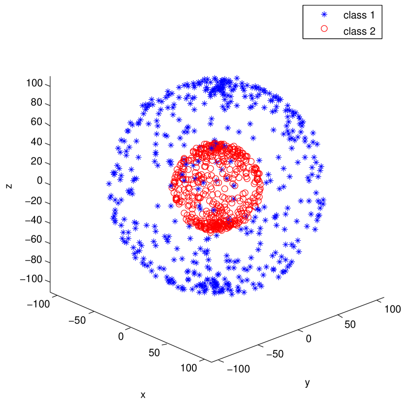
Before we work on real data, we would like to generate some synthetic datasets and test our algorithm on them. In this paper, we use the two-concentric-spheres data.
3.1.1 Data Description
We assume that we have equal numbers or data points distributed on two concentric sphere surfaces. If is the total number of all data points, then we have class 1 points on a sphere of radius , and class 2 points on a sphere of radius . In the spherical coordinate system, the inclination (polar angle) is uniformly distributed in , and the azimuth (azimuthal angle) is uniformly distributed in for both classes. Our observations of the data points are the coordinates in the Cartesian coordinate system, and all the three coordinates are perturbed by a Gaussian noise of standard deviation . We set , , , , and give a 3D plot of the data in Figure 1.
3.1.2 PCA and Kernel PCA Results
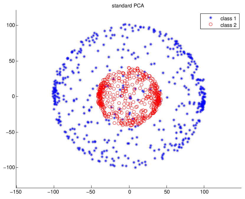
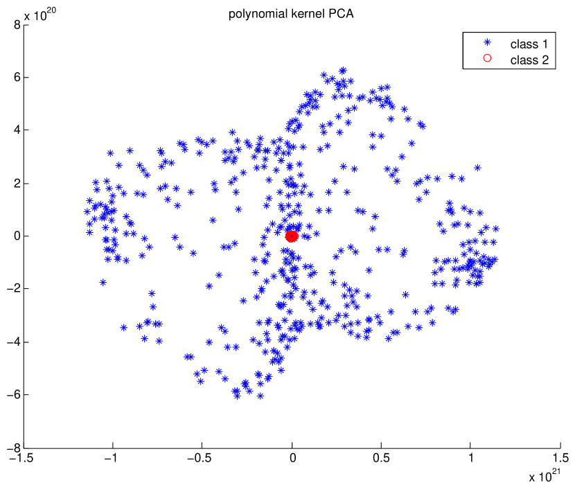
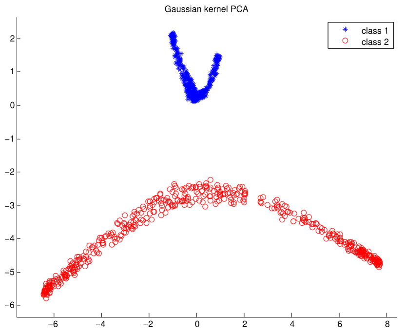
To visualize our results, we project the original 3-dimensional data onto a 2-dimensional feature space by using both standard PCA and kernel PCA. For kernel PCA, we use a polynomial kernel with , and a Gaussian kernel with (parameter selection is discussed in Section 4). The results of standard PCA, polynomial kernel PCA, and Gaussian kernel PCA are given in Figure 2, Figure 3, and Figure 4, respectively.
We note that here though we mark points in different classes with different colors, we are actually doing unsupervised learning. Neither standard PCA nor kernel PCA takes the class labels as their input.
In the resulting figures we can see that, standard PCA does not reveal any structural information of the original data. For polynomial kernel PCA, in the new feature space, class 2 data points are clustered while class 1 data points are scattered. But they are still not linearly separable. For Gaussian kernel PCA, the two classes are completely linearly separable.
3.2 Classification for Aligned Human Face Images
After we have tested our algorithm on synthetic data, we would like to use it for real data classification. Here we use PCA and kernel PCA to extract features from human face images, and use the simplest linear classifier (Krzanowski, 2000) for classification. Then we compare the error rates of using PCA and kernel PCA.
3.2.1 Data Description
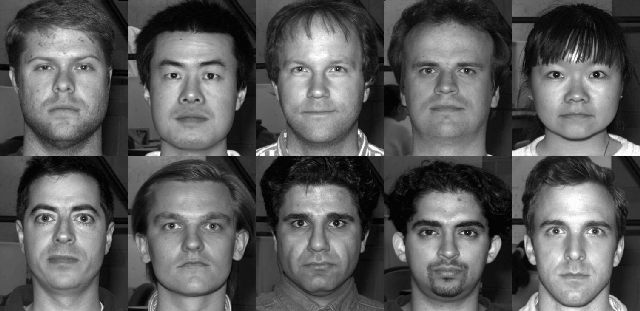
For this task, we use images from the Yale Face Database B (Georghiades et al., 2001), which contains 5760 single light source gray-level images of 10 subjects, each seen under 576 viewing conditions. We take 51 images of the first subject and 51 images of the third subject as the training data, and 13 images of each of them as testing data. Then all the images are aligned, and each image has pixels. Example images of the Yale Face Database B are shown in Figure 5.
3.2.2 Classification Results
We use the pixel intensities as the original features for each image, thus the original feature vector is -dimensional. Then we use standard PCA and Gaussian kernel PCA to extract the 9 most significant features from the training data, and record the eigenvectors.
For standard PCA, only the eigenvectors are needed to extract features from testing data. For Gaussian kernel PCA, both the eigenvectors and the training data are needed to extract features from testing data. Note that for standard PCA, there are particular fast algorithms to compute the eigenvectors when the dimensionality is much higher than the number of data points (Bishop, 2006).
For kernel PCA, we use a Gaussian kernel with (we will talk about how to select the parameters in Section 4). For classification, we use the simplest linear classifier (Krzanowski, 2000). The training error rates and the testing error rates for standard PCA and Gaussian kernel PCA are given in Table 1. We can see that Gaussian kernel PCA achieves much lower error rates than standard PCA.
| Error Rate | PCA | Kernel PCA |
|---|---|---|
| Training Data | 8.82% | 6.86% |
| Testing Data | 23.08% | 11.54% |
3.3 Kernel PCA-Based Active Shape Models
In ASMs, the shape of an object is described with point distribution models, and standard PCA is used to extract the principal deformation patterns from the shape vectors . If we use kernel PCA instead of standard PCA here, it is promising that we will be able to discover more hidden deformation patterns.
3.3.1 Data Description
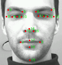
In our work, we use Tim Cootes’ manually annotated points of 1521 human face images from the BioID database. For each face image, 20 feature points (landmarks) are annotated, as shown in Figure 6. Thus the original feature vector for each image is -dimensional (two coordinates for each landmark).
3.3.2 Experimental Results
In our work, we first normalize all the shape vectors by restricting both the coordinates and coordinates in the range . Then we perform standard PCA and Gaussian kernel PCA on the normalized shape vectors. For standard PCA, the reconstruction of the shape is given by
| (39) |
For kernel PCA, the reconstruction of the shape is given by
| (40) |
where denotes the reconstruction algorithm described by Eq. (38).
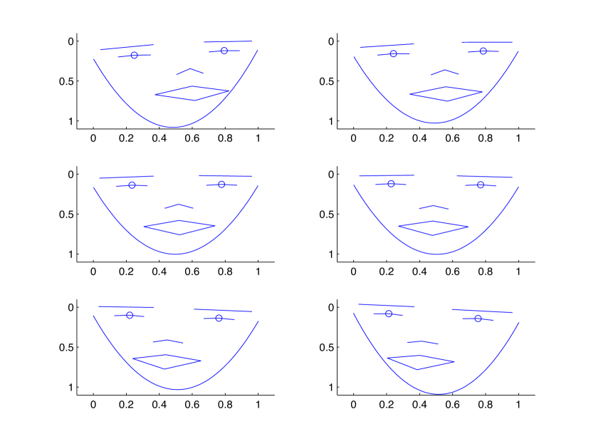
For standard PCA, we focus on studying the deformation pattern associated with each entry of . That is to say, each time we uniformly select different values of in , and set for all . The effects of varying the first PCA feature, the second PCA feature, and the third PCA feature are shown in Figure 7, Figure 8 and Figure 9, respectively. The face is drawn by using line segments to represent eye brows, eyes, the nose, using circles to represent eye balls, using a quadrilateral to represent the mouth, and fitting a parabola to represent the contour of the face.
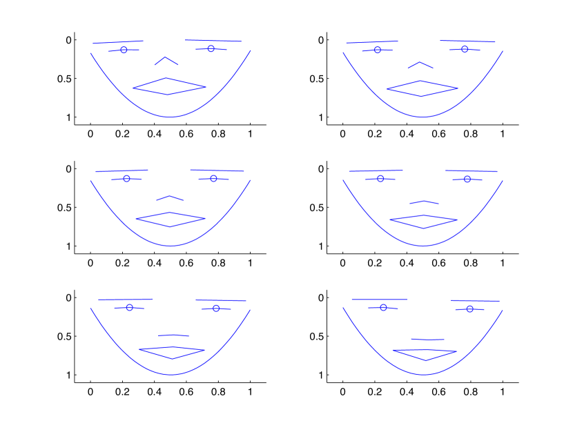

For Gaussian kernel PCA, we set for the Gaussian kernel (the parameter selection method will be given in Section 4). To study the effects of each feature extracted with kernel PCA, we compute the mean and the standard deviation of all the kernel PCA features. Each time, we uniformly sample in the range , where is a constant, and set for all . When , the effects of varying the first Gaussian kernel PCA feature, the second Gaussian kernel PCA feature, and the third Gaussian kernel PCA feature are shown in Figure 10, Figure 11 and Figure 12, respectively.
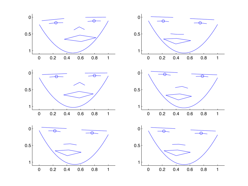
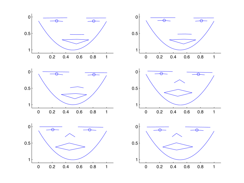
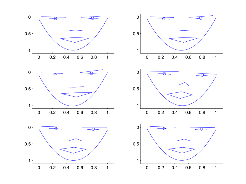
By observation, we can see that the first PCA feature affects the orientation of the human face (left or right), and the second PCA feature to some extent determines some microexpression from amazement to calmness of the human face. In contrast, the Gaussian kernel PCA features seem to be determining some very different microexpressions than PCA features.
4 Discussions
In this section, we address two concerns: First, how do we select the parameters for Gaussian kernel PCA; Second, what is the intuitive explanation of Gaussian kernel PCA.
4.1 Parameter Selection
Parameter selection for kernel PCA directly determines the performance of the algorithm. For Gaussian kernel PCA, the most important parameter is the in the kernel function defined by Eq. (32). The Gaussian kernel is a function of the distance between two vectors and . Ideally, if we want to separate different classes in the new feature space, then the parameter shoud be smaller than inter-class distances, and larger than inner-class distances. However, we don’t know how many classes are there in the data, thus it is not easy to estimate the inter-class or inner class distances. Alternatively, we can set to a small value to capture only the neighborhood information of each data point. For this purpose, for each data point , let the distance from to its nearest neighbor be . In our experiments, we use this parameter selection strategy:
| (41) |
This strategy, in our experiments, ensures that the is large enough to capture neighboring data points, and is much smaller than inter-class distances. When using different datasets, this strategy may need modifications.
For the pre-image reconstruction of Gaussian kernel PCA, the initial guess will determine whether the iterative algorithm (38) converges. We can always simply use the mean of the training data as the initial guess:
| (42) |
4.2 Intuitive Explanation of Gaussian Kernel PCA
We can see that in our synthetic data classification experiment, Gaussian kernel PCA with a properly selected parameter can perfectly separate the two classes in an unsupervised manner, which is impossible for standard PCA. In the human face images classification experiment, Gaussian kernel PCA has a lower training error rate and a much lower testing error rate than standard PCA. From these two experiments, we can see that Gaussian kernel PCA reveals more complex hidden structures of the data than standard PCA. An intuitive understanding of the Gaussian kernel PCA is that it makes use of the distances between different training data points, which is like -nearest neighbor or clustering methods. With a well selected , Gaussian kernel PCA will have a proper capture range, which will enhance the connection between data points that are close to each other in the original feature space. Then by applying eigenvector analysis, the eigenvectors will describe the directions in a high-dimensional space in which different clusters of data are scattered to the greatest extent.
In this paper we are mostly using Gaussian kernel for kernel PCA. This is because it is intuitive, easy to implement, and possible to reconstruct the pre-images. However, we indicate that there are techniques to find more powerful kernel matrices by learning-based methods (Weinberger et al., 2004, 2005).
5 Conclusion
In this paper, we discussed the theories of PCA, kernel PCA and ASMs. Then we focused on the pre-image reconstruction for Gaussian kernel PCA, and used this technique to design kernel PCA-based ASMs. We tested kernel PCA dimensionality reduction on synthetic data and human face images, and found that Gaussian kernel PCA succeeded in revealing more complicated structures of data than standard PCA, and achieving much lower classification error rates. We also implemented the Gaussian kernel PCA-based ASM and tested it on human face images. We found that Gaussian kernel PCA-based ASMs are promising in providing more deformation patterns than traditional ASMs. A potential application is that we could combine traditional ASMs and Gaussian kernel PCA-based ASMs for microexpression recognition on human face images. Besides, we proposed a parameter selection method to find the proper parameters for Gaussian kernel PCA, which works well in our experiments.
Acknowledgment
The author would like to thank Johan Van Horebeek (horebeek@cimat.mx) and Flor Martinez (flower10@cimat.mx) from CIMAT for reviewing our code and reporting the bugs.
References
- Bishop (2006) Bishop, Christopher M. (ed.). Pattern Recognition and Machine Learning. Springer, Cambridge, U.K., 2006.
- Cootes et al. (1995) Cootes, Timothy F, Taylor, Christopher J, Cooper, David H, and Graham, Jim. Active shape models — their training and application. Computer vision and image understanding, 61(1):38–59, 1995.
- Demers & Y (1993) Demers, David and Y, Garrison Cottrell. Non-linear dimensionality reduction. In Advances in Neural Information Processing Systems 5, pp. 580–587. Morgan Kaufmann, 1993.
- Georghiades et al. (2001) Georghiades, A.S., Belhumeur, P.N., and Kriegman, D.J. From few to many: Illumination cone models for face recognition under variable lighting and pose. IEEE Transactions on Pattern Analysis and Machine Intelligence, 23(6):643–660, 2001.
- Gökhan H. Bakır et al. (2004) Gökhan H. Bakır, Weston, Jason, and Schölkopf, Bernhard. Learning to find pre-images. In Advances in Neural Information Processing Systems, pp. 449–456. MIT Press, 2004.
- Krzanowski (2000) Krzanowski, Wojtek J. Principles of multivariate analysis. Clarendon, 2000.
- Mika et al. (1999) Mika, Sebastian, Schölkopf, Bernhard, Smola, Alex, Müller, Klaus-Robert, Scholz, Matthias, and Rätsch, Gunnar. Kernel pca and de-noising in feature spaces. In Advances in Neural Information Processing Systems 11, pp. 536–542. MIT Press, 1999.
- Romdhani et al. (1999) Romdhani, Sami, Gong, Shaogang, Psarrou, Ahaogang, et al. A multi-view nonlinear active shape model using kernel pca. In BMVC, volume 10, pp. 483–492, 1999.
- Schölkopf et al. (1998) Schölkopf, Bernhard, Smola, Alexander, and Müller, Klaus-Robert. Nonlinear component analysis as a kernel eigenvalue problem. Neural computation, 10(5):1299–1319, 1998.
- Schölkopf et al. (1999) Schölkopf, Bernhard, Smola, Alexander, and Müller, Klaus-Robert. Kernel principal component analysis. In Advances in Kernel Methods – Support Vector Learning, pp. 327–352. MIT Press, 1999.
- Twining & Taylor (2001) Twining, C. J. and Taylor, C. J. Kernel principal component analysis and the construction of non-linear active shape models. In Proceedings of British Machine Vision Conference, pp. 23–32, 2001.
- Weinberger et al. (2004) Weinberger, Kilian Q., Sha, Fei, and Saul, Lawrence K. Learning a kernel matrix for nonlinear dimensionality reduction. In Proceedings of the 21st International Conference on Machine Learning (ICML-04), pp. 839–846. ACM Press, 2004.
- Weinberger et al. (2005) Weinberger, Kilian Q., Packer, Benjamin D., and Saul, Lawrence K. Nonlinear dimensionality reduction by semidefinite programming and kernel matrix factorization. In Proceedings of the Tenth International Workshop on Artificial Intelligence and Statistics, pp. 381–388, 2005.