$\Sigma_{b}\to\Sigma_{c}$ and $\Omega_{b}\to\Omega_{c}$ weak decays in the light-front quark model

Abstract

The successful operation of LHC provides a great opportunity to study the processes where heavy baryons are involved. In this work we mainly study the weak transitions of $\Sigma_{b}\to\Sigma_{c}$. Assuming the reasonable quark-diquark structure where the two light quarks constitute an axial vector, we calculate the widths of semi-leptonic decay $\Sigma_{b}\to\Sigma_{c}e\nu_{e}$ and non-leptonic decay modes $\Sigma_{b}\to\Sigma_{c}+M$ (light mesons) in terms of the light front quark model. We first construct the vertex function for the concerned baryons and then deduce the form factors which are related to two Isgur-Wise functions for the $\Sigma_{b}\to\Sigma_{c}$ transition under the heavy quark limit. Our numerical results indicate that $\Gamma(\Sigma_{b}\to\Sigma_{c}e\nu_{e})$ is about $1.38\times 10^{10}{\rm s}^{-1}$ and $\Gamma(\Sigma_{b}\to\Sigma_{c}+M)$ is slightly below $1\times 10^{10}{\rm s}^{-1}$ which may be accessed at the LHCb detector. By the flavor SU(3) symmetry we estimate the rates of $\Omega_{b}\to\Omega_{c}$. We suggest to measure weak decays of $\Omega_{b}\to\Omega_{c}$, because $\Omega_{b}$ does not decay via strong interaction, the advantage is obvious.

I Introduction

In our previous work Ke:2007tg , we investigated the transitions between heavy baryons $\Lambda_{b}\to\Lambda_{c}$ by assuming the baryonic heavy-quark-light-diquark structures in terms of the Light-Front-Quark model (LFQM). The results are reasonably consistent with the available data, so it implies that the whole scenario is realistic in that case, however still needs more studies on its validity in other cases. As noticed that the ground state diquarks in $\Lambda_{b}$ and $\Lambda_{c}$ are color-anti-triplet scalars. In this work, we continue to consider the transitions of $\Sigma_{b}\to\Sigma_{c}$ because the ground state diquark in $\Sigma_{b(c)}$ is an axial vector. We explore if the difference of the diquark identities would result in distinct behaviors for the transitions and then by comparing with data we are able to gain more insight about the diquark structure.

Thanks to the successful operation of LHC, a remarkable database on baryons, especially on the heavy baryons will be available at LHCb. It enables researchers to closely study the properties of heavy baryons at their production and decay processes.

Since the situation is confronting a radical change, more physicists are turning to concern baryons and look for hints of new physics. For example, as the decay $\Sigma\rightarrow p\,\mu^{+}\,\mu^{-}$ was observedPark:2005eka the authors of Ref.He:2006fr ; He:2005we studied contribution from new physics candidates by analyzing the data. However, as it is well known when one explores possible new physics scenario based on the data, he needs to fully understand the contribution of the standard model (SM) i.e. before attributing the phenomena to new physics a complete analysis on the SM contribution is necessary.

In this work we explore the weak transition of $\Sigma_{b}\rightarrow\Sigma_{c}$. The dominant strong decay mode $\Sigma_{b}\rightarrow\Lambda_{b}+\pi$ determines the lifetime of $\Sigma_{b}$, thus the weak decays of $\Sigma_{b}$ are rare. However, from another aspect, the rare decays of $\Sigma_{b}$ may be more sensitive to new physics, so that it is worth a careful study.

Supposing the factorization is valid, the transition between quarks would be fully described by the perturbative theory and calculable, thus the main task for studying $\Sigma_{b}\rightarrow\Sigma_{c}$ is to deal with the hadronic transition matrix element. The hadronic matrix elements are determined by non-perturbative QCD and are generally parameterized by some form factors which can be reduced into a few equivalent Isgur-Wise functions under the heavy quark limitIW . Some authors Korner:1992uw ; Ebert:2006rp ; Singleton:1990ye ; Ivanov:1996fj ; Ivanov:1998ya calculated the form factors of the transition $\Sigma_{b}\rightarrow\Sigma_{c}$ in various approaches.

The quark-diquark structure that heavy baryons are made of a heavy quark and a light diquarkwilczek ; GKLLW ; yu is generally considered as a reasonable physics picture for heavy baryons. With the quark-diquark structure the authors of Refs.Korner:1992uw ; Ebert:2006rp ; Ke:2007tg ; Wei:2009np evaluated the transition rates between heavy baryons and their results are consistent with the available data. It is noted that the diquark stands as a spectator in the transition of $\Sigma_{b}\rightarrow\Sigma_{c}$, so that under the heavy quark limit, the spin of light diquark decouples and we may evaluate the rates of the corresponding rare decays in terms of the Isgur-Wise functions. A general analysis suggests that there exist many Isgur-Wise-type functions for a transition between baryons Guo and usually it would be hard to determine them by fitting data. However, with the quark-diquark structure, the number of such functions for the transition $\Sigma_{b}\to\Sigma_{c}$ reduces into only two.

The light-front quark model (LFQM) is a relativistic quark model which has been applied to study transitions among mesons and the results agree with the data within reasonable error tolerance Jaus ; Ji:1992yf ; Cheng:1996if ; Cheng:2003sm ; Hwang:2006cua ; Li:2010bb ; Ke:2009ed ; Wei:2009nc ; Choi:2007se , thus we would be tempted to extend its application to calculate the transition of $\Sigma_{b}\rightarrow\Sigma_{c}$ as long as the diquark picture is employed. In Ref.Ke:2007tg we calculated the transition of $\Lambda_{b}\rightarrow\Lambda_{c}$ in terms of LFQM. In that work we first constructed the vertex function of $\Lambda_{b(c)}$ and then deduced the form factors for the transition. However the formulas in Ke:2007tg do not apply to the decay $\Sigma_{b}\rightarrow\Sigma_{c}$ because the diquark in $\Lambda_{b(c)}$ is a scalar of color-anti-triplet, but that in $\Sigma_{b(c)}$ is an axial vector as discussed in Refs.Korner:1992uw ; Ebert:2006rp . Thus we need to re-construct the vertex function for a $\frac{1}{2}^{+}$ heavy baryon which is regarded as a bound state of a heavy quark and a light axial vector diquark. Then with the vertex functions of baryons we would derive the transition matrix element which are parametrized by a few form factors, and under the heavy quark limit, we will show that the transition matrix element of $\Sigma_{b}\to\Sigma_{c}$ can be described by two generalized Isgur-Wise functions. Numerically the results obtained in the two approaches are rather close, so it implies that the employed approaches are reasonably consistent with the physical picture.

Since the leptons do not participate in the strong interaction, the semileptonic decay is simple and less contaminated by the non-perturbative QCD effect, therefore study on semileptonic decay might help to test the employed model and/or constrain the model parameters. With the form factors we evaluate the width of the semileptonic decay. Comparing our numerical result with data the model parameters which are hidden in the vertex functions can be fixed. Moreover, the amplitude of the non-leptonic decay $\Sigma_{b}\rightarrow\Sigma_{c}+M$ can also be evaluated in a similar way as long as we suppose that the meson current can be factorized out. Moreover, we further investigate the transitions of $\Omega_{b}\to\Omega_{c}$ by assuming the flavor SU(3) symmetry. Since $\Omega_{b}$ does not decay via strong interaction, the weak decays are dominant, so that study on such modes has an obvious advantage.

This paper is organized as follows: after the introduction, in section II we construct the vertex functions of heavy baryons, then derive the form factors for the transition $\Sigma_{b}\rightarrow\Sigma_{c}$ in the light-front quark model, then we present our numerical results for the transition $\Sigma_{b}\rightarrow\Sigma_{c}$ along with all necessary input parameters in section III, then we also evaluate the transition of $\Omega_{b}\to\Omega_{c}$. Section IV is devoted to our conclusion and discussions.

II $\Sigma_{b}\rightarrow\Sigma_{c}$ in the light-front quark model

By the quark-diquark structureKorner:1992uw ; Ebert:2006rp , the heavy baryon $\Sigma_{b(c)}$ consists of a light $1^{+}$ diquark [ud] and one heavy quark $b(c)$. To insure the quantum number of $\Sigma_{b(c)}$, the orbital angular momentum between the two components is zero, i.e. $l=0$.

II.1 the vertex function of $\Sigma_{b(c)}$

In analog to our previous work Ke:2007tg , we construct the vertex function of $\Sigma_{Q}$ ($Q=b,c$) where the diquark is an axial vector in the same model. The wavefunction of $\Sigma_{Q}$ with total spin $S=1/2$ and momentum $P$ is

$$|\Sigma_{Q}(P,S,S_{z})\rangle = \int\{d^{3}\tilde{p}_{1}\}\{d^{3}\tilde{p}_{2}\}\,2(2\pi)^{3}\delta^{3}(\tilde{P}-\tilde{p_{1}}-\tilde{p_{2}})$$ (1)

$$\times\sum_{\lambda_{1}}\Psi^{SS_{z}}(\tilde{p}_{1},\tilde{p}_{2},\lambda_{1})C^{\alpha}_{\beta\gamma}F^{bc}\left|\right.Q_{\alpha}(p_{1},\lambda_{1})[q_{1b}^{\beta}q_{2c}^{\gamma}](p_{2})\rangle,$$

with

$$\Psi^{SS_{z}}(\tilde{p}_{1},\tilde{p}_{2},\lambda_{1},\lambda_{2})= \left\langle\lambda_{1}\left|\mathcal{R}^{\dagger}_{M}(x_{1},k_{1\perp},m_{1})\right|s_{1}\right\rangle\left\langle\lambda_{2}\left|\mathcal{R}^{\dagger}_{M}(x_{2},k_{2\perp},m_{2})\right|s_{2}\right\rangle$$

$$\left\langle\frac{1}{2}s_{1};1s_{2}\left|\frac{1}{2}S_{z}\right\rangle\varphi(x,k_{\perp})\right.,$$

where $\langle\frac{1}{2}s_{1};1s_{2}|\frac{1}{2}S_{z}\rangle$ is the C-G coefficients and $s_{1},s_{2}$ are the spin projections of the constituents (the heavy quark and diquark). A Melosh transformation brings the the matrix elements from the spin-projection-on-fixed-axes representation into the helicity representation and is explicitly written as

$$\left\langle\lambda_{2}\left|\mathcal{R}^{\dagger}_{M}(x_{2},k_{2\perp},m_{2})\right|s_{2}\right\rangle=\xi^{*}(\lambda_{1},m_{2})\cdot\xi(s_{2},m_{2}),$$

and

$$\left\langle\lambda_{1}\left|\mathcal{R}^{\dagger}_{M}(x_{1},k_{1\perp},m_{1})\right|s_{1}\right\rangle=\frac{\bar{u}(k_{1},\lambda_{1})u(k_{1},s_{1})}{2m_{1}}.$$

Following Refs. Jaus ; Cheng:2003sm , the Melosh transformed matrix can be expressed as

$$\left\langle\lambda_{2}\left|\mathcal{R}^{\dagger}_{M}(x_{2},k_{2\perp},m_{2})\right|s_{2}\right\rangle\left\langle\lambda_{1}\left|\mathcal{R}^{\dagger}_{M}(x_{1},k_{1\perp},m_{1})\right|s_{1}\right\rangle\left\langle\frac{1}{2}s_{1};1s_{2}\left|\frac{1}{2}S_{z}\right\rangle\right.$$

$$=\frac{1}{\sqrt{2(p_{1}\cdot\bar{P}+m_{1}M_{0})}}\bar{u}(p_{1},\lambda_{1})\Gamma u(\bar{P},S_{z}),$$ (2)

where

$$\Gamma=-\frac{1}{\sqrt{3}}\gamma_{5}\varepsilon^{*}\!\!\!\!\!\!/\;(p_{2},\lambda_{2}),\qquad m_{1}=m_{Q},\qquad m_{2}=m_{[ud]},\qquad\bar{P}=p_{1}+p_{2},$$ (3)

and

$$\varphi(x,k_{\perp})=A\phi,$$ (4)

with $\phi=4(\frac{\pi}{\beta^{2}})^{3/4}\frac{e_{1}e_{2}}{x_{1}x_{2}M_{0}}{\rm exp}(\frac{-\mathbf{k}^{2}}{2\beta^{2}})$ and $A=\sqrt{\frac{12(M_{0}m_{1}+p_{1}\cdot\bar{P})}{12M_{0}m_{1}+4p_{1}\bar{P}+8p_{1}\cdot p_{2}p_{2}\cdot\bar{P}/m_{2}^{2}}}$ which can be obtained by normalizing the state $|\Sigma_{Q}(P,S,S_{z})\rangle$ ,

$$\langle\Sigma_{Q}(P^{\prime},S^{\prime},S^{\prime}_{z})|\Sigma_{Q}(P,S,S_{z})\rangle=2(2\pi)^{3}P^{+}\delta^{3}(\tilde{P}^{\prime}-\tilde{P})\delta_{S^{\prime}S}\delta_{S^{\prime}_{z}S_{z}}.$$ (5)

All other notations can be found in Ref.Ke:2007tg .

II.2 $\Sigma_{b}\to\Sigma_{c}$ transition form factors

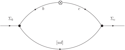
Figure 1: Feynman diagram for $\Sigma_{b}\to\Sigma_{c}$ transitions, where $\bigotimes$ denotes $V-A$ current vertex.

The lowest order Feynman diagram for the $\Sigma_{b}\to\Sigma_{c}$ weak decay is shown in Fig. 1.

Using the wavefunction for $\mid\Sigma_{Q}(P,S,S_{z})\rangle$, we obtain

$$\langle\Sigma_{Q^{\prime}}(P^{\prime},S_{z}^{\prime})\mid\bar{Q}^{\prime}\gamma^{\mu}(1-\gamma_{5})Q\mid\Sigma_{Q}(P,S_{z})\rangle$$ (6)

$$= \int\{d^{3}\tilde{p}_{2}\}\frac{\phi_{\Sigma_{Q^{\prime}}}^{*}(x^{\prime},k^{\prime}_{\perp})\phi_{\Sigma_{Q}}(x,k_{\perp})}{2\sqrt{p^{+}_{1}p^{\prime+}_{1}(p_{1}\cdot\bar{P}+m_{1}M_{0})(p^{\prime}_{1}\cdot\bar{P^{\prime}}+m^{\prime}_{1}M^{\prime}_{0})}}$$

$$\times\bar{u}(\bar{P^{\prime}},S^{\prime}_{z})\bar{\Gamma}^{\prime}(p_{1}\!\!\!\!\!/^{\prime}+m^{\prime}_{1})\gamma^{\mu}(1-\gamma_{5})(p_{1}\!\!\!\!\!/+m_{1})\Gamma u(\bar{P},S_{z}),$$

where

$$\bar{\Gamma}^{\prime}=\gamma_{0}\Gamma^{\prime}\gamma_{0},$$

$$m_{1}=m_{b},\qquad m^{\prime}_{1}=m_{c},\qquad m_{2}=m_{[ud]},$$ (7)

and $Q$($Q^{\prime}$) represent $b$($c$) quark, $p_{1}$($p^{\prime}_{1}$) is its momentum and $P$($P^{\prime}$) denotes the momentum of initial (final) baryon. From $\tilde{p}_{2}=\tilde{p}^{\prime}_{2}$, we have

$$x^{\prime}=\frac{P^{+}}{P^{{}^{\prime}+}}x,\qquad\qquad k^{\prime}_{\perp}=k_{\perp}+x_{2}q_{\perp}.$$ (8)

with $x=x_{2}$, $x^{\prime}=x^{\prime}_{2}$. Thus, Eq. (6) is rewritten as

$$\langle\Sigma_{Q^{\prime}}(P^{\prime},S_{z}^{\prime})\mid\bar{Q}^{\prime}\gamma^{\mu}(1-\gamma_{5})Q\mid\Sigma_{Q}(P,S_{z})\rangle$$ (9)

$$= \int\frac{dxd^{2}k_{\perp}}{2(2\pi)^{3}}\frac{\phi_{\Sigma_{Q^{\prime}}}(x^{\prime},k^{\prime}_{\perp})\phi_{\Sigma_{Q}}(x,k_{\perp})}{2\sqrt{x_{1}x^{\prime}_{1}(p_{1}\cdot\bar{P}+m_{1}M_{0})(p^{\prime}_{1}\cdot\bar{P^{\prime}}+m^{\prime}_{1}M^{\prime}_{0})}}$$

$$\times\bar{u}(\bar{P^{\prime}},S^{\prime}_{z})[\frac{1}{\sqrt{3}}\gamma_{5}\varepsilon(\lambda_{2}^{\prime})^{*}](p_{1}\!\!\!\!\!/^{\prime}+m^{\prime}_{1})\gamma^{\mu}(1-\gamma_{5})(p_{1}\!\!\!\!\!/+m_{1})[\frac{1}{\sqrt{3}}\gamma_{5}\varepsilon(\lambda_{2})]u(\bar{P},S_{z}).$$

The form factors for the weak transition $\Sigma_{Q}\rightarrow\Sigma_{Q^{\prime}}$ are defined in the standard way as

$$\langle\Sigma_{Q^{\prime}}(P^{\prime},S^{\prime},S_{z}^{\prime})\mid\bar{Q}^{\prime}\gamma_{\mu}(1-\gamma_{5})Q\mid\Sigma_{Q}(P,S,S_{z})\rangle$$ (10)

$$= \bar{u}_{\Sigma_{Q^{\prime}}}(P^{\prime},S^{\prime}_{z})\left[\gamma_{\mu}f_{1}(q^{2})+i\sigma_{\mu\nu}\frac{q^{\nu}}{M_{\Sigma_{Q}}}f_{2}(q^{2})+\frac{q_{\mu}}{M_{\Sigma_{Q}}}f_{3}(q^{2})\right]u_{\Sigma_{Q}}(P,S_{z})$$

$$-\bar{u}_{\Sigma_{Q^{\prime}}}(P^{\prime},S^{\prime}_{z})\left[\gamma_{\mu}g_{1}(q^{2})+i\sigma_{\mu\nu}\frac{q^{\nu}}{M_{\Sigma_{Q}}}g_{2}(q^{2})+\frac{q_{\mu}}{M_{\Sigma_{Q}}}g_{3}(q^{2})\right]\gamma_{5}u_{\Sigma_{Q}}(P,S_{z}).$$

where $q\equiv P-P^{\prime}$, $Q$ and $Q^{\prime}$ denote $b$ and $c$, respectively. Since $S=S^{\prime}=1/2$, we will be able to write $\mid\Sigma_{Q}(P,S,S^{\prime}_{z})\rangle$ as $\mid\Sigma_{Q}(P,S_{z})\rangle$.

FollowingKe:2007tg ; pentaquark2 , we extract the form factors for the weak transition matrix elements of $\Sigma_{b}\to\Sigma_{c}$ as

$$f_{1}(q^{2}) = \frac{1}{8P^{+}P^{\prime+}}\int{\frac{dx_{2}d^{2}k_{2\perp}}{2(2\pi)^{3}}}\frac{\phi^{\prime*}_{00}(x^{\prime},k^{\prime}_{\perp})\phi_{00}(x,k_{\perp})}{6\sqrt{x_{1}x^{\prime}_{1}(p_{1}\cdot\bar{P}+m_{1}M_{0})(p^{\prime}_{1}\cdot\bar{P^{\prime}}+m^{\prime}_{1}M^{\prime}_{0})}}$$

$$Tr[(\bar{P}\!\!\!\!/+M_{0})\gamma^{+}(\bar{P^{\prime}}\!\!\!\!\!\!/+M^{\prime}_{0})\gamma_{5}\gamma_{a}(p_{1}\!\!\!\!\!/^{\prime}+m^{\prime}_{1})\gamma^{+}(p_{1}\!\!\!\!\!/+m_{1})\gamma_{5}\gamma_{b}](\frac{p_{2}^{a}p_{2}^{b}}{m_{2}^{2}}-g^{ab})$$

$$g_{1}(q^{2}) = \frac{1}{8P^{+}P^{\prime+}}\int{\frac{dx_{2}d^{2}k_{2\perp}}{2(2\pi)^{3}}}\frac{\phi^{\prime*}_{00}(x^{\prime},k^{\prime}_{\perp})\phi_{00}(x,k_{\perp})}{6\sqrt{x_{1}x^{\prime}_{1}(p_{1}\cdot\bar{P}+m_{1}M_{0})(p^{\prime}_{1}\cdot\bar{P^{\prime}}+m^{\prime}_{1}M^{\prime}_{0})}}$$

$$Tr[(\bar{P}\!\!\!\!/+M_{0})\gamma^{+}\gamma_{5}(\bar{P^{\prime}}\!\!\!\!\!\!/+M^{\prime}_{0})\gamma_{5}\gamma_{a}(p_{1}\!\!\!\!\!/^{\prime}+m^{\prime}_{1})\gamma^{+}\gamma_{5}(p_{1}\!\!\!\!\!/+m_{1})\gamma_{5}\gamma_{b}](\frac{p_{2}^{a}p_{2}^{b}}{m_{2}^{2}}-g^{ab})$$

$$\frac{f_{2}(q^{2})}{M_{\Lambda_{Q}}} = -\frac{1}{8P^{+}P^{\prime+}q^{i}_{\perp}}\int{\frac{dx_{2}d^{2}k_{2\perp}}{2(2\pi)^{3}}}\frac{\phi^{\prime*}_{00}(x^{\prime},k^{\prime}_{\perp})\phi_{00}(x,k_{\perp})}{6\sqrt{x_{1}x^{\prime}_{1}(p_{1}\cdot\bar{P}+m_{1}M_{0})(p^{\prime}_{1}\cdot\bar{P^{\prime}}+m^{\prime}_{1}M^{\prime}_{0})}}$$

$$Tr[(\bar{P}\!\!\!\!/+M_{0})\sigma^{i+}(\bar{P^{\prime}}\!\!\!\!\!\!/+M^{\prime}_{0})\gamma_{5}\gamma_{a}(p_{1}\!\!\!\!\!/^{\prime}+m^{\prime}_{1})\gamma^{+}(p_{1}\!\!\!\!\!/+m_{1})\gamma_{5}\gamma_{b}](\frac{p_{2}^{a}p_{2}^{b}}{m_{2}^{2}}-g^{ab})$$

$$\frac{g_{2}(q^{2})}{M_{\Lambda_{Q}}} = \frac{1}{8P^{+}P^{\prime+}q^{i}_{\perp}}\int{\frac{dx_{2}d^{2}k_{2\perp}}{2(2\pi)^{3}}}\frac{\phi^{\prime*}_{00}(x^{\prime},k^{\prime}_{\perp})\phi_{00}(x,k_{\perp})}{6\sqrt{x_{1}x^{\prime}_{1}(p_{1}\cdot\bar{P}+m_{1}M_{0})(p^{\prime}_{1}\cdot\bar{P^{\prime}}+m^{\prime}_{1}M^{\prime}_{0})}}$$ (11)

$$Tr[(\bar{P}\!\!\!\!/+M_{0})\sigma^{i+}\gamma_{5}(\bar{P^{\prime}}\!\!\!\!\!\!/+M^{\prime}_{0})\gamma_{5}\gamma_{a}(p_{1}\!\!\!\!\!/^{\prime}+m^{\prime}_{1})\gamma^{+}\gamma_{5}(p_{1}\!\!\!\!\!/+m_{1})\gamma_{5}\gamma_{b}](\frac{p_{2}^{a}p_{2}^{b}}{m_{2}^{2}}-g^{ab}).$$

with $i=1,2$. The traces can be worked out straightforwardly and all the details can be found in Ref.Ke:2007tg .

II.3 Isgur-Wise functions of the transition

As well known under the heavy quark limit ($m_{Q}\to\infty$)HQS , the six form factors $f_{i},~{}g_{i}$ (i=1,2,3) are no longer independent, but are related to each other by an extra symmetry. Thus the matrix elements are determined by two universal Isgur-Wise functions $\xi_{1}(v\cdot v^{\prime})$ and $\xi_{2}(v\cdot v^{\prime})$.

The generalized Isgur-Wise functions in the $\Sigma_{Q}\to\Sigma_{Q^{\prime}}$ transition are defined through the following expression

$$<\Sigma_{Q^{\prime}}(v^{\prime},S_{z}^{\prime})\mid\bar{Q}_{v^{\prime}}^{\prime}\gamma_{\mu}(1-\gamma_{5})Q_{v}\mid\Sigma_{Q}(v,S_{z})>$$

$$=\frac{1}{3}[g^{\alpha\beta}\xi_{1}(\omega)-v^{\alpha}v^{\prime\beta}\xi_{2}(\omega)]\bar{u}(v^{\prime},S^{\prime}_{z})\gamma_{5}(\gamma_{\alpha}+v^{\prime}_{\alpha})\gamma_{\mu}(1-\gamma_{5})(\gamma_{\beta}+v_{\beta})\gamma_{5}u(v,S_{z}),$$ (12)

where $\omega\equiv v\cdot v^{\prime}$. In fact, as we re-calculate the transition matrix elements under the heavy quark limit, one can easily obtain a new expression corresponding to Eq.(9) where there are six independent form factors.

As discussed in Ref.Ke:2007tg with a replacements in the heavy quark effective theory (HQET)

$$\mid\Sigma_{Q}(P,S_{z})\rangle \to \sqrt{M_{\Sigma_{Q}}}\mid\Sigma_{Q}(v,S_{z})\rangle,$$

$$u(\bar{P},S_{z}) \to \sqrt{m_{Q}}u(v,S_{z})$$

$$\phi_{\Sigma_{Q}}(x,k_{\bot}) \to \sqrt{\frac{m_{Q}}{X}}\Phi(X,k_{\bot}),$$ (13)

and

$$M_{\Sigma_{Q}}\to m_{Q},\qquad~{}~{}M_{0}\to m_{Q},$$

$$e_{1}\to m_{Q},\qquad\qquad$$

$$e_{2}\to v\cdot p_{2}=\frac{m_{2}^{2}+k_{\perp}^{2}+X^{2}}{2X},$$

$$\vec{k}^{2}\to(v\cdot p_{2})^{2}-m_{2}^{2},$$

$$p_{1}\!\!\!\!\!/+m_{1}\to m_{Q}(v\!\!\!/+1)$$

$$\frac{e_{1}e_{2}}{x_{1}x_{2}M_{0}}\to\frac{m_{Q}}{X}(v\cdot p_{2}),$$ (14)

we are able to re-formulate the transition form factors obtained in the previous section under the heavy quark limit.

The matrix element of the transition $\Sigma_{Q}\to\Sigma_{Q^{\prime}}$ is then

$$\langle\Sigma_{Q^{\prime}}(v^{\prime},S_{z}^{\prime})\mid\bar{Q}_{v^{\prime}}^{\prime}\gamma^{\mu}(1-\gamma_{5})Q_{v}\mid\Sigma_{Q}(v,S_{z})\rangle$$ (15)

$$= -\int{\frac{dX}{X}\frac{d^{2}k_{\perp}}{2(2\pi)^{3}}}{\Phi(X,k_{\perp})\Phi(X^{\prime},k_{\perp}^{\prime})}\frac{1}{3}\bar{u}(v^{\prime},S^{\prime}_{z})\gamma_{5}(\gamma_{\alpha}+v^{\prime}_{\alpha})\gamma^{\mu}(1-\gamma_{5})$$

$$(\gamma_{\beta}+v^{\prime}_{\beta})\gamma_{5}u(v,S_{z})(\frac{p_{2}^{\alpha}p_{2}^{\beta}}{m_{2}^{2}}-g^{\alpha\beta}),$$

with

$$\Phi(X,k_{\bot})=\sqrt{\frac{24}{16+8v\cdot p_{2}^{2}/m_{2}^{2}}}4\sqrt{v\cdot p_{2}}\left(\frac{\pi}{\beta^{2}_{\infty}}\right)^{\frac{3}{4}}{\rm exp}\left(-\frac{(v\cdot p_{2})^{2}-m^{2}_{2}}{2\beta^{2}_{\infty}}\right),$$ (16)

where $\beta_{\infty}$ denotes the value of $\beta$ in the heavy quark limit.

Thus we can write down the transition matrix element as

$$<\Sigma_{Q^{\prime}}(v^{\prime},S_{z}^{\prime})\mid\bar{Q}_{v^{\prime}}^{\prime}\gamma^{\mu}(1-\gamma_{5})Q_{v}\mid\Sigma_{Q}(v,S_{z})>$$

$$=-\int{\frac{dX}{X}\frac{d^{2}k_{\perp}}{2(2\pi)^{3}}}{\Phi(X,k_{\perp})\Phi(X^{\prime},k_{\perp}^{\prime})}\frac{1}{3}\bar{u}(v^{\prime},S^{\prime}_{z})\gamma_{5}(\gamma_{\alpha}+v^{\prime}_{\alpha})\gamma^{\mu}(1-\gamma_{5})$$

$$(\gamma_{\beta}+v^{\prime}_{\beta})\gamma_{5}u(v,S_{z})(a_{1}g^{\alpha\beta}+a_{2}v^{\alpha}v^{\prime\beta}+a_{3}v^{\prime\alpha}v^{\beta}+a_{4}v^{\prime\alpha}v^{\prime\beta}+a_{5}v^{\alpha}v^{\beta}).$$ (17)

By the relation $\bar{u}^{\prime}\gamma_{5}(v^{\prime}\!\!\!\!/+1)=(v\!\!\!/+1)\gamma_{5}u=0$, the terms with $a_{3}$, $a_{4}$ and $a_{5}$ do not contribute to the transition, thus

$$<\Sigma_{Q^{\prime}}(v^{\prime},S_{z}^{\prime})\mid\bar{Q}_{v^{\prime}}^{\prime}\gamma^{\mu}(1-\gamma_{5})Q_{v}\mid\Sigma_{Q}(v,S_{z})>$$

$$=-\int{\frac{dX}{X}\frac{d^{2}k_{\perp}}{2(2\pi)^{3}}}{\Phi(X,k_{\perp})\Phi(X^{\prime},k_{\perp}^{\prime})}\frac{1}{3}\bar{u}(v^{\prime},S^{\prime}_{z})\gamma_{5}(\gamma_{\alpha}+v^{\prime}_{\alpha})\gamma^{\mu}(1-\gamma_{5})$$

$$(\gamma_{\beta}+v^{\prime}_{\beta})\gamma_{5}u(v,S_{z})(a_{1}g^{\alpha\beta}+a_{2}v^{\alpha}v^{\prime\beta}),$$ (18)

and

$$a_{1}=-\frac{(w^{2}-1)p_{2}^{2}+2v\cdot p_{2}v^{\prime}\cdot p_{2}\omega-(v^{\prime}\cdot p_{2})^{2}-(v\cdot p_{2})^{2}}{2m_{2}^{2}(\omega^{2}-1)}$$

$$a_{2}=-\frac{\omega(\omega^{2}-1)p_{2}^{2}-2v\cdot p_{2}v^{\prime}\cdot p_{2}(2\omega^{2}+1)+3\omega[(v^{\prime}\cdot p_{2})^{2}+(v\cdot p_{2})^{2}]}{2m_{2}^{2}(\omega^{2}-1)^{2}}$$ (19)

Comparing Eq.(22) with Eq. (II.3), we get

$$\xi_{1}=-\int{\frac{dX}{X}\frac{d^{2}k_{\perp}}{2(2\pi)^{3}}}{\Phi(X,k_{\perp})\Phi(X^{\prime},k_{\perp}^{\prime})}a_{1},$$ (20)

$$\xi_{2}=\int{\frac{dX}{X}\frac{d^{2}k_{\perp}}{2(2\pi)^{3}}}{\Phi(X,k_{\perp})\Phi(X^{\prime},k_{\perp}^{\prime})}a_{2}.$$ (21)

The forms of $\xi_{1}$ and $\xi_{2}$ are similar to that in Eq.(4.18) and Eq. (4.19) of Ref.pentaquark2 and can be directly evaluated in the time-like region by choosing a reference frame where $q_{\perp}=0$.

III Numerical Results

In this section we present our numerical results for the transition $\Sigma_{b}\to\Sigma_{c}$ along with all input parameters. First we need to obtain the form factors, then using them the predictions on semi-leptonic processes $\Sigma_{b}\rightarrow\Sigma_{c}l\bar{\nu}_{l}$ and non-leptonic decays $\Sigma_{b}\to\Sigma_{c}M^{-}$ ($M$ represents $\pi,~{}K,~{}\rho,~{}K^{*},~{}a_{1}$ etc.) will be made.

First of all, let us list our input parameters. The baryon masses $M_{\Sigma_{b}}=5.807$ GeV, $M_{\Sigma_{c}}=2.452$ GeV are taken fromPDG10 . For the heavy quark masses, we set $m_{b}$ and $m_{c}$ following Ref.Cheng:2003sm . In the early literature, the mass of the constituent light axial vector diquark $m_{[ud]}$ disperses in a rather wide range, for example, it is set as: 614-618 MeVRam:1986fa , 770 MeVKorner:1992uw , 909 MeVEbert:2006rp . In Ke:2007tg we fixed the scalar diquark mass as $m_{[ud]_{{}_{S}}}=500$ MeV. Generally an axial vector should be slightly heavier than a scalar with the same constituents, so we set $m_{[ud]_{{}_{V}}}=770$ MeV. Since the [ud] diquark mass is close to the mass of a strange quark, we may assume that the parameters $\beta_{b[ud]}$ and $\beta_{c[ud]}$ should be close to $\beta_{b\bar{s}}$ and $\beta_{c\bar{s}}$ which appear in the meson caseCheng:2003sm . All the input parameters are collected in Table 1.

Table 1: Quark mass and the parameter $\beta$ (in units of GeV).

$m_{c}$	$m_{b}$	$m_{[ud]}$	$\beta_{c[ud]}$	$\beta_{b[ud]}$
$1.3$	$4.4$	0.77	$0.45$	0.50

III.1 $\Sigma_{b}\to\Sigma_{c}$ form factors and the Isgur-Wise functions

As discussed in Ref.Cheng:2003sm the form factors are calculated in the frame $q^{+}=0$ with $q^{2}=-q^{2}_{\perp}\leq 0$ (the space-like region). To extended them into the time-like region, an analytic three-parameter form was suggested pentaquark2

$$F(q^{2})=\frac{F(0)}{\left(1-\frac{q^{2}}{M_{\Sigma_{b}}^{2}}\right)\left[1-a\left(\frac{q^{2}}{M_{\Sigma_{b}}^{2}}\right)+b\left(\frac{q^{2}}{M_{\Sigma_{b}}^{2}}\right)^{2}\right]},$$ (22)

where $F(q^{2})$ stands for the form factors $f_{1,2}$ and $g_{1,2}$. $a,~{}b$ and $F(0)$ in $F(q^{2})$ are parameters which need to be fixed using the form factors in the space-like region we calculate numerically. This form can be automatically extended into the time-like, i.e. physical region with $q^{2}\geq 0$. The fitted values of $a,~{}b$ and $F(0)$ in the form factors $f_{1,2}$ and $g_{1,2}$ are presented in Table 2. The dependence of the form factors on $q^{2}$ is depicted in Fig. 2.

Table 2: The $\Sigma_{b}\to\Sigma_{c}$ form factors given in the three-parameter form.

$F$	$F(0)$	$a$	$b$
$f_{1}$	0.4664	2.32	3.40
$f_{2}$	0.7358	2.08	2.08
$g_{1}$	-0.1298	1.15	0.42
$g_{2}$	-0.08977	1.11	1.07

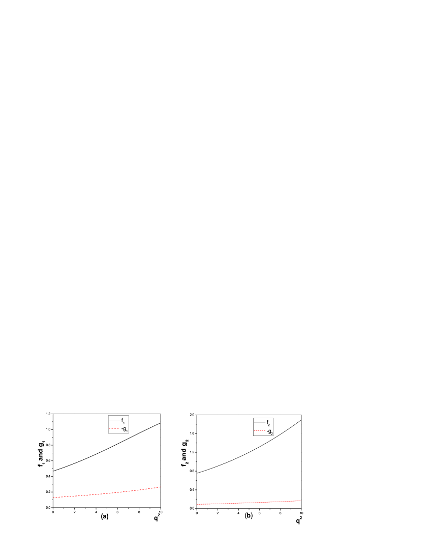
Figure 2: (a) Form factors $f_{1}$ and $g_{1}$     (b) Form factors $f_{2}$ and $g_{2}$

The values shown in Table 2 and Fig. 2 indicate that the form factor $g_{1}$ and $g_{2}$ are small compared with $f_{1}$ and $f_{2}$ and $f_{1}(f_{2})$ and $g_{1}(g_{2})$ have opposite signs, this is similar to the case of $\Theta_{b}\rightarrow\Theta_{c}$ pentaquark2 .

Now let us turn to re-calculate the transition amplitude in the HQET. In the heavy quark limit, we choose $\beta^{\infty}=0.50$ GeV for $\Sigma_{b}$ and $\Sigma_{c}$. The Isgur-Wise function is parameterized as

$$\xi(\omega)=1-\rho^{2}(\omega-1)+\frac{\sigma^{2}}{2}(\omega-1)^{2}+...,$$ (23)

where $\rho^{2}\equiv-\frac{d\zeta(\omega)}{d\omega}|_{\omega=1}$ is the slope parameter and $\sigma^{2}\equiv\frac{d^{2}\zeta(\omega)}{d\omega^{2}}|_{\omega=1}$ is the curvature of the Isgur-Wise function. Our fitted values are

$$\xi_{1}=1-2.09(\omega-1)+1.84(\omega-1)^{2}$$ (24)

$$\xi_{2}=0.42[1-2.79(\omega-1)+3.09(\omega-1)^{2}].$$ (25)

The Isgur-Wise functions in the whole $\omega$ range is depicted in Fig. 3. One can notice that $\xi_{1}(\omega=1)=1$ holds as required by the normalization of the Isgur-Wise function. Even though, as indicated in literature, $\xi_{2}(\omega=1)$ is unknown, at the large $N_{C}$ limit it is determined to be 1/2Chow:1994ni and other early model-dependent studies also confirm this predictionCheng:1996cs .

It is worth indicating clearly that under the heavy quark limit, i.e. $M_{Q}\to\infty$, the mass of heavy quark disappears in the wavefunction (20), but the light constituent mass (anti-quark for meson case and diquark for baryon case) remains. Therefore the theoretical evaluation on the transition rate weakly depends on the light constituent mass even under the heavy quark limit.

From Fig. 3, we observe that $\xi_{2}|_{\omega=1}=0.42$ which is slightly lower than $1/2$. This deviation is due to the mass $m_{diquark}$ in the assumed wavefunction (see Eq.(21)). To further explore the dependence, we deliberately vary $m_{{[ud]}_{V}}$, $\beta_{b[ud]}$ and $\beta_{c[ud]}$. We find that $\xi_{1}$ does not change at all, but the intercept $\xi_{2}(\omega=1)$ changes for different values of $m_{{[ud]}_{V}}$, $\beta_{b[ud]}$ and $\beta_{c[ud]}$. For example, as $\xi_{1}=1$ and $\xi_{2}=0.47$ when one sets $m_{{[ud]}_{V}}=0.5$ GeV, $\beta_{b[ud]}=0.4$ and $\beta_{c[ud]}=0.35$. Definitely non-zero $m_{diquark}$ breaks the heavy quark symmetry $SU_{f}(2)\otimes SU_{s}(2)$, but the violation is still rather small, so that one can use the simplified expression with only two Isgur-Wise functions to approach the transition matrix elements.

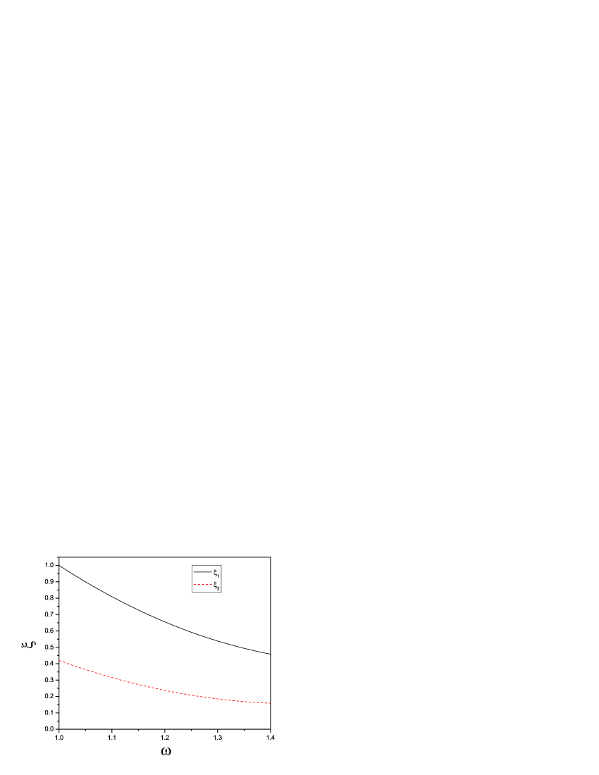
Figure 3: The $\Sigma_{b}\rightarrow\Sigma_{c}$ Isgur-Wise function $\zeta(\omega)$ with diquark mass $m_{{[ud]}_{V}}=770$ MeV.

III.2 Semi-leptonic decay of $\Sigma_{b}\to\Sigma_{c}+l\bar{\nu}_{l}$

With the form factors given in last subsection, we are able to calculate the width of $\Sigma_{b}\to\Sigma_{c}l\bar{\nu}_{l}$.

In table 3 we list our numerical results. The predictions are presented for two cases: with and without taking the heavy quark limit.

It is also interesting to study the longitudinal and transverse helicity amplitudes $H^{V,A}_{\lambda^{\prime},\lambda_{W}}$ where $\lambda^{\prime}$ and $\lambda_{W}$ are the helicities of the daughter baryon and the emitted W-boson respectively, since it may provide more information about the model and even the whole framework. Moreover, several asymmetry parameters $a_{L}$, $a_{T}$ and $P_{L}$ are defined in earlier literature and in this work for readers’ convenience we explicitly present them in the appendix. A ratio of longitudinal to transverse rates $R$ is also defined (see the appendix too), and $R>1$ implies that the longitudinal polarization dominates. Because the values of such asymmetries are more sensitive to the details of the employed models, comparing the theoretical predictions on them with the data which will be available soon at LHC as expected, can help to gain a better understanding of the models.

In Tab.3 the predictions achieved with other approaches Ebert:2006rp are also presented. One notices from Tab.3 that there is an obvious discrepancy between predictions on the semi-leptonic decay widths and $R$ values estimated by different models. The future experimental measurements would provide a chance to test the applicability of different approaches.

Table 3: The widths (in unit $10^{10}{\rm s}^{-1}$) and polarization asymmetries of $\Sigma_{b}\to\Sigma_{c}l\bar{\nu}_{l}$ .

	${\rm width}$	$a_{L}$	$a_{T}$	$\Gamma_{L}$	$\Gamma_{T}$	$R$	$P_{L}$
this work	$1.38$	0.715	-0.893	1.06	0.32	3.25	0.337
this work	$1.60$	0.706	-0.966	1.09	0.51	2.13	0.171
spectator-quark modela Singleton:1990ye	$4.3$	-	-	3.93	0.37	10.7	-
relativistic quark modelbEbert:2006rp	$1.44$	-	-	1.23	0.21	5.89	-
the Bethe-Salpeter approachbIvanov:1998ya	$1.65$	-	-	-	-	-	-
relativistic three-quark modelbIvanov:1996fj	$2.23$	-	-	1.90	0.33	5.76	-

III.3 Non-leptonic decays of $\Sigma_{b}\to\Sigma_{c}+M$

From the theoretical aspects, calculating the concerned quantities of the non-leptonic decays seem to be much more complicated than the semi-leptonic ones. Our theoretical framework is based on the factorization assumption, namely the hadronic transition matrix element is factorized into a product of two independent matrix elements of currents. One of them is determined by a decay constant whereas the other is decomposed into a sum of a few terms according to the Lorentz structure of the current and their coefficients are the to-be-determined form factors. The decays $\Sigma_{b}^{0}\to\Sigma_{c}+M^{-}$ is the so-called color-favored transition, thus and factorization should be a good approximation. Therefore, the study on these non-leptonic decays can be a check of the consistency of the obtained form factors in the heavy bottomed baryon system.

The formulas of the decay rates for non-leptonic decays $\Sigma_{b}\to\Sigma_{c}+M$ in the factorization approach are given in Ref.KK and collected in our previous paper Ke:2007tg . Our numerical results are shown in Tab.4. The CKM matrix elements, the effective Wilson coefficient $a_{1}=1$ and the meson decay constants are the same as in Ref.Ke:2007tg .

4. Two comments are made:

(1) The ratio $\frac{BR(\Sigma_{b}^{0}\to\Sigma_{c}^{+}l^{-}\bar{\nu}_{l})}{BR(\Sigma_{b}^{0}\to\Sigma_{c}^{+}\pi^{-})}$ is $11.4$ which will be experimentally tested.

(2)The up-down asymmetry $\alpha$ for $\Sigma_{b}\to\Sigma_{c}V$ is negative but that for $\Sigma_{b}\to\Sigma_{c}P$ is positive where $\alpha$ is defined in the appendix .

Table 4: widths (in unit $10^{10}{\rm s}^{-1}$) and up-down asymmetries of non-leptonic decays $\Sigma_{b}\to\Sigma_{c}M$ with the light diquark mass $m_{[ud]}=500$ MeV.

	without the heavy quark limit		with the heavy quark limit
	$\rm width$	$\alpha$	$\rm width$	$\alpha$
$\Sigma_{b}^{0}\to\Sigma_{c}^{+}\pi^{-}$	$0.140$	$0.514$	$0.146$	$0.556$
$\Sigma_{b}^{0}\to\Sigma_{c}^{+}\rho^{-}$	$0.166$	$-0.653$	$0.0907$	$-0.785$
$\Sigma_{b}^{0}\to\Sigma_{c}^{+}K^{-}$	$0.0115$	$0.510$	$0.0118$	$0.548$
$\Sigma_{b}^{0}\to\Sigma_{c}^{+}K^{*-}$	$0.00864$	$-0.629$	$0.00471$	$-0.750$
$\Sigma_{b}^{0}\to\Sigma_{c}^{+}a_{1}^{-}$	$0.163$	$-0.551$	$0.0880$	$-0.646$
$\Sigma_{b}^{0}\to\Sigma_{c}^{+}D_{s}^{-}$	$0.796$	$0.379$	$0.655$	$0.425$
$\Sigma_{b}^{0}\to\Sigma_{c}^{+}D^{*-}_{s}$	$0.292$	$-0.302$	$0.152$	$-0.317$
$\Sigma_{b}^{0}\to\Sigma_{c}^{+}D^{-}$	$0.0266$	$0.408$	$0.0242$	$0.440$
$\Sigma_{b}^{0}\to\Sigma_{c}^{+}{D^{*}}^{-}$	$0.0137$	$-0.331$	$0.00694$	$-0.356$

III.4 Estimate on the transition of $\Omega_{b}\to\Omega_{c}$

Though we focus on the transition of $\Sigma_{b}\to\Sigma_{c}$ in this work, the formulas deduced in section II can be applied to calculate the transition between the $\frac{1}{2}^{+}$ baryons such as $\Omega_{b}$ and $\Omega_{c}$ whose structure is analogous to $\Sigma_{b(c)}$ in the quark-diquark picture i.e. the diquark is an axial vector. Since the light diquark is regarded as a spectator, under the SU(3) symmetry of light quarks the predictions on the decay rates of $\Sigma_{b}\to\Sigma_{c}$ hold for $\Omega_{b}\to\Omega_{c}$ approximatively. As $\Omega_{b}$ decays via only weak interaction the branching ratios of $\Omega_{b}\to\Omega_{c}$ should be dominant, so that these decays can be detected more easily. Undoubtedly, since the SU(3) symmetry is slightly broken, different input parameters would bring up minor differences for the numerical results of $\Omega_{b}\to\Omega_{c}$ from $\Sigma_{b}\to\Sigma_{c}$, but the deviation should be relatively small, and the allegation is supported by some theoretical studies which compare the width of $\Omega_{b}\to\Omega_{c}e\nu$ with $\Sigma_{b}\to\Sigma_{c}e\nu$ (Tab. 5).

Table 5: Various theoretical predictions on the rates $\Omega_{b}\to\Omega_{c}e\nu$ and $\Sigma_{b}\to\Sigma_{c}e\nu$ (in unit $10^{10}{\rm s}^{-1}$)

Decay	Ebert:2006rp	Singleton:1990ye	Ivanov:1996fj	Ivanov:1998ya
$\Sigma_{b}\to\Sigma_{c}e\nu$	1.44	4.3	2.23	1.65
$\Omega_{b}\to\Omega_{c}e\nu$	1.29	5.4	1.87	1.81

IV Conclusions and discussions

In this paper, we extensively explore the $\Sigma_{b}\to\Sigma_{c}$ transition in all details and estimate the widths for the semi-leptonic decay and non-leptonic two-body decays of $\Sigma_{b}\to\Sigma_{c}$ as well as several relevant measurable quantities. For the heavy baryons the quark-diquark picture is employed, which reduces the three-body structure into a two-body one.

The matrix elements of the transition $\Sigma_{b}\to\Sigma_{c}$ can be parameterized with a few form factors $f_{i}$ and $g_{i}$ ($i=1,2,3$) according to the Lorentz structures, and we obtain these form factors by calculating the transition $\Sigma_{b}\to\Sigma_{c}$ in the LFQM and evaluate them numerically. The form factors $f_{1}$ and $f_{2}$ for $\Sigma_{b}\to\Sigma_{c}$ are much larger than $g_{1}$ and $g_{2}$, it is noted that $f_{1}(f_{2})$ and $g_{1}(g_{2})$ have opposite signs. Furthermore, we also derive the generalized Isgur-Wise functions $\xi_{1}$ and $\xi_{2}$ under the heavy quark limit. We find that $\xi_{1}(\omega=1)=1$ is consistent with the normalization condition, but $\xi_{2}(\omega=1)$ is slightly lower than 1/2 which was predicted by large $N_{c}$ theory. Our analysis indicates that the deviation is due to the non-zero mass of the light constituents in hadrons (meson and baryon). With the form factors derived in terms of the LFQM or the Isgur-Wise functions we evaluate the semi-leptonic decay rates of $\Sigma_{b}\to\Sigma_{c}$ with and without taking the heavy quark limit. The results with and without heavy quark limit do not decline much from each other, moreover, our numerical results of the rates are generally consistent with that estimated by different approaches. However, it is interesting to note that for the transverse polarization asymmetry $P_{L}$, there is an obvious discrepancy between our results and those by other approaches. Moreover, in terms of SU(3) symmetry of light quarks we estimate the rates $\Omega_{b}\to\Omega_{c}$ which is approximately equal to those of $\Sigma_{b}\to\Sigma_{c}$.

Since the LHCb is running successfully and a remarkable amount of data on $\Sigma_{b}$ and $\Omega_{b}$ production and decay is being accumulated, especially by the LHCb detector, thus we have all confidence that in near future (maybe not next year, but anyhow won’t be too far away), their decay rates and even the asymmetries would be more accurately measured, and we will have a great opportunity to testify our models.

Now let us estimate the feasibility of observing the decay process $\Sigma_{b}\rightarrow\Sigma_{c}l\nu_{l}$. Firstly, we use the code PYTHIA8.1 to calculate the production cross section of $\Sigma_{b}^{+}$ via $pp\rightarrow b\bar{b}\rightarrow\Sigma_{b}^{+}+X$. By the PYTHIA8.1Bargiotti:2007zz ; Brambilla:2010cs ; Sjostrand:2007gs , 100000 $b\bar{b}$ pairs are generated at the $E_{\mathrm{CM}}=7\mathrm{TeV}$. Then $N_{\Sigma_{b}^{+}}=354$ are produced and the corresponding production cross section is $\sigma_{\Sigma_{b}^{+}}\approx 354/100000=3.54\times 10^{-3}\sigma_{b\bar{b}}$. In 2011, the integrated luminosity of the LHCb is $1\;fb^{-1}$Rodrigues:2011zz and the production cross section of the $b\bar{b}$ pairs is $\sigma_{b\bar{b}}=288\mu b$Aaij:2011jh , so our estimate is that about $1.02\times 10^{9}$ $\Sigma_{b}^{+}$ exist in the 2011 data.

Because the LHCb detector is good at tracking the charged particles, such as $p^{+}$, $K^{\pm}$ and $\pi^{\pm}$ and charged leptons, we suggest the decay chain used to find the $\Sigma_{b}$’s semileptonic decay is that: $\Sigma_{b}^{+}\rightarrow\Sigma_{c}^{0}\mu^{+}\nu_{\mu}$, $\Sigma_{c}^{0}\rightarrow\Lambda_{c}^{+}\pi^{-}$ (the branching ratio is $\Gamma_{\Lambda_{c}^{+}\pi^{-}}/\Gamma_{\Sigma_{c}}\approx 100\%$) and $\Lambda_{c}^{+}\rightarrow pK^{+}\pi^{-}$ (the branching ratio is $\Gamma_{pK^{+}\pi^{-}}/\Gamma_{\Lambda_{c}}\approx 5\%$). So, the measurable number of this decay chain is:

$$\mathcal{N}_{\Sigma_{b}}=1.02\times 10^{9}\times{\Gamma_{\Sigma_{c}\mu\nu_{\mu}}\over\Gamma_{\Sigma_{b}}}\times 100\%\times 5\%\times\epsilon_{\mathrm{trig}}\times\epsilon_{\theta},$$ (26)

where, ${\Gamma_{\Sigma_{c}\mu\nu_{\mu}}/\Gamma_{\Sigma_{b}}}$ stands for the branching ratio of $\Sigma_{b}$’s semi-leptonic decay, the $\epsilon_{\mathrm{trig}}$ is the efficiency of the detection trigger and $\epsilon_{\theta}\approx 20\%$ is the efficiency of the detector’s geometric acceptanceHe:2010zqa . Without losing generality, we set $\epsilon_{\mathrm{trig}}=88\%$ here (also given in He:2010zqa ). The decay width of $\Sigma_{b}$ is not known yet. Since QCD is flavor-blind, thus we have reason to believe that considering the phase space of final state the decay width of the $\Sigma_{b}$ should be related to that of $\Gamma_{\Lambda_{b}}$, $\Gamma_{\Lambda_{c}}$ and $\Gamma_{\Sigma_{c}}$ as:

$$\Gamma_{\Sigma_{b}}=\Gamma_{\Lambda_{b}}{\Gamma_{\Sigma_{c}}\over\Gamma_{\Lambda_{c}}}=4.81\times 10^{10}({\,\rm in\,unit}10^{10}s^{-1}).$$ (27)

Substituting all these values back into Eq.(26) ( $\Gamma_{\Sigma_{c}\mu\nu_{\mu}}=1.38\times 10^{10}s^{-1}$ can be found in Tab-3), we have the number of signals of $\Sigma_{b}\to\Sigma_{c}+l\bar{\nu}$:

$$\mathcal{N}_{\Sigma_{b}}=1.87\times 10^{-4}\frac{\Gamma_{\Sigma_{c}\mu\nu_{\mu}}}{10^{10}s^{-1}}=2.58\times 10^{-4}.$$ (28)

If the luminosity of LHCb is not increased greatly in the future to avoid the high level pile-up, we conclude that, since the strong decay $\Sigma_{b}\rightarrow\Lambda_{b}\pi$ dominates and the lifetime of $\Sigma_{b}$ is determined by the mode, the branching ratio of the weak decay is significantly suppressed, it would be hard to directly observe the signals of semileptonic decays of $\Sigma_{b}$. Since the signal of the semileptonic decays of $\Sigma_{b}$ is clear and related to new physics, so that is worth careful investigation at LHCb, even though it is almost impossible to be measured for the present luminosity if only SM applies. Thus, as analyzed above, we would recommend to measure $\Omega_{b}\to\Omega_{c}$ transitions because $\Omega_{b}$ does not decay via strong interaction, so $\Omega_{b}\to\Omega_{c}+l\bar{\nu}$ and $\Omega_{b}\to\Omega_{c}+M$ would be the dominant modes. It enables us to make a more precise measurement by which we can not only further investigate the validity of the diquark picture for heavy baryons, but also create an opportunity to search for new physics beyond the SM, at least check if the new physics scenario shows up in such transitions. We also suggest to measure the quantities such as the asymmetries besides the widths, because of the obvious advantages about our models and physics.

Appendix A Semi-leptonic decays of $\Sigma_{b}\to\Sigma_{c}l\bar{\nu}_{l}$

The helicity amplitudes are related to the form factors for $\Sigma_{b}\to\Sigma_{c}$ through the following expressions KKP

$$H^{V}_{\frac{1}{2},0} = \frac{\sqrt{Q_{-}}}{\sqrt{q^{2}}}\left(\left(M_{\Sigma_{b}}+M_{\Sigma_{c}}\right)f_{1}-\frac{q^{2}}{M_{\Sigma_{b}}}f_{2}\right),$$

$$H^{V}_{\frac{1}{2},1} = \sqrt{2Q_{-}}\left(-f_{1}+\frac{M_{\Sigma_{b}}+M_{\Sigma_{c}}}{M_{\Sigma_{b}}}f_{2}\right),$$

$$H^{A}_{\frac{1}{2},0} = \frac{\sqrt{Q_{+}}}{\sqrt{q^{2}}}\left(\left(M_{\Sigma_{b}}-M_{\Sigma_{c}}\right)g_{1}+\frac{q^{2}}{M_{\Sigma_{b}}}g_{2}\right),$$

$$H^{A}_{\frac{1}{2},1} = \sqrt{2Q_{+}}\left(-g_{1}-\frac{M_{\Sigma_{b}}-M_{\Sigma_{c}}}{M_{\Sigma_{b}}}g_{2}\right).$$ (29)

where $Q_{\pm}=2(P\cdot P^{\prime}\pm M_{\Sigma_{b}}M_{\Sigma_{c}})$. The amplitudes for the negative helicities are obtained in terms of the relation

$$H^{V,A}_{-\lambda^{\prime}-\lambda_{W}}=\pm H^{V,A}_{\lambda^{\prime},\lambda_{W}},$$ (30)

where the upper (lower) sign corresponds to V(A). The helicity amplitudes are

$$H_{\lambda^{\prime},\lambda_{W}}=H^{V}_{\lambda^{\prime},\lambda_{W}}-H^{A}_{\lambda^{\prime},\lambda_{W}}.$$ (31)

The helicities of the $W$-boson $\lambda_{W}$ can be either $0$ or $1$, which correspond to the longitudinal and transverse polarizations, respectively. The longitudinally (L) and transversely (T) polarized rates are respectivelyKKP

$$\frac{d\Gamma_{L}}{d\omega} = \frac{G_{F}^{2}|V_{cb}|^{2}}{(2\pi)^{3}}~{}\frac{q^{2}~{}p_{c}~{}M_{\Sigma_{c}}}{12M_{\Sigma_{b}}}\left[|H_{\frac{1}{2},0}|^{2}+|H_{-\frac{1}{2},0}|^{2}\right],$$

$$\frac{d\Gamma_{T}}{d\omega} = \frac{G_{F}^{2}|V_{cb}|^{2}}{(2\pi)^{3}}~{}\frac{q^{2}~{}p_{c}~{}M_{\Sigma_{c}}}{12M_{\Sigma_{b}}}\left[|H_{\frac{1}{2},1}|^{2}+|H_{-\frac{1}{2},-1}|^{2}\right].$$ (32)

where $p_{c}$ is the momentum of $\Sigma_{c}$ in the reset frame of $\Sigma_{b}$.

The integrated longitudinal and transverse asymmetries defined as

$$a_{L} = \frac{\int_{1}^{\omega_{\rm max}}d\omega~{}q^{2}~{}p_{c}\left[|H_{\frac{1}{2},0}|^{2}-|H_{-\frac{1}{2},0}|^{2}\right]}{\int_{1}^{\omega_{\rm max}}d\omega~{}q^{2}~{}p_{c}\left[|H_{\frac{1}{2},0}|^{2}+|H_{-\frac{1}{2},0}|^{2}\right]},$$

$$a_{T} = \frac{\int_{1}^{\omega_{\rm max}}d\omega~{}q^{2}~{}p_{c}\left[|H_{\frac{1}{2},1}|^{2}-|H_{-\frac{1}{2},-1}|^{2}\right]}{\int_{1}^{\omega_{\rm max}}d\omega~{}q^{2}~{}p_{c}\left[|H_{\frac{1}{2},1}|^{2}+|H_{-\frac{1}{2},-1}|^{2}\right]}.$$ (33)

The ratio of the longitudinal to transverse decay rates $R$ is defined by

$$R=\frac{\Gamma_{L}}{\Gamma_{T}}=\frac{\int_{1}^{\omega_{\rm max}}d\omega~{}q^{2}~{}p_{c}\left[|H_{\frac{1}{2},0}|^{2}+|H_{-\frac{1}{2},0}|^{2}\right]}{\int_{1}^{\omega_{\rm max}}d\omega~{}q^{2}~{}p_{c}\left[|H_{\frac{1}{2},1}|^{2}+|H_{-\frac{1}{2},-1}|^{2}\right]},$$ (34)

and the longitudinal $\Sigma_{c}$ polarization asymmetry $P_{L}$ is given as

$$P_{L} = \frac{\int_{1}^{\omega_{\rm max}}d\omega~{}q^{2}~{}p_{c}\left[|H_{\frac{1}{2},0}|^{2}-|H_{-\frac{1}{2},0}|^{2}+|H_{\frac{1}{2},1}|^{2}-|H_{-\frac{1}{2},-1}|^{2}\right]}{\int_{1}^{\omega_{\rm max}}d\omega~{}q^{2}~{}p_{c}\left[|H_{\frac{1}{2},0}|^{2}+|H_{-\frac{1}{2},0}|^{2}+|H_{\frac{1}{2},1}|^{2}+|H_{-\frac{1}{2},-1}|^{2}\right]}.$$ (35)

References

• (1) H. W. Ke, X. Q. Li and Z. T. Wei, Phys. Rev.  D 77, 014020 (2008) [arXiv:0710.1927 [hep-ph]].
• (2) H. Park et al. [HyperCP Collaboration], Phys. Rev. Lett.  94, 021801 (2005) [arXiv:hep-ex/0501014].
• (3) X. G. He, J. Tandean and G. Valencia, Phys. Rev. Lett.  98, 081802 (2007) [arXiv:hep-ph/0610362].
• (4) X. G. He, J. Tandean and G. Valencia, Phys. Lett.  B 631, 100 (2005) [arXiv:hep-ph/0509041].
• (5) N. Isgur and M. Wise, Nucl. Phys. B 348, 276 (1991); H. Georgi, Nucl. Phys. B 348, 293 (1991).
• (6) J. G. Korner and P. Kroll, Z. Phys.  C 57, 383 (1993).
• (7) D. Ebert, R. N. Faustov and V. O. Galkin, Phys. Rev.  D 73, 094002 (2006) [arXiv:hep-ph/0604017].
• (8) R. L. Singleton, Phys. Rev.  D 43, 2939 (1991).
• (9) M. A. Ivanov, V. E. Lyubovitskij, J. G. Korner and P. Kroll, Phys. Rev.  D 56, 348 (1997) [arXiv:hep-ph/9612463].
• (10) M. A. Ivanov, J. G. Korner, V. E. Lyubovitskij and A. G. Rusetsky, Phys. Rev.  D 59, 074016 (1999) [arXiv:hep-ph/9809254].
• (11) F. Wilczek, arXiv: hep-ph/0409168.
• (12) P. Guo, H. Ke, X. Li, C. Lu and Y. Wang, Phys. Rev. D 75, 054017 (2007).
• (13) Y. Yu, H. Ke, Y. Ding, X. Guo, H. Jin, X. Li, P. Shen and G. Wang, Commun. Theor. Phys. 46, 1031 (2006); Y. Yu, H. Ke, Y. Ding, X. Guo, H. Jin, X. Li, P. Shen and G. Wang, arXiv: hep-ph/0611160.
• (14) Z. T. Wei, H. W. Ke and X. Q. Li, Phys. Rev.  D 80, 094016 (2009) [arXiv:0909.0100 [hep-ph]].
• (15) Y. Dai, X. Guo and C. Huang, Nucl.Phys. B412 (1994) 277.
• (16) W. Jaus, Phys. Rev. D 41, 3394 (1990); D 44, 2851 (1991); W. Jaus, Phys. Rev.  D 60, 054026 (1999).
• (17) C. R. Ji, P. L. Chung and S. R. Cotanch, Phys. Rev.  D 45, 4214 (1992).
• (18) H. Y. Cheng, C. Y. Cheung and C. W. Hwang, Phys. Rev.  D 55, 1559 (1997) [arXiv:hep-ph/9607332].
• (19) H. Y. Cheng, C. K. Chua and C. W. Hwang, Phys. Rev.  D 69, 074025 (2004).
• (20) C. W. Hwang and Z. T. Wei, J. Phys. G 34, 687 (2007); C. D. Lu, W. Wang and Z. T. Wei, Phys. Rev.  D 76, 014013 (2007) [arXiv:hep-ph/0701265].
• (21) H. M. Choi, Phys. Rev.  D 75, 073016 (2007) [arXiv:hep-ph/0701263];
• (22) H. W. Ke, X. Q. Li and Z. T. Wei, Phys. Rev.  D 80, 074030 (2009) [arXiv:0907.5465 [hep-ph]]; H. W. Ke, X. Q. Li, Z. T. Wei and X. Liu, Phys. Rev.  D 82, 034023 (2010) [arXiv:1006.1091 [hep-ph]].
• (23) G. Li, F. l. Shao and W. Wang, Phys. Rev.  D 82, 094031 (2010) [arXiv:1008.3696 [hep-ph]].
• (24) Z. T. Wei, H. W. Ke and X. F. Yang, Phys. Rev.  D 80, 015022 (2009) [arXiv:0905.3069 [hep-ph]]; H. W. Ke, X. Q. Li and Z. T. Wei, Eur. Phys. J.  C 69, 133 (2010) [arXiv:0912.4094 [hep-ph]]; H. W. Ke, X. H. Yuan and X. Q. Li, Int. J. Mod. Phys. A 26, 4731 (2010), arXiv:1101.3407 [hep-ph]. H. W. Ke and X. Q. Li, Eur. Phys. J.  C 71, 1776 (2011) [arXiv:1104.3996 [hep-ph]]; H. W. Ke and X. Q. Li, Phys. Rev.  D 84, 114026 (2011) [arXiv:1107.0443 [hep-ph]]; H. W. Ke and X. Q. Li, Eur. Phys. J.  C 71, 1776 (2011) [arXiv:1104.3996 [hep-ph]].
• (25) H. Cheng and C. Chua , Phys. Rev. D 70, 034007 (2004).
• (26) For a review, see M. Neubert, Phys. Rept. 245, 259 (1994).
• (27) K. Nakamura et al. [Particle Data Group], J. Phys. G 37, 075021 (2010).
• (28) B. Ram and V. Kriss, Phys. Rev.  D 35, 400 (1987).
• (29) C. K. Chow, Phys. Rev.  D 51, 1224 (1995) [arXiv:hep-ph/9408364].
• (30) H. Y. Cheng, Phys. Rev.  D 56, 2799 (1997) [arXiv:hep-ph/9612223].
• (31) J. K$\rm{\ddot{o}}$rner and M. Kr$\rm\ddot{a}$mer, Z. Phys. C 55, 659 (1992).
• (32) M. Bargiotti and V. Vagnoni, CERN-LHCB-2007-042.
• (33) N. Brambilla et al., Eur. Phys. J.  C 71, 1534 (2011) [arXiv:1010.5827 [hep-ph]].
• (34) T. Sjostrand, S. Mrenna and P. Z. Skands, Comput. Phys. Commun.  178, 852 (2008) [arXiv:0710.3820 [hep-ph]].
• (35) E. Rodrigues [LHCb Collaboration], J. Phys. Conf. Ser.  335, 012034 (2011).
• (36) R. Aaij et al. [LHCb Collaboration], Eur. Phys. J. C 71, 1645 (2011) [arXiv:1103.0423 [hep-ex]].
• (37) J. He and F. t. L. collaboration, arXiv:1001.5370 [hep-ex].
• (38) J. K$\rm\ddot{o}$rner and M. Kr$\rm\ddot{a}$mer, Phys. Lett. B 275, 495 (1992); P. Bialas, J. K$\rm\ddot{o}$rner, M. Kr$\rm\ddot{a}$mer, and K. Zalewski, Z. Phys. C 57, 115 (1993); J. K$\rm{\ddot{o}}$rner, M. Kr$\rm\ddot{a}$mer and D. Pirjol, Prog. Part. Nucl. Phys. 33, 787 (1994).