Ward Identity Implies Recursion Relation at Tree and Loop Level

Abstract

In this article, we use Ward identity to calculate tree and one loop level off shell amplitudes in pure Yang-Mills theory with a pair of external lines complexified. We explicitly prove Ward identity at tree and one loop level using Feynman rules, and then give recursion relations for the off shell amplitudes. We find that the cancellation details in the proof of Ward identity simplifies our derivation of the recursion relations. Then we calculate three and four point one loop off shell amplitudes as examples of our method.

I Introduction

At tree level, the amplitudes of pure Yang-Mills fields can be written as rational functions of external momenta and polarization vectors in spinor form Parke:1986gb ; Xu:1986xb ; Berends:1987me ; Kosower ; Dixon1 ; Witten1 . Such rational functions can be analyzed in detail in algebra system. According to this, BCFW recursion relation was proposed and developed in Britto:2004nj ; Britto:2004nc ; Britto:2004ap , and then proved in Britto:2005fq using the pole structure of the tree level on shell amplitudes. This has been an exiting progress on the amplitudes in pure Yang-Mills theory. For theory with massive fields Badger1 ; Ozeren ; Schwinn ; Chen1 ; Chen2 , the amplitudes are also rational functions of external momenta and polarization vectors in spinor form.

At loop level, although the whole amplitudes are no longer rational functions in general, they can be decomposed into some basic scalar integrals with coefficients being rational functions of external spinors BernD1 ; BernD2 . The coefficient structures are studied in depth in Dixon4 ; Bern ; Bern1 . On the other hand, the integrands of the amplitudes are rational functions of the external spinors and integral momenta. For the N=4 planar super Yang-Mills theory, Nima gives an explicit recursive formula for the all-loop integrand of scattering amplitudes.

The amplitudes in gauge theory are constrained by gauge symmetry. This leads to Ward identity which constrains the amplitudes at all loop level. Inspired by the BCFW momenta shift, we considered the Ward identity for tree level amplitudes with complexified momenta for a pair of external lines, and then obtained a recursion relation for the boundary terms using BCFW technique in our recent article Chen . However, in Chen , we chose a particular momenta shift such that the external states of the complexified lines are independent of the complex parameter $z$. Then a natural question is how to obtain a recursion relation for other possible momenta shifts. Furthermore, is it possible to obtain the full amplitudes from the Ward identity, and to extend the technique to one loop amplitudes? In this article, we will give positive answers to all these questions.

In section II, we first give the proof of Ward identity at tree level using Feynman rules directly, and then derive the recursion relation for off shell amplitudes, where the cancellation details in the proof of Ward identity helps to simplify the recursion relations. Section III is parallel to section II. We first extend the proof of Ward identity to one loop level and then derive the recursion relation for one loop off shell amplitudes. Our technique does not rely on the on-shell momenta shifts. Also, in our calculation using the recursion relation, four point vertexes are not used explicitly. We calculate three and four point one loop off shell amplitudes as examples in section III.3.

II Ward Identity and Implied Recursion Relation at Tree Level

In Chen , we directly proved complexified Ward identity for pure Yang-Mills fields at tree level, and then used it to deduce a recursion relation for the boundary terms of the complexified amplitudes. Here we generalize the method to deduce a recursion relation for tree level amplitudes with one external off shell line. This section will serve as a basis for our generalization to one loop level in the next section. We will call the external off shell line $L_{\mbox{\tiny off}}$ with momentum $k_{\mbox{\tiny off}}^{\mu}$, and the corresponding off shell amplitudes $A_{\mu}$.

II.1 Proof of Ward Identity at Tree Level

Although done in our previous paper Chen , we briefly summerize some key points in the direct proof of tree level Ward identity, since these points are useful for deriving tree level recursion relation and also will be part of the proof at one loop level in the next section.

The amplitude is complexified by shifting the momenta of a pair of external lines. We choose $L_{\mbox{\tiny off}}$ and one on shell line $L_{s}$ with momentum $k_{s}=\lambda_{s}\tilde{\lambda}_{s}$, and the shift is:

$$k_{s}\rightarrow k_{s}-z\eta,\ \ \ \ \ \ \ \ \ \ \ \ \ \ k_{\mbox{\tiny off}}\rightarrow k_{\mbox{\tiny off}}+z\eta,$$ (1)

where z is the complexifing parameter and $\eta$ should satisfy $\eta^{2}=0$ and $k_{s}\cdot\eta=0$.

The color ordered Feynman rules of the gauge field are as in Dixon1 , with outgoing momenta. We also write the Feynman rules for ghost fields here in Figure 1, which will be used in the next section.

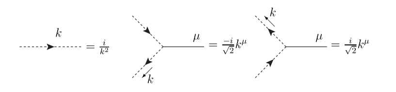
Figure 1: Ghost field color ordered Feynman rules. Dashed line for ghost field and solid line for gauge field.

For a three point vertex with line 1, 2 and $L_{\mbox{\tiny off}}$ in anti-clockwise order, we write it in the following form:

$$V_{\mu_{1}\mu_{2}\mu} \equiv S_{\mu_{1}\mu_{2}\mu}+R_{\mu_{1}\mu_{2}\mu}+M_{\mu_{1}\mu_{2}\mu},$$ (2)

where

$$S_{\mu_{1}\mu_{2}\mu} = \frac{i}{\sqrt{2}}\left(\eta_{\mu_{1}\mu_{2}}(k_{1}-k_{2})_{\mu}\right)$$

$$R_{\mu_{1}\mu_{2}\mu} = \frac{i}{\sqrt{2}}\left(-2\eta_{\mu_{2}\mu}(k_{\mbox{\tiny off}})_{\mu_{1}}+2\eta_{\mu\mu_{1}}(k_{\mbox{\tiny off}})_{\mu_{2}}\right)$$

$$M_{\mu_{1}\mu_{2}\mu} = \frac{i}{\sqrt{2}}\left(-\eta_{\mu_{2}\mu}(k_{1})_{\mu_{1}}+\eta_{\mu\mu_{1}}(k_{2})_{\mu_{2}}\right).$$ (3)

We will refer to these terms as S, R and M parts of the vertex. Contracting this vertex with $k_{\mbox{\tiny off}}$, we get:

$$k_{\mbox{\tiny off}}^{\mu}\cdot V_{\mu_{1}\mu_{2}\mu}=\frac{i}{\sqrt{2}}\eta_{\mu_{1}\mu_{2}}k_{2}^{2}-\frac{i}{\sqrt{2}}\eta_{\mu_{1}\mu_{2}}k_{1}^{2}+\frac{i}{\sqrt{2}}k_{2\ \mu_{2}}k_{3}{}_{\ \mu_{1}}-\frac{i}{\sqrt{2}}k_{1\ \mu_{1}}k_{3}{}_{\ \mu_{2}},$$ (4)

and we represent these terms by the symbols in Figure 2. These terms are frequently used throughout the paper, and we will call the terms in the first line of Figure 2 as solid triangle terms, and the second line terms as hollow triangle terms.

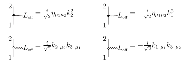
Figure 2: Notations for 4. We specialize $L_{\mbox{\tiny off}}$ using photon line.

Then a proof of tree level Ward identity can be shown in several steps. Assume it holds for N-point and less than N-point amplitudes(for example, 3-point case can be immediately checked), we will show how it holds for (N+1) point amplitudes. We choose $L_{\mbox{\tiny off}}$ as the (N+1)-th line. We can construct an (N+1)-point color ordered diagram from an N-point one by inserting $L_{\mbox{\tiny off}}$ to an N-point diagram between Line 1 and Line N.

First, when $L_{\mbox{\tiny off}}$ is inserted to a propagator or Line 1 or Line N, we denote the vertex as $V_{\mbox{\tiny off}}$, and contract it with $k_{\mbox{\tiny off}}$, the following two hollow triangle terms in Figure 3 vanish due to less-point Ward Identities or the on-shell conditions of Line 1 or N. The meaning of the symbols are in Figure 2.

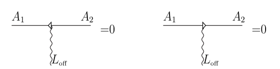
Figure 3: When $L_{\mbox{\tiny off}}$ is inserted to a propagator or Line 1 or Line N, these terms vanish due to less point Ward identity or the on-shell conditions of Line 1 or N. $A_{1}$ and $A_{2}$ are sub amplitudes.

Second, $L_{\mbox{\tiny off}}$ is inserted to a three-point vertex in the N-point diagram. These terms and the remaining terms, ie. solid triangle terms, from the above case can be re-combined as in Figure 4 to cancel each other.

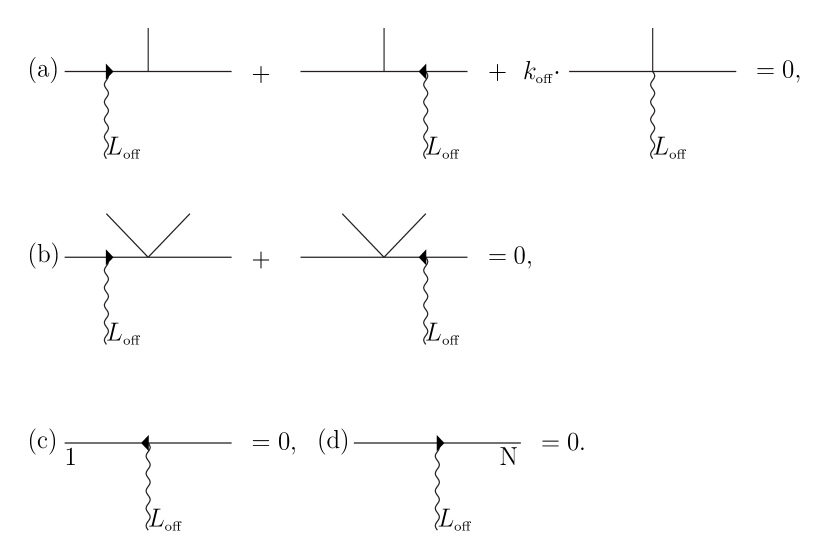
Figure 4: A group of diagrams cancel. In (a) and (b), the cancellation is solely due to the vertex structures, not dependent on whether the legs are on shell or off shell. (c) and (d) are due to on shell conditions for Line 1 and Line N: $k_{1}^{2}=0$ and $k_{N}^{2}$=0.

Figure 3 and Figure 4 constitute the proof of Ward identity at tree level.

II.2 Recursion Relation for Tree Level Off Shell Amplitudes

As discussed in Chen , from the complexified Ward identity ${{\hat{k}}_{\mbox{\tiny off}}}^{\mu}\cdot{\hat{A}}_{\mu}=0$, by a derivative over z we get:

$$\hat{A}_{\mu}\eta^{\mu}|_{z\rightarrow 0}=-{d\hat{A}_{\mu}\over dz}{\hat{k}}_{\mbox{\tiny off}}^{\mu}|_{z\rightarrow 0}.$$ (5)

The symbol $\hat{}$ represents that the quantity is complexified, ie. depends on the shift parameter z. Here $k_{\mbox{\tiny off}}$ is shifted as in 1: ${\hat{k}}_{\mbox{\tiny off}}=k_{\mbox{\tiny off}}+z\eta$. Our destination is to calculate $A_{\mu}$, and we will realize it by calculating the right hand side of 5.

We name the vertex which contains $L_{\mbox{\tiny off}}$ as $V_{\mbox{\tiny off}}$. At tree level, we have the following three cases:

1. the derivative acts on a propagator;

2. the derivative acts on a three point vertex which does not contain $L_{\mbox{\tiny off}}$;

3. the derivative acts on a three point vertex $V_{\mbox{\tiny off}}$.

In the first and second cases, when $V_{\mbox{\tiny off}}$ is a three point vertex, we write $k_{\mbox{\tiny off}}^{\mu}\cdot V_{\mbox{\tiny off}}{}_{\ \mu}$ as in Figure 2, and take out the hollow triangle terms. These terms, together with the terms from the third case where the derivative acts on the M part of $V_{\mbox{\tiny off}}{}_{\ \mu}$ as written in II.1, add up to be 0 due to Ward identity for some sub amplitudes.

From above we know that in the first and second cases, we only need the solid triangle terms for $k_{\mbox{\tiny off}}^{\mu}\cdot V_{\mbox{\tiny off}}{}_{\ \mu}$ as represented in Figure 2, when $V_{\mbox{\tiny off}}$ is a three point vertex; in the third case, $\frac{d}{dz}$ only need to act on the S and R part of $V_{\mbox{\tiny off}}{}_{\ \mu}$ as written in II.1. The first two cases can be further simplified. Due to (a) and (b) in Figure 4, the terms relevant for the first two cases are reduced to those with $k_{\mbox{\tiny off}}$ neighboring to the three point vertex or the propagator to be differentiated, as depicted in Figure 5.

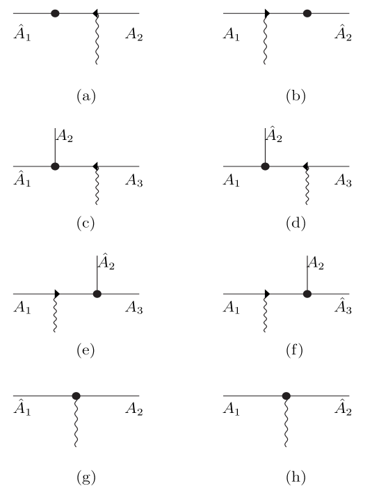
Figure 5: Terms to be calculated for tree-level off-shell amplitudes. Here and following, the dark solid circle symbol $\bullet$ denotes where we act $d\over dz$. We shift $L_{\mbox{\tiny off}}$ and some other line $L_{s}$. $\{A_{i}\}$ denote some sub-diagrams with less external states. $\hat{A}_{k}$ includes $L_{s}$. In different diagrams, the same $A_{k}$ symbols do not mean the same sub amplitudes. They sum over all allowed sub amplitudes.

Thus, for the first case, the diagrams are (a) and (b) in Figure 5. The contributions from (a) and (b) to $-{d\hat{A}_{\mu}\over dz}{\hat{k}}_{\mbox{\tiny off}}^{\mu}|_{z\rightarrow 0}$ are:

$$\mbox{for (a)}\ \ \frac{-i\sqrt{2}}{k_{A_{1}}^{2}k_{A_{2}}^{2}}k_{A_{1}}\cdot\eta\ A_{1}\cdot A_{2},$$

$$\mbox{for (b)}\ \ \frac{i\sqrt{2}}{k_{A_{1}}^{2}k_{A_{2}}^{2}}k_{A_{2}}\cdot\eta\ A_{1}\cdot A_{2}.$$ (6)

As noted in Figure 5, {$A_{i}$} are some less point amplitudes. $k_{A_{i}}$ is the total momentum of the external legs contained in the sub amplitude $A_{i}$. If some $A_{i}$ just contains one external line $L_{m}$, we define this $A_{i}$ to be $ik_{m}^{2}\epsilon_{m}$, and accompany it with a propagator $\frac{-i}{k_{A_{i}}^{2}}=\frac{-i}{k_{m}^{2}}$. Another point is that, although $k_{s}\cdot\eta=0$, we keep it in the evaluations here and below as if it is not 0, as will be explained at the end of this subsection.

The second case corresponds to (c) (d) (e) and (f) in Figure 5, and the contributions to $-{d\hat{A}_{\mu}\over dz}{\hat{k}}_{\mbox{\tiny off}}^{\mu}|_{z\rightarrow 0}$ are:

$$\mbox{for (c)}\ \ \frac{1}{2k_{A_{1}}^{2}k_{A_{2}}^{2}k_{A_{3}}^{2}}(A_{3}\cdot\eta\ A_{1}\cdot A_{2}+A_{1}\cdot\eta\ A_{2}\cdot A_{3}-2A_{2}\cdot\eta\ A_{1}\cdot A_{3}),$$

$$\mbox{for (d)}\ \ \frac{1}{2k_{A_{1}}^{2}k_{A_{2}}^{2}k_{A_{3}}^{2}}(-A_{3}\cdot\eta\ A_{1}\cdot A_{2}+2A_{1}\cdot\eta\ A_{2}\cdot A_{3}-A_{2}\cdot\eta\ A_{1}\cdot A_{3}),$$

$$\mbox{for (e)}\ \ \frac{-1}{2k_{A_{1}}^{2}k_{A_{2}}^{2}k_{A_{3}}^{2}}(-2A_{3}\cdot\eta\ A_{1}\cdot A_{2}+A_{1}\cdot\eta\ A_{2}\cdot A_{3}+A_{2}\cdot\eta\ A_{1}\cdot A_{3}),$$

$$\mbox{for (f)}\ \ \frac{-1}{2k_{A_{1}}^{2}k_{A_{2}}^{2}k_{A_{3}}^{2}}(-A_{1}\cdot\eta\ A_{2}\cdot A_{3}+2A_{2}\cdot\eta\ A_{1}\cdot A_{3}-A_{3}\cdot\eta\ A_{1}\cdot A_{2}).$$ (7)

And the third case corresponds to (g) and (h) in Figure 5, whose contributions are:

$$\mbox{for (g)}\ \ \frac{-i}{\sqrt{2}k_{A_{1}}^{2}k_{A_{2}}^{2}}(k_{\mbox{\tiny off}}\cdot\eta\ A_{1}\cdot A_{2}+2A_{1}\cdot\eta\ k_{\mbox{\tiny off}}\cdot A_{2}-2A_{2}\cdot\eta\ k_{\mbox{\tiny off}}\cdot A_{1}),$$

$$\mbox{for (h)}\ \ \frac{-i}{\sqrt{2}k_{A_{1}}^{2}k_{A_{2}}^{2}}(-k_{\mbox{\tiny off}}\cdot\eta\ A_{1}\cdot A_{2}+2A_{1}\cdot\eta\ k_{\mbox{\tiny off}}\cdot A_{2}-2A_{2}\cdot\eta\ k_{\mbox{\tiny off}}\cdot A_{1}).$$ (8)

As explained before 6, in this case $\frac{d}{dz}$ only need to act on the S and R part of $V_{\mbox{\tiny off}}{}_{\ \mu}$ as written in II.1.

It can be observed that, 7 for $L_{s}$ contained in $A_{1}$ or $A_{2}$ or $A_{3}$, the expressions are the same. In the case when $L_{s}$ is contained in $A_{2}$ we should sum (d) and (e) in Figure 5 to see that the expression is the same as when $L_{s}$ is contained in $A_{1}$ or $A_{3}$. The common expression is:

$$\frac{1}{2k_{A_{1}}^{2}k_{A_{2}}^{2}k_{A_{3}}^{2}}(A_{3}\cdot\eta\ A_{1}\cdot A_{2}+A_{1}\cdot\eta\ A_{2}\cdot A_{3}-2A_{2}\cdot\eta\ A_{1}\cdot A_{3}).$$ (9)

6 and 7 summed up also give a common expression, regardless of whether $L_{s}$ is contained in $A_{1}$ or $A_{2}$:

$$\frac{-i}{\sqrt{2}k_{A_{1}}^{2}k_{A_{2}}^{2}}\left(\ (k_{A_{1}}-k_{A_{2}})\cdot\eta\ A_{1}\cdot A_{2}+2A_{1}\cdot\eta\ k_{\mbox{\tiny off}}\cdot A_{2}-2A_{2}\cdot\eta\ k_{\mbox{\tiny off}}\cdot A_{1}\right)$$ (10)

The final tree level result for $A_{\mu}\eta^{\mu}$ is the sum of 9 and 10, which can be written in the form of $\tilde{A}_{\mu}\eta^{\mu}$. In the expressions we should sum over all allowed allocations of the on shell external legs into $\{A_{i}\}$. It is easy to show that the off shell amplitude $A_{\mu}=\tilde{A}_{\mu}$. In four dimensional spacetime, we only need to find 4 independent $\eta_{i}$ such that $A_{\mu}\eta^{\mu}_{i}=\tilde{A}_{\mu}\eta^{\mu}_{i}$. Since in the shift $\eta^{\mu}$ is required to satisfy $k_{s}\cdot\eta=0$ and $\eta^{2}=0$, the three choices of $\eta_{i}$ as $\epsilon_{s}^{+}$, $\epsilon_{s}^{-}$ or $k_{s}$ satisfy $A_{\mu}\eta^{\mu}_{i}=\tilde{A}_{\mu}\eta^{\mu}_{i}$. The remaining choice of $\eta_{i}$ can be chosen as $k_{\mbox{\tiny off}}$. This is not obvious to satisfy $A_{\mu}\eta^{\mu}_{i}=\tilde{A}_{\mu}\eta^{\mu}_{i}$. However, in our calculations we have kept the terms $k_{s}\cdot\eta$ as if it is not 0, and by this trick it comes out that $\tilde{A}_{\mu}k_{\mbox{\tiny off}}^{\mu}=0=A_{\mu}k_{\mbox{\tiny off}}^{\mu}$. In conclusion $A_{\mu}=\tilde{A}_{\mu}$, where $\tilde{A}_{\mu}$ is contained in the sum of 9 and 10 in form of $\tilde{A}_{\mu}\eta^{\mu}$.

Compare to Berends-Giele recursion relation Berends:1987me , it is seen that 9 corresponds to $k_{\mbox{\tiny off}}$ contained in a four point vertex, and 10 is equivalent to the contribution when $k_{\mbox{\tiny off}}$ is contained in a three point vertex. This on one hand supports the correctness of our method, and on the other hand a little undermines the value of our method at tree level. There are also other recursion relations for off shell tree level amplitudes, eg. Feng . Yet we are going to extend our method to one loop level, where the situation is much more complicated and our method is new.

III Ward Identity and Implied Recursion Relation at 1-loop Level

In this section we are going to extend our method to 1-loop level. We will show how complexified Ward identity holds at 1-loop level and then we deduce the corresponding recursive calculation of 1-loop off shell amplitude. Using our method, we will calculate three and four point 1-loop off shell amplitudes as examples. In our calculation we use FDH scheme Bern:1991aq , in which only the loop momentum is continued to dimensionality different from 4.

We first explain some subtleties at loop level. First, after momentum shifting, some lines on the loop carry complex momenta. This brings ambiguities to the meaning of the loop integral and prevents us from translating the loop momentum $l\rightarrow l+k$ or flip it $l\rightarrow-l$. However, according to equation 5, what we need for our technique is the derivative of the integral at the value $z\rightarrow 0$. And it is easy to prove that:

$$\int d^{D}l\frac{d}{dz}f(l^{\mu},{\hat{k}}^{\mu})|_{z\rightarrow 0}=\int d^{D}l\frac{d}{dz}f(-l^{\mu},{\hat{k}}^{\mu})|_{z\rightarrow 0},$$ (11)

$$\int d^{D}l\frac{d}{dz}f(l^{\mu},{\hat{k}}^{\mu})|_{z\rightarrow 0}=\int d^{D}l\frac{d}{dz}f(l^{\mu}+{\hat{k}}^{\prime\mu},{\hat{k}}^{\mu})|_{z\rightarrow 0}.$$ (12)

Thus for our technique, we can translate or flip the loop momentum even when the integrand is complex.

Second, some attention should be paid to color orderings and symmetry factors. At tree level there is only one color ordering contributing to the the primitive part of the color ordered amplitudes. At one loop level, most diagrams also only have one color ordering. However, for gauge field loop diagrams, there are three kinds of diagrams having two color orderings. Those are diagrams with two vertexes on the loop: two three-point vertexes; two four-point vertexes; a three-point vertex and a four-point vertex. For the first and second cases, the contributions from the two color orderings are the same at integrand level. For the third case, the contributions from the two color orderings at integrand level differ by a translation and flip of the loop momentum, and due to 12 the two orderings contribute the same in our method after integration. In a word, these three kinds of diagrams have a factor of 2 from possible color orderings. At the same time, these three kinds of diagrams have symmetry factor $\frac{1}{2}$, just canceling the doubling from color orderings. For ghost loop diagrams, those with two vertexes on the loop also have a doubling from two color orderings, while there is only either clockwise or anti clockwise ghost loop when there are only two vertexes on the ghost loop. We replace the doubling from color orderings by drawing both clockwise and anti-clockwise ghost loop diagrams, which are actually equal when there are only two vertexes on the ghost loop.

Finally, as our convention for the loop momentum for all our loop diagrams, we specify the loop momentum in the following way. For each external leg $L_{i}$, when we want to make a path from it to the loop, there is one definite vertex $V$ on the loop first encountered in the path, then we say the external leg $L_{i}$ is associated with this loop vertex $V$. We find the vertex with which $L_{\mbox{\tiny off}}$ is associated, call it $V_{0}$. Assume all the lines associated with $V_{0}$ in color ordering are $L_{j},L_{j+1},\cdots,L_{N},L_{\mbox{\tiny off}},L_{1},\cdots,L_{i}$, then we assign the momentum of the first loop propagator on the counter clockwise side of $V_{0}$ as $l-k_{1}-\cdots-k_{i}$, with the loop momentum flowing in counter clockwise direction. $l$ is to be integrated. External leg momenta are outgoing.

III.1 Proof of Ward Identity at 1-Loop Level

In this section we use $A^{l}$ for 1-loop amplitudes, and $A^{t}$ for tree level amplitudes.

Two point and three point 1-loop Ward identity is easy to verify directly. Similar to the proof at tree level, we use induction, assume Ward identity holds for N and less than N point one loop amplitudes, and construct an (N+1) point diagram from an N point one by inserting $k_{\mbox{\tiny off}}$ in different places. We denote the vertex with $k_{\mbox{\tiny off}}$ as $V_{\mbox{\tiny off}}$ and when $V_{\mbox{\tiny off}}$ is a three point vertex, we decompose $k_{\mbox{\tiny off}}\cdot V_{\mbox{\tiny off}}$ as in Figure 2.

Case 1. When $k_{\mbox{\tiny off}}$ is linked to a propagator(including gauge field loop propagator) or external line of the N point diagram, the solid triangle terms from $k_{\mbox{\tiny off}}\cdot V_{\mbox{\tiny off}}$ mostly cancel the terms with $k_{\mbox{\tiny off}}$ in a four point vertex, in the manner of Figure 4. Only the terms in Figure 6 remain.

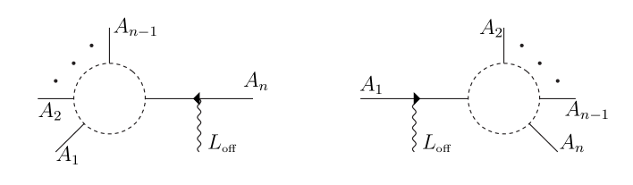
Figure 6: The remaining terms in the first case that does not cancel in the manner of Figure 4. The loop is ghost loop and has two directions.

Case 2. We need to consider the hollow triangle terms from $k_{\mbox{\tiny off}}\cdot V_{\mbox{\tiny off}}$ remaining from the above case, and we divide them into two sub cases:

Sub Case 1. When $V_{\mbox{\tiny off}}$ is not on the loop, these terms vanish due to Ward identity for less point amplitudes in the induction assumption, similar to the tree level counterpart Figure 3.

Sub Case 2. The remaining sub case is that $V_{\mbox{\tiny off}}$ is on the gauge field loop. We analyze one of the hollow triangle terms in Figure 7. The Figure has considered all the possible cases with the first right side vertex to be three or four point, and different types of second vertex relevant. When the first right side vertex is a three point vertex, acting on it with one of the factor in the hollow triangle term, we can again decompose it as in Figure 2 into solid and hollow triangle terms. (a) and (b) in Figure 7 are in fact the same diagrams as in Figure 4. (c) vanishes due to tree level Ward identity, and (d) is due to on shell condition for external legs besides $L_{\mbox{\tiny off}}$. Then the type of term in (e) of Figure 7 remains, which is a hollow triangle term staying on the loop, and it will act on the next vertex on the loop, repeating the same processes as in (a)-(d) of Figure 7, until it meets the final vertex on the loop. For this sub case, the remaining diagrams are in Figure 8.

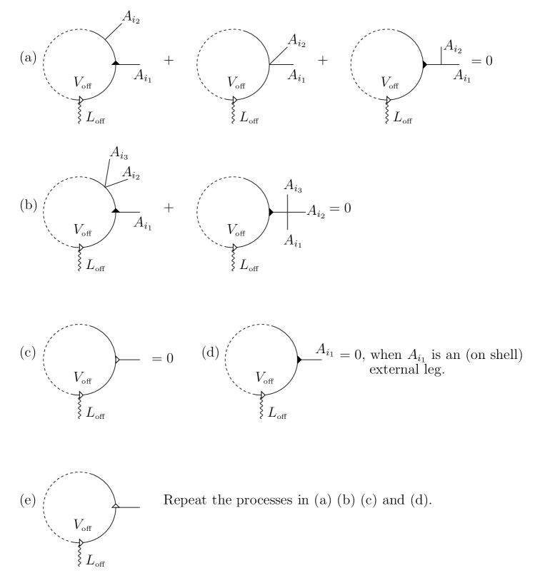
Figure 7: Analysis of the action of the hollow triangle terms in Sub Case 2. The dashed line is not ghost field, but just part of the loop diagram not relevant.

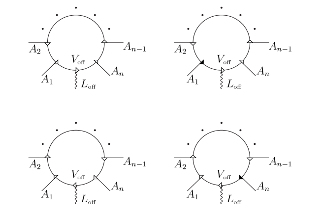
Figure 8: The terms from Sub Case 2. Except the hollow triangle terms at $V_{\mbox{\tiny off}}$, other hollow and solid triangle terms on the loop are induced from the hollow triangle term of the previous loop vertex, as described in the text of Sub Case 2. and Figure 7.

Case 3. The remaining case: $k_{\mbox{\tiny off}}$ is linked to a ghost propagator of the N point diagram, as in Figure 9.

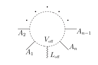
Figure 9: Diagram for Case 3. The ghost loop can be in two directions.

By direct and simple calculations, the terms from Figure 6, Figure 8 and Figure 9, with same set of sub amplitudes $A_{i}$, add up to be 0. Combine Case 1, 2, 3, we have proven that Ward identity holds at $N+1$ point one loop level. Thus by induction we have proven Ward identity holds at one loop level using Feynman rules in a direct way.

III.2 Recursion Relation for Loop Level Off Shell Amplitudes

Similar to the tree level off shell amplitudes calculation, we can use $\hat{A}_{\mu}\eta^{\mu}|_{z\rightarrow 0}=-{d\hat{A}_{\mu}\over dz}{\hat{k}}_{\mbox{\tiny off}}^{\mu}|_{z\rightarrow 0}$ to calculate one loop level off shell amplitudes. The experience at tree level, and the details of how Ward identity holds at one loop level discussed in the last subsection, help us to simplify our discussion and calculation of one loop level off shell amplitudes.

When the derivative acts on a gauge field propagator or a vertex which is not on the loop, we can use the expressions derived in section II.2 directly, ie. 9 and 10, for the contribution to $-{d\hat{A}_{\mu}\over dz}{\hat{k}}_{\mbox{\tiny off}}^{\mu}|_{z\rightarrow 0}$:

$$\frac{1}{2k_{A_{1}}^{2}k_{A_{2}}^{2}k_{A_{3}}^{2}}(A^{l/t}_{3}\cdot\eta\ A^{l/t}_{1}\cdot A^{l/t}_{2}+A^{l/t}_{1}\cdot\eta\ A^{l/t}_{2}\cdot A^{l/t}_{3}-2A^{l/t}_{2}\cdot\eta\ A^{l/t}_{1}\cdot A^{l/t}_{3}),$$ (13)

$$\frac{-i}{\sqrt{2}k_{A_{1}}^{2}k_{A_{2}}^{2}}\left(\ (k_{A_{1}}-k_{A_{2}})\cdot\eta\ A^{l/t}_{1}\cdot A^{l/t}_{2}+2A^{l/t}_{1}\cdot\eta\ k_{\mbox{\tiny off}}\cdot A^{l/t}_{2}-2A^{l/t}_{2}\cdot\eta\ k_{\mbox{\tiny off}}\cdot A^{l/t}_{1}\right).$$

In 13, we allocate the on shell external legs into $\{A^{l/t}_{i}\}$ in color ordering, with one and only one $A_{i}^{l/t}$ being one loop level. As in tree level, in each expression we should sum over all allowed allocations of the on shell external legs into $\{A^{l/t}_{i}\}$.

When the derivative acts on a gauge field loop propagator or a loop vertex, these are shown in Figure 10. For the same reasons as discussed in tree level recursion calculation, in (a) to (f), we only need to consider $L_{\mbox{\tiny off}}$ next to the propagator or vertex differentiated and only need the solid triangle term. In (g), we only differentiate the S and R terms of the vertex. The M part of the vertex in (g) will be dealt with in the following. In Figure 10, we encounter tree level two line off shell amplitudes $A^{t}_{\sigma\rho}$. This quantity can also be calculated recursively using our method, but in this paper we will not discuss it, and will use Feynman rules to calculate it in our example. Those $A^{t}$ without sub indices are tree level one line off shell amplitudes, which can apply our method in the previous section. (a) is 0 due to our convention for the loop momentum, described in the paragraph before section III.1.

Regardless of whether the other shifted line $L_{s}$ is among $\{L_{1},L_{2},\cdots,L_{j}\}$ or among $\{L_{j+1},\cdots,L_{N}\}$, the contributions to $-{d\hat{A}_{\mu}\over dz}{\hat{k}}_{\mbox{\tiny off}}^{\mu}|_{z\rightarrow 0}$ from Figure 10 are (we use $K_{m,n}$ to represent for $k_{m}+k_{m+1}+\cdots+k_{n}$):

$$(a)\ \ \ \ \ \ \ \,:0$$ (14)

$$(b)+(g):\frac{-i}{\sqrt{2}l^{2}(l+k_{\mbox{\tiny off}})^{2}}(\ (2l+k_{\mbox{\tiny off}})\cdot\eta\ A^{t}_{\sigma\rho}(1,2,\cdots,N)\ g^{\sigma\rho}$$

$$\ \ \ \ \ \ \ \ \ \ \ \ \ +2\eta^{\sigma}\ A^{t}_{\sigma\rho}(1,2,\cdots,N)\ k^{\rho}-2\eta^{\rho}\ A^{t}_{\sigma\rho}(1,2,\cdots,N)\ k^{\sigma})$$

$$(d)+(e):\frac{1}{2l^{2}(l-K_{1,j})^{2}K_{j+1,N}^{2}}(A^{t}(j+1,\cdots,N)\cdot\eta\ A^{t}_{\sigma\rho}(1,2,\cdots,j)\ g^{\sigma\rho}$$

$$\ \ \ \ \ \ \ \ \ \ \ \ \ -2A^{t\ \sigma}(j+1,\cdots,N)\ \eta^{\rho}\ A^{t}_{\sigma\rho}(1,2,\cdots,j)+A^{t\ \rho}(j+1,\cdots,N)\ \eta^{\sigma}\ A^{t}_{\sigma\rho}(1,2,\cdots,j)\ )$$

$$(c)+(f):\frac{1}{2(l+k_{\mbox{\tiny off}})^{2}(l-K_{1,j})^{2}K_{1,j}^{2}}(A^{t}(1,\cdots,j)\cdot\eta\ A^{t}_{\sigma\rho}(j+1,\cdots,N)\ g^{\sigma\rho}$$

$$\ \ \ \ \ \ \ \ \ \ \ \ \ -2A^{t\ \rho}(1,\cdots,j)\ \eta^{\sigma}\ A^{t}_{\sigma\rho}(j+1,\cdots,N)+A^{t\ \sigma}(1,\cdots,j)\ \eta^{\rho}\ A^{t}_{\sigma\rho}(j+1,\cdots,N)\ )$$

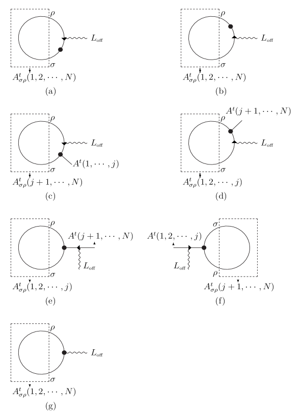
Figure 10: Diagrams with derivative acting on the propagator or vertex on the loop, which cannot directly apply the tree level results.

The final contributions to $-{d\hat{A}^{l}_{\mu}\over dz}{{\hat{k}}_{\mbox{\tiny off}}}^{\mu}|_{z\rightarrow 0}$ come from the derivatives in the diagrams of Figure 6, Figure 8 and Figure 9. Denoting the diagrams as $D_{i}$, since $\sum D_{i}\cdot k_{\mbox{\tiny off}}=0$ from the last subsection, we have $-\sum{d\hat{D}_{i\ \mu}\over dz}{\hat{k}}_{\mbox{\tiny off}}^{\mu}|_{z\rightarrow 0}=\sum D_{i\ \mu}\ \eta^{\mu}$. This is like an opposite operation compared to the method in the current paper to deal with the set of diagrams $D_{i}$, but it simplifies the local calculation, eg. the diagrams in Figure 6 turn out to be not contributing. We use $K_{A_{m,n}}$ to represent for $k_{A_{m}}+k_{A_{m+1}}+\cdots+k_{A_{n}}$, with $k_{A_{i}}$ the total momentum of the external legs contained in the sub amplitude $A_{i}$. The total momentum conservation is then $K_{A_{1,n}}+k_{\mbox{\tiny off}}=0$. The contributions to $-{d\hat{A}^{l}_{\mu}\over dz}{{\hat{k}}_{\mbox{\tiny off}}}^{\mu}|_{z\rightarrow 0}$ from derivatives in Figure 6, Figure 8 and Figure 9 are:

$$\frac{(-i)^{n}\ (l-K_{A_{1,1}})\cdot A_{2}\ (l-K_{A_{1,2}})\cdot A_{3}\ \cdots(l-K_{A_{1,n-2}})\cdot A_{n-1}}{(\sqrt{2})^{n+1}k_{A_{1}}^{2}\cdots k_{A_{n}}^{2}(l-K_{A_{1,1}})^{2}\cdots(l-K_{A_{1,n-1}})^{2}}$$

$$(-\frac{2l\cdot A_{1}\ (l-K_{A_{1,n-1}})\cdot A_{n}\ (2l+k_{\mbox{\tiny off}})\cdot\eta}{l^{2}(l+k_{\mbox{\tiny off}})^{2}}$$

$$+\frac{l\cdot A_{1}\ A_{n}\cdot\eta}{l^{2}}+\frac{(l-K_{A_{1,n-1}})\cdot A_{n}\ A_{1}\cdot\eta}{(l+k_{\mbox{\tiny off}})^{2}}).$$ (15)

This expression is well defined when $n\geq 2$. Especially when $n=2$, one should multiply the pre-factor with each term in the bracket to see that it is well defined. When $n=1$, the last two terms in the bracket vanish.

13, 14 and 15 constitute our expressions for recursively calculating one loop off shell amplitudes. In each expression, eg. in the above one 15, we should sum over all the allowed different allocations of the on shell external legs into $A_{1},\cdots,A_{n}$, with $n=1,2,\cdots,N$. This summation is not written explicitly in the expressions. Similar to our statement in the tree level counterpart, summing over 13, 14 and 15, we get a form $A^{l}_{\mu}\eta^{\mu}$, with the $A^{l}_{\mu}$ our wanted one loop off shell amplitude.

III.3 Examples of 1-loop Off Shell Amplitudes

As an application and verification of our method, we have computed three and four point one loop amplitudes with one off shell leg. ie. $A^{l}_{\mu}(k_{1},k_{2})$ and $A^{l}_{\mu}(k_{1},k_{2},k_{3})$, by summing up the contributions from 13, 14 and 15. We use the integral reduction method in Ellis to reduce the integrals to scalar integrals. We use the following notations for the scalar integrations:

$$B0[1,3]=\int\frac{d^{D}l}{(2\pi)^{D}}\frac{1}{l^{2}(l-k_{1}-k_{2})^{2}},\ \ B0[1,4]=\int\frac{d^{D}l}{(2\pi)^{D}}\frac{1}{l^{2}(l-k_{1}-k_{2}-k_{3})^{2}},$$

$$B0[2,4]=\int\frac{d^{D}l}{(2\pi)^{D}}\frac{1}{l^{2}(l-k_{2}-k_{3})^{2}},\ \ C0[1,2,3]=\int\frac{d^{D}l}{(2\pi)^{D}}\frac{1}{l^{2}(l-k_{1})^{2}(l-k_{1}-k_{2})^{2}},$$

$$C0[1,2,4]=\int\frac{d^{D}l}{(2\pi)^{D}}\frac{1}{l^{2}(l-k_{1})^{2}(l-k_{1}-k_{2}-k_{3})^{2}},$$

$$C0[1,3,4]=\int\frac{d^{D}l}{(2\pi)^{D}}\frac{1}{l^{2}(l-k_{1}-k_{2})^{2}(l-k_{1}-k_{2}-k_{3})^{2}},$$

$$C0[2,3,4]=\int\frac{d^{D}l}{(2\pi)^{D}}\frac{1}{l^{2}(l-k_{2})^{2}(l-k_{2}-k_{3})^{2}},$$

$$D0[1,2,3,4]=\int\frac{d^{D}l}{(2\pi)^{D}}\frac{1}{l^{2}(l-k_{1})^{2}(l-k_{1}-k_{2})^{2}(l-k_{1}-k_{2}-k_{3})^{2}}.$$

Other scalar integrations are not needed in this article. The evaluation of the scalar integrals see BernD2 .

We start from the two point function:

$$A^{l}_{\mu\nu}(k)=\frac{2-3D}{2(1-D)}(k^{2}g_{\mu\nu}-k_{\mu}k_{\nu})\int\frac{d^{D}l}{(2\pi)^{D}}\frac{1}{l^{2}(l-k)^{2}}.$$ (16)

Then we can calculate three point one loop off shell amplitude using our method:

$$A^{l}_{\mu}(k_{1},k_{2})=\frac{1}{2\sqrt{2}}\left[k_{1}\cdot\epsilon_{2}\ \epsilon_{1\ \mu}-k_{2}\cdot\epsilon_{1}\ \epsilon_{2\ \mu}-\frac{2D-5}{D-1}\epsilon_{1}\cdot\epsilon_{2}\ (k_{1}-k_{2})_{\mu}\right.$$

$$\ \ \ \ \ \ \ \ \ \ \ \ \ \ \ \ \ \ \ \ \ \ \ \ \ \left.+\frac{D-4}{D-1}\frac{k_{1}\cdot\epsilon_{2}\ k_{2}\cdot\epsilon_{1}}{k_{1}\cdot k_{2}}(k_{1}-k_{2})_{\mu}\right]B0[1,3]$$ (17)

$$\ \ \ \ \ \ \ \ \ \ \ \ \ \ \ +\frac{1}{2\sqrt{2}}k_{1}\cdot k_{2}[-3\epsilon_{1}\cdot\epsilon_{2}\ (k_{1}-k_{2})_{\mu}+4k_{1}\cdot\epsilon_{2}\ \epsilon_{1\ \mu}-4k_{2}\cdot\epsilon_{1}\ \epsilon_{2\ \mu}]C0[1,2,3].$$

At four point, the length of the expressions grow very quickly, and we will only give $A^{l}_{\mu}(1^{+},2^{+},3^{+})$. Instead of giving this expression directly, we will give $A^{l}_{\mu}(1^{+},2^{+},3^{+})\epsilon_{1}^{\mu}$, $A^{l}_{\mu}(1^{+},2^{+},3^{+})\epsilon_{3}^{\mu}$ and $A^{l}_{\mu}(1^{+},2^{+},3^{+})k_{1}^{\mu}$. Together with $A^{l}_{\mu}(1^{+},2^{+},3^{+})(k_{1}+k_{2}+k_{3})^{\mu}=0$, the expressions are enough to determine all the 4 components of $A^{l}_{\mu}(1^{+},2^{+},3^{+})$. We choose the spinor representations for $k_{1,2,3}$ and $\epsilon_{1,2,3}$ to be:

$$k_{1}=\lambda_{1}\tilde{\lambda}_{1},\ k_{2}=\lambda_{2}\tilde{\lambda}_{2},\ k_{3}=\lambda_{3}\tilde{\lambda}_{3},\ \epsilon_{1}=\frac{\lambda_{\nu}\tilde{\lambda}_{1}}{\langle\lambda_{\nu}\lambda_{1}\rangle},\ \epsilon_{2}=\frac{\lambda_{\nu}\tilde{\lambda}_{2}}{\langle\lambda_{\nu}\lambda_{2}\rangle},\ \epsilon_{3}=\frac{\lambda_{\nu}\tilde{\lambda}_{3}}{\langle\lambda_{\nu}\lambda_{3}\rangle},$$ (18)

with $\lambda_{\nu}$ an arbitrary reference spinor. We will use $\langle\nu 1\rangle$ to stand for $\langle\lambda_{\nu}\lambda_{1}\rangle$ and similarly others. We use $(A^{l}_{\mu}(1^{+},2^{+},3^{+})\epsilon_{1}^{\mu})_{D0[1,2,3,4]}$ to denote for the coefficient of $D0[1,2,3,4]$ in $A^{l}_{\mu}(1^{+},2^{+},3^{+})\epsilon_{1}^{\mu}$, and similarly for others. We give the coefficients at $D=4$. The off shell line makes the expressions much more complicated than that with all on shell lines. On one hand, when all lines are on shell, since the amplitudes are gauge invariant, we can choose some specific reference spinor, while in the off shell case we should keep the reference spinor $\lambda_{\nu}$ arbitrary. On the other hand, there are many terms in the expressions below which is 0 when all lines are on shell. For example, the first coefficient below would be 0 due to $(\langle 12\rangle[12]+\langle 13\rangle[13]+\langle 23\rangle[23])=0$ when all lines were on shell.

Then for $A^{l}_{\mu}(1^{+},2^{+},3^{+})\epsilon_{1}^{\mu}$:

$$(A^{l}_{\mu}(1^{+},2^{+},3^{+})\epsilon_{1}^{\mu})_{D0[1,2,3,4]}$$

$$=-\frac{(\langle 13\rangle\langle 2\nu\rangle-2\langle 12\rangle\langle 3\nu\rangle)[12](\langle 2\nu\rangle[12]+\langle 3\nu\rangle[13])[23](\langle 12\rangle[12]+\langle 13\rangle[13]+\langle 23\rangle[23])}{64\langle 13\rangle^{2}\langle 1\nu\rangle\langle 2\nu\rangle},$$

$$(A^{l}_{\mu}(1^{+},2^{+},3^{+})\epsilon_{1}^{\mu})_{C0[1,2,4]}$$

$$=-\frac{(\langle 2\nu\rangle[12]+\langle 3\nu\rangle[13])}{64\langle 12\rangle\langle 13\rangle^{2}\langle 1\nu\rangle^{2}\langle 23\rangle\langle 2\nu\rangle\langle 3\nu\rangle(\langle 12\rangle[12]+\langle 13\rangle[13])}(\langle 1\nu\rangle^{2}\langle 23\rangle^{2}(\langle 12\rangle\langle 13\rangle\langle 2\nu\rangle[12]^{2}+2\langle 12\rangle\langle 12\rangle\langle 3\nu\rangle[12]^{2}$$

$$+4\langle 12\rangle\langle 13\rangle\langle 3\nu\rangle[13][12]+\langle 13\rangle^{2}\langle 3\nu\rangle[13]^{2})[23]-\langle 1\nu\rangle(\langle 12\rangle[12]+\langle 13\rangle[13])(2\langle 3\nu\rangle^{2}[12]^{2}\langle 12\rangle^{3}+\langle 13\rangle\langle 3\nu\rangle[12](4\langle 3\nu\rangle[13]$$

$$-\langle 2\nu\rangle[12])\langle 12\rangle^{2}-2\langle 13\rangle^{2}\langle 2\nu\rangle[12](\langle 2\nu\rangle[12]+3\langle 3\nu\rangle[13])\langle 12\rangle-\langle 13\rangle^{3}\langle 2\nu\rangle\langle 3\nu\rangle[13]^{2})),$$

$$(A^{l}_{\mu}(1^{+},2^{+},3^{+})\epsilon_{1}^{\mu})_{C0[2,3,4]}$$

$$=-\frac{(\langle 2\nu\rangle[12]+\langle 3\nu\rangle[13])[23]}{64\langle 12\rangle\langle 13\rangle^{2}\langle 1\nu\rangle^{2}\langle 2\nu\rangle}(2\langle 3\nu\rangle(\langle 1\nu\rangle[12]-\langle 3\nu\rangle[23])\langle 12\rangle^{2}+\langle 13\rangle(-\langle 1\nu\rangle\langle 2\nu\rangle[12]+2\langle 1\nu\rangle\langle 3\nu\rangle[13]$$

$$+3\langle 2\nu\rangle\langle 3\nu\rangle[23])\langle 12\rangle+\langle 13\rangle^{2}\langle 2\nu\rangle(\langle 1\nu\rangle[13]+\langle 2\nu\rangle[23])),$$

$$(A^{l}_{\mu}(1^{+},2^{+},3^{+})\epsilon_{1}^{\mu})_{C0[1,3,4]}$$

$$=\frac{(\langle 2\nu\rangle[12]+\langle 3\nu\rangle[13])}{64\langle 12\rangle\langle 13\rangle^{2}\langle 1\nu\rangle^{2}\langle 23\rangle\langle 2\nu\rangle(\langle 13\rangle[13]+\langle 23\rangle[23])}(-2\langle 3\nu\rangle^{2}[12][23](2\langle 13\rangle[13]+\langle 23\rangle[23])\langle 12\rangle^{3}+\langle 3\nu\rangle(-2\langle 23\rangle^{2}\langle 3\nu\rangle[23]^{3}$$

$$+3\langle 13\rangle\langle 23\rangle(\langle 2\nu\rangle[12]-2\langle 3\nu\rangle[13])[23]^{2}+\langle 13\rangle^{2}[13](\langle 1\nu\rangle[12][13]-4\langle 3\nu\rangle[23][13]+4\langle 2\nu\rangle[12][23]))\langle 12\rangle^{2}+\langle 13\rangle\langle 2\nu\rangle\langle 3\nu\rangle[23](\langle 13\rangle^{2}[13]^{2}$$

$$+5\langle 13\rangle\langle 23\rangle[23][13]+3\langle 23\rangle^{2}[23]^{2})\langle 12\rangle+\langle 13\rangle^{2}\langle 2\nu\rangle(\langle 23\rangle^{2}\langle 2\nu\rangle[23]^{3}+3\langle 13\rangle\langle 23\rangle\langle 2\nu\rangle[13][23]^{2}+\langle 13\rangle^{2}[13]^{2}(\langle 1\nu\rangle[13]+3\langle 2\nu\rangle[23]))),$$

$$(A^{l}_{\mu}(1^{+},2^{+},3^{+})\epsilon_{1}^{\mu})_{C0[1,2,3]}$$

$$=\frac{[12](\langle 2\nu\rangle[12]+\langle 3\nu\rangle[13])}{64\langle 13\rangle^{2}\langle 1\nu\rangle^{2}\langle 23\rangle\langle 2\nu\rangle\langle 3\nu\rangle}(\langle 2\nu\rangle(2\langle 1\nu\rangle\langle 2\nu\rangle[12]+3\langle 1\nu\rangle\langle 3\nu\rangle[13]+\langle 2\nu\rangle\langle 3\nu\rangle[23])\langle 13\rangle^{2}$$

$$+\langle 12\rangle\langle 3\nu\rangle(\langle 1\nu\rangle\langle 2\nu\rangle[12]-2\langle 1\nu\rangle\langle 3\nu\rangle[13]-3\langle 2\nu\rangle\langle 3\nu\rangle[23])\langle 13\rangle+2\langle 12\rangle^{2}\langle 3\nu\rangle^{2}(\langle 3\nu\rangle[23]-\langle 1\nu\rangle[12])),$$

$$(A^{l}_{\mu}(1^{+},2^{+},3^{+})\epsilon_{1}^{\mu})_{B0[2,4]}$$

$$=-\frac{(\langle 2\nu\rangle[12]+\langle 3\nu\rangle[13])}{64\langle 12\rangle\langle 13\rangle\langle 1\nu\rangle^{2}\langle 23\rangle\langle 2\nu\rangle\langle 3\nu\rangle(\langle 12\rangle[12]+\langle 13\rangle[13])^{2}}(4\langle 3\nu\rangle^{2}[12][13](\langle 1\nu\rangle[12]-\langle 3\nu\rangle[23])\langle 12\rangle^{3}+\langle 13\rangle(\langle 1\nu\rangle[12](2\langle 2\nu\rangle^{2}[12]^{2}$$

$$-6\langle 2\nu\rangle\langle 3\nu\rangle[13][12]+5\langle 3\nu\rangle^{2}[13]^{2})+\langle 3\nu\rangle(-4\langle 2\nu\rangle^{2}[12]^{2}+7\langle 2\nu\rangle\langle 3\nu\rangle[13][12]-2\langle 3\nu\rangle^{2}[13]^{2})[23])\langle 12\rangle^{2}$$

$$+\langle 13\rangle^{2}(\langle 1\nu\rangle[13](7\langle 2\nu\rangle^{2}[12]^{2}-6\langle 2\nu\rangle\langle 3\nu\rangle[13][12]+\langle 3\nu\rangle^{2}[13]^{2})+\langle 2\nu\rangle(3\langle 2\nu\rangle^{2}[12]^{2}-10\langle 2\nu\rangle\langle 3\nu\rangle[13][12]$$

$$+\langle 3\nu\rangle^{2}[13]^{2})[23])\langle 12\rangle+5\langle 13\rangle^{3}\langle 2\nu\rangle^{2}[12][13](\langle 1\nu\rangle[13]+\langle 2\nu\rangle[23])),$$

$$(A^{l}_{\mu}(1^{+},2^{+},3^{+})\epsilon_{1}^{\mu})_{B0[1,4]}$$

$$=\frac{(\langle 2\nu\rangle[12]+\langle 3\nu\rangle[13])}{64\langle 12\rangle\langle 13\rangle\langle 1\nu\rangle^{2}\langle 23\rangle\langle 2\nu\rangle\langle 3\nu\rangle(\langle 12\rangle[12]+\langle 13\rangle[13])^{2}(\langle 13\rangle[13]+\langle 23\rangle[23])^{3}}(-2\langle 3\nu\rangle^{3}[12]^{3}[13][23](3\langle 13\rangle[13]+2\langle 23\rangle[23])\langle 12\rangle^{5}$$

$$+\langle 3\nu\rangle^{2}[12]^{2}[13](-8\langle 23\rangle^{2}\langle 3\nu\rangle[23]^{3}+\langle 13\rangle\langle 23\rangle(5\langle 2\nu\rangle[12]-28\langle 3\nu\rangle[13])[23]^{2}+2\langle 13\rangle^{2}[13](\langle 1\nu\rangle[12][13]-14\langle 3\nu\rangle[23][13]$$

$$+5\langle 2\nu\rangle[12][23]))\langle 12\rangle^{4}-\langle 3\nu\rangle[12](4\langle 23\rangle^{3}\langle 3\nu\rangle^{2}[13][23]^{4}+4\langle 13\rangle\langle 23\rangle^{2}(\langle 2\nu\rangle^{2}[12]^{2}-3\langle 2\nu\rangle\langle 3\nu\rangle[13][12]+6\langle 3\nu\rangle^{2}[13]^{2})[23]^{3}$$

$$+2\langle 13\rangle^{2}\langle 23\rangle[13](6\langle 2\nu\rangle[12]-11\langle 3\nu\rangle[13])(\langle 2\nu\rangle[12]-2\langle 3\nu\rangle[13])[23]^{2}+\langle 13\rangle^{3}[13]^{2}(\langle 1\nu\rangle[12][13](3\langle 2\nu\rangle[12]-8\langle 3\nu\rangle[13])$$

$$+2(6\langle 2\nu\rangle^{2}[12]^{2}-28\langle 2\nu\rangle\langle 3\nu\rangle[13][12]+15\langle 3\nu\rangle^{2}[13]^{2})[23]))\langle 12\rangle^{3}+\langle 13\rangle(\langle 23\rangle^{3}\langle 3\nu\rangle(-4\langle 2\nu\rangle^{2}[12]^{2}+7\langle 2\nu\rangle\langle 3\nu\rangle[13][12]$$

$$-2\langle 3\nu\rangle^{2}[13]^{2})[23]^{4}+\langle 13\rangle\langle 23\rangle^{2}(\langle 2\nu\rangle^{3}[12]^{3}-32\langle 2\nu\rangle^{2}\langle 3\nu\rangle[13][12]^{2}+33\langle 2\nu\rangle\langle 3\nu\rangle^{2}[13]^{2}[12]-10\langle 3\nu\rangle^{3}[13]^{3})[23]^{3}$$

$$+\langle 13\rangle^{2}\langle 23\rangle[13](3\langle 2\nu\rangle^{3}[12]^{3}-72\langle 2\nu\rangle^{2}\langle 3\nu\rangle[13][12]^{2}+62\langle 2\nu\rangle\langle 3\nu\rangle^{2}[13]^{2}[12]-14\langle 3\nu\rangle^{3}[13]^{3})[23]^{2}+\langle 13\rangle^{3}[13]^{2}(\langle 1\nu\rangle[12][13](\langle 2\nu\rangle^{2}[12]^{2}$$

$$-14\langle 2\nu\rangle\langle 3\nu\rangle[13][12]+6\langle 3\nu\rangle^{2}[13]^{2})+(3\langle 2\nu\rangle^{3}[12]^{3}-64\langle 2\nu\rangle^{2}\langle 3\nu\rangle[13][12]^{2}+53\langle 2\nu\rangle\langle 3\nu\rangle^{2}[13]^{2}[12]-6\langle 3\nu\rangle^{3}[13]^{3})[23]))\langle 12\rangle^{2}$$

$$+\langle 13\rangle^{2}\langle 2\nu\rangle(\langle 23\rangle^{3}(3\langle 2\nu\rangle^{2}[12]^{2}-10\langle 2\nu\rangle\langle 3\nu\rangle[13][12]+\langle 3\nu\rangle^{2}[13]^{2})[23]^{4}+\langle 13\rangle\langle 23\rangle^{2}[13](\langle 3\nu\rangle[13]-15\langle 2\nu\rangle[12])(3\langle 3\nu\rangle[13]$$

$$-\langle 2\nu\rangle[12])[23]^{3}+3\langle 13\rangle^{2}\langle 23\rangle[13]^{2}(9\langle 2\nu\rangle^{2}[12]^{2}-26\langle 2\nu\rangle\langle 3\nu\rangle[13][12]+\langle 3\nu\rangle^{2}[13]^{2})[23]^{2}+\langle 13\rangle^{3}[13]^{3}(\langle 1\nu\rangle[12][13](6\langle 2\nu\rangle[12]$$

$$-11\langle 3\nu\rangle[13])+(21\langle 2\nu\rangle^{2}[12]^{2}-58\langle 2\nu\rangle\langle 3\nu\rangle[13][12]+\langle 3\nu\rangle^{2}[13]^{2})[23]))\langle 12\rangle+5\langle 13\rangle^{3}\langle 2\nu\rangle^{2}[12][13](\langle 23\rangle^{3}\langle 2\nu\rangle[23]^{4}$$

$$+4\langle 13\rangle\langle 23\rangle^{2}\langle 2\nu\rangle[13][23]^{3}+6\langle 13\rangle^{2}\langle 23\rangle\langle 2\nu\rangle[13]^{2}[23]^{2}+\langle 13\rangle^{3}[13]^{3}(\langle 1\nu\rangle[13]+4\langle 2\nu\rangle[23]))),$$

$$(A^{l}_{\mu}(1^{+},2^{+},3^{+})\epsilon_{1}^{\mu})_{B0[1,3]}$$

$$=-\frac{(\langle 2\nu\rangle[12]+\langle 3\nu\rangle[13])}{64\langle 12\rangle\langle 13\rangle\langle 1\nu\rangle^{2}\langle 23\rangle\langle 2\nu\rangle\langle 3\nu\rangle(\langle 13\rangle[13]+\langle 23\rangle[23])^{3}}(\langle 2\nu\rangle[13]^{2}(\langle 1\nu\rangle[13](\langle 2\nu\rangle[12]-\langle 3\nu\rangle[13])+\langle 2\nu\rangle(3\langle 2\nu\rangle[12]$$

$$-5\langle 3\nu\rangle[13])[23])\langle 13\rangle^{4}+[13](3\langle 23\rangle\langle 2\nu\rangle^{2}(\langle 2\nu\rangle[12]-3\langle 3\nu\rangle[13])[23]^{2}+\langle 12\rangle\langle 3\nu\rangle[13](\langle 1\nu\rangle[13](\langle 3\nu\rangle[13]-3\langle 2\nu\rangle[12])$$

$$+6\langle 2\nu\rangle(\langle 3\nu\rangle[13]-2\langle 2\nu\rangle[12])[23]))\langle 13\rangle^{3}+(\langle 23\rangle^{2}\langle 2\nu\rangle^{2}(\langle 2\nu\rangle[12]-7\langle 3\nu\rangle[13])[23]^{3}+6\langle 12\rangle\langle 23\rangle\langle 2\nu\rangle\langle 3\nu\rangle[13](\langle 3\nu\rangle[13]$$

$$-2\langle 2\nu\rangle[12])[23]^{2}+2\langle 12\rangle^{2}\langle 3\nu\rangle^{2}[13]^{2}(\langle 1\nu\rangle[12][13]-3\langle 3\nu\rangle[23][13]+5\langle 2\nu\rangle[12][23]))\langle 13\rangle^{2}-\langle 3\nu\rangle[23](6\langle 3\nu\rangle^{2}[12][13]^{2}\langle 12\rangle^{3}$$

$$+\langle 23\rangle\langle 3\nu\rangle[13](9\langle 3\nu\rangle[13]-5\langle 2\nu\rangle[12])[23]\langle 12\rangle^{2}+2\langle 23\rangle^{2}\langle 2\nu\rangle(2\langle 2\nu\rangle[12]-\langle 3\nu\rangle[13])[23]^{2}\langle 12\rangle+2\langle 23\rangle^{3}\langle 2\nu\rangle^{2}[23]^{3})\langle 13\rangle$$

$$-4\langle 12\rangle^{2}\langle 23\rangle\langle 3\nu\rangle^{3}[13][23]^{2}(\langle 12\rangle[12]+\langle 23\rangle[23])).$$

For $A^{l}_{\mu}(1^{+},2^{+},3^{+})\epsilon_{3}^{\mu}$:

$$(A^{l}_{\mu}(1^{+},2^{+},3^{+})\epsilon_{3}^{\mu})_{D0[1,2,3,4]}$$

$$=\frac{(\langle 13\rangle\langle 2\nu\rangle-2\langle 12\rangle\langle 3\nu\rangle)[12][23](\langle 1\nu\rangle[13]+\langle 2\nu\rangle[23])(\langle 12\rangle[12]+\langle 13\rangle[13]+\langle 23\rangle[23])}{64\langle 13\rangle^{2}\langle 2\nu\rangle\langle 3\nu\rangle},$$

$$(A^{l}_{\mu}(1^{+},2^{+},3^{+})\epsilon_{3}^{\mu})_{C0[1,2,4]}$$

$$=\frac{(\langle 1\nu\rangle[13]+\langle 2\nu\rangle[23])}{64\langle 12\rangle\langle 13\rangle^{2}\langle 1\nu\rangle\langle 23\rangle\langle 2\nu\rangle\langle 3\nu\rangle^{2}(\langle 12\rangle[12]+\langle 13\rangle[13])}(\langle 1\nu\rangle^{2}\langle 23\rangle^{2}(\langle 12\rangle(\langle 13\rangle\langle 2\nu\rangle+2\langle 12\rangle\langle 3\nu\rangle)[12]^{2}+4\langle 12\rangle\langle 13\rangle\langle 3\nu\rangle[13][12]$$

$$+\langle 13\rangle^{2}\langle 3\nu\rangle[13]^{2})[23]-\langle 1\nu\rangle(\langle 12\rangle[12]+\langle 13\rangle[13])(2\langle 3\nu\rangle^{2}[12]^{2}\langle 12\rangle^{3}+\langle 13\rangle\langle 3\nu\rangle[12](4\langle 3\nu\rangle[13]-\langle 2\nu\rangle[12])\langle 12\rangle^{2}$$

$$-2\langle 13\rangle^{2}\langle 2\nu\rangle[12](\langle 2\nu\rangle[12]+3\langle 3\nu\rangle[13])\langle 12\rangle-\langle 13\rangle^{3}\langle 2\nu\rangle\langle 3\nu\rangle[13]^{2})),$$

$$(A^{l}_{\mu}(1^{+},2^{+},3^{+})\epsilon_{3}^{\mu})_{C0[2,3,4]}$$

$$=\frac{[23](\langle 1\nu\rangle[13]+\langle 2\nu\rangle[23])}{64\langle 12\rangle\langle 13\rangle^{2}\langle 1\nu\rangle\langle 2\nu\rangle\langle 3\nu\rangle}(2\langle 3\nu\rangle(\langle 1\nu\rangle[12]-\langle 3\nu\rangle[23])\langle 12\rangle^{2}+\langle 13\rangle(-\langle 1\nu\rangle\langle 2\nu\rangle[12]+2\langle 1\nu\rangle\langle 3\nu\rangle[13]+3\langle 2\nu\rangle\langle 3\nu\rangle[23])\langle 12\rangle$$

$$+\langle 13\rangle^{2}\langle 2\nu\rangle(\langle 1\nu\rangle[13]+\langle 2\nu\rangle[23])),$$

$$(A^{l}_{\mu}(1^{+},2^{+},3^{+})\epsilon_{3}^{\mu})_{C0[1,3,4]}$$

$$=-\frac{1}{64\langle 12\rangle\langle 13\rangle^{2}\langle 1\nu\rangle\langle 23\rangle\langle 2\nu\rangle\langle 3\nu\rangle(\langle 13\rangle[13]+\langle 23\rangle[23])}(2\langle 3\nu\rangle^{3}[12][13][23]^{2}\langle 12\rangle^{4}+\langle 3\nu\rangle^{2}[23](2\langle 23\rangle(\langle 3\nu\rangle[13]-\langle 2\nu\rangle[12])[23]^{2}$$

$$+\langle 13\rangle[13](-4\langle 1\nu\rangle[12][13]+6\langle 3\nu\rangle[23][13]-9\langle 2\nu\rangle[12][23]))\langle 12\rangle^{3}+\langle 3\nu\rangle(-2\langle 23\rangle^{2}\langle 2\nu\rangle\langle 3\nu\rangle[23]^{4}+\langle 13\rangle\langle 23\rangle\langle 2\nu\rangle(3\langle 2\nu\rangle[12]$$

$$-11\langle 3\nu\rangle[13])[23]^{3}+\langle 13\rangle^{2}[13](\langle 1\nu\rangle^{2}[12][13]^{2}+\langle 1\nu\rangle(5\langle 2\nu\rangle[12]-4\langle 3\nu\rangle[13])[23][13]+\langle 2\nu\rangle(7\langle 2\nu\rangle[12]-15\langle 3\nu\rangle[13])[23]^{2}))\langle 12\rangle^{2}$$

$$+\langle 13\rangle\langle 2\nu\rangle\langle 3\nu\rangle[23](3\langle 23\rangle^{2}\langle 2\nu\rangle[23]^{3}+7\langle 13\rangle\langle 23\rangle\langle 2\nu\rangle[13][23]^{2}+\langle 13\rangle^{2}[13]^{2}(\langle 1\nu\rangle[13]+3\langle 2\nu\rangle[23]))\langle 12\rangle$$

$$+\langle 13\rangle^{2}\langle 2\nu\rangle(\langle 23\rangle^{2}\langle 2\nu\rangle^{2}[23]^{4}+4\langle 13\rangle\langle 23\rangle\langle 2\nu\rangle^{2}[13][23]^{3}+\langle 13\rangle^{2}[13]^{2}(\langle 1\nu\rangle^{2}[13]^{2}+4\langle 1\nu\rangle\langle 2\nu\rangle[23][13]+6\langle 2\nu\rangle^{2}[23]^{2}))),$$

$$(A^{l}_{\mu}(1^{+},2^{+},3^{+})\epsilon_{3}^{\mu})_{C0[1,2,3]}$$

$$=-\frac{[12](\langle 1\nu\rangle[13]+\langle 2\nu\rangle[23])}{64\langle 13\rangle^{2}\langle 1\nu\rangle\langle 23\rangle\langle 2\nu\rangle\langle 3\nu\rangle^{2}}(\langle 2\nu\rangle(2\langle 1\nu\rangle\langle 2\nu\rangle[12]+3\langle 1\nu\rangle\langle 3\nu\rangle[13]+\langle 2\nu\rangle\langle 3\nu\rangle[23])\langle 13\rangle^{2}+\langle 12\rangle\langle 3\nu\rangle(\langle 1\nu\rangle\langle 2\nu\rangle[12]$$

$$-2\langle 1\nu\rangle\langle 3\nu\rangle[13]-3\langle 2\nu\rangle\langle 3\nu\rangle[23])\langle 13\rangle+2\langle 12\rangle^{2}\langle 3\nu\rangle^{2}(\langle 3\nu\rangle[23]-\langle 1\nu\rangle[12])),$$

$$(A^{l}_{\mu}(1^{+},2^{+},3^{+})\epsilon_{3}^{\mu})_{B0[2,4]}$$

$$=\frac{(\langle 1\nu\rangle[13]+\langle 2\nu\rangle[23])}{64\langle 12\rangle\langle 13\rangle\langle 1\nu\rangle\langle 23\rangle\langle 2\nu\rangle\langle 3\nu\rangle^{2}(\langle 12\rangle[12]+\langle 13\rangle[13])^{2}}(4\langle 3\nu\rangle^{2}[12][13](\langle 1\nu\rangle[12]-\langle 3\nu\rangle[23])\langle 12\rangle^{3}+\langle 13\rangle(\langle 1\nu\rangle[12](2\langle 2\nu\rangle^{2}[12]^{2}$$

$$-6\langle 2\nu\rangle\langle 3\nu\rangle[13][12]+5\langle 3\nu\rangle^{2}[13]^{2})+\langle 3\nu\rangle(-4\langle 2\nu\rangle^{2}[12]^{2}+7\langle 2\nu\rangle\langle 3\nu\rangle[13][12]-2\langle 3\nu\rangle^{2}[13]^{2})[23])\langle 12\rangle^{2}+\langle 13\rangle^{2}(\langle 1\nu\rangle[13](7\langle 2\nu\rangle^{2}[12]^{2}$$

$$-6\langle 2\nu\rangle\langle 3\nu\rangle[13][12]+\langle 3\nu\rangle^{2}[13]^{2})+\langle 2\nu\rangle(3\langle 2\nu\rangle^{2}[12]^{2}-10\langle 2\nu\rangle\langle 3\nu\rangle[13][12]+\langle 3\nu\rangle^{2}[13]^{2})[23])\langle 12\rangle$$

$$+5\langle 13\rangle^{3}\langle 2\nu\rangle^{2}[12][13](\langle 1\nu\rangle[13]+\langle 2\nu\rangle[23])),$$

$$(A^{l}_{\mu}(1^{+},2^{+},3^{+})\epsilon_{3}^{\mu})_{B0[1,4]}$$

$$=-\frac{1}{64\langle 12\rangle\langle 13\rangle\langle 1\nu\rangle\langle 23\rangle\langle 2\nu\rangle\langle 3\nu\rangle^{2}(\langle 12\rangle[12]+\langle 13\rangle[13])^{2}(\langle 13\rangle[13]+\langle 23\rangle[23])^{2}}(-4\langle 3\nu\rangle^{3}[12]^{2}[13][23](\langle 1\nu\rangle[12][13]-2\langle 3\nu\rangle[23][13]$$

$$+\langle 2\nu\rangle[12][23])\langle 12\rangle^{5}+\langle 3\nu\rangle^{2}[12][13](4\langle 23\rangle\langle 3\nu\rangle(\langle 3\nu\rangle[13]-2\langle 2\nu\rangle[12])[23]^{3}+\langle 13\rangle(2\langle 1\nu\rangle^{2}[12]^{2}[13]^{2}+\langle 1\nu\rangle[12](7\langle 2\nu\rangle[12]$$

$$-20\langle 3\nu\rangle[13])[23][13]+(9\langle 2\nu\rangle^{2}[12]^{2}-40\langle 2\nu\rangle\langle 3\nu\rangle[13][12]+20\langle 3\nu\rangle^{2}[13]^{2})[23]^{2}))\langle 12\rangle^{4}+\langle 3\nu\rangle(-4\langle 23\rangle^{2}\langle 2\nu\rangle\langle 3\nu\rangle^{2}[12][13][23]^{4}$$

$$+\langle 13\rangle\langle 23\rangle(-4\langle 2\nu\rangle^{3}[12]^{3}+16\langle 2\nu\rangle^{2}\langle 3\nu\rangle[13][12]^{2}-31\langle 2\nu\rangle\langle 3\nu\rangle^{2}[13]^{2}[12]+2\langle 3\nu\rangle^{3}[13]^{3})[23]^{3}+\langle 13\rangle^{2}[13](\langle 1\nu\rangle^{2}[12]^{2}(8\langle 3\nu\rangle[13]$$

$$-3\langle 2\nu\rangle[12])[13]^{2}+\langle 1\nu\rangle[12](-11\langle 2\nu\rangle^{2}[12]^{2}+42\langle 2\nu\rangle\langle 3\nu\rangle[13][12]-24\langle 3\nu\rangle^{2}[13]^{2})[23][13]+(-13\langle 2\nu\rangle^{3}[12]^{3}+74\langle 2\nu\rangle^{2}\langle 3\nu\rangle[13][12]^{2}$$

$$-70\langle 2\nu\rangle\langle 3\nu\rangle^{2}[13]^{2}[12]+8\langle 3\nu\rangle^{3}[13]^{3})[23]^{2}))\langle 12\rangle^{3}+\langle 13\rangle(\langle 23\rangle^{2}\langle 2\nu\rangle\langle 3\nu\rangle(-4\langle 2\nu\rangle^{2}[12]^{2}+7\langle 2\nu\rangle\langle 3\nu\rangle[13][12]-2\langle 3\nu\rangle^{2}[13]^{2})[23]^{4}$$

$$+\langle 13\rangle\langle 23\rangle\langle 2\nu\rangle(\langle 2\nu\rangle^{3}[12]^{3}-35\langle 2\nu\rangle^{2}\langle 3\nu\rangle[13][12]^{2}+43\langle 2\nu\rangle\langle 3\nu\rangle^{2}[13]^{2}[12]-11\langle 3\nu\rangle^{3}[13]^{3})[23]^{3}+\langle 13\rangle^{2}[13](\langle 1\nu\rangle^{2}[12](\langle 2\nu\rangle^{2}[12]^{2}$$

$$-14\langle 2\nu\rangle\langle 3\nu\rangle[13][12]+6\langle 3\nu\rangle^{2}[13]^{2})[13]^{2}+\langle 1\nu\rangle(3\langle 2\nu\rangle^{3}[12]^{3}-58\langle 2\nu\rangle^{2}\langle 3\nu\rangle[13][12]^{2}+42\langle 2\nu\rangle\langle 3\nu\rangle^{2}[13]^{2}[12]-6\langle 3\nu\rangle^{3}[13]^{3})[23][13]$$

$$+\langle 2\nu\rangle(3\langle 2\nu\rangle^{3}[12]^{3}-84\langle 2\nu\rangle^{2}\langle 3\nu\rangle[13][12]^{2}+98\langle 2\nu\rangle\langle 3\nu\rangle^{2}[13]^{2}[12]-16\langle 3\nu\rangle^{3}[13]^{3})[23]^{2}))\langle 12\rangle^{2}+\langle 13\rangle^{2}\langle 2\nu\rangle(\langle 23\rangle^{2}\langle 2\nu\rangle(3\langle 2\nu\rangle^{2}[12]^{2}$$

$$-10\langle 2\nu\rangle\langle 3\nu\rangle[13][12]+\langle 3\nu\rangle^{2}[13]^{2})[23]^{4}+3\langle 13\rangle\langle 23\rangle\langle 2\nu\rangle[13](5\langle 2\nu\rangle^{2}[12]^{2}-17\langle 2\nu\rangle\langle 3\nu\rangle[13][12]+\langle 3\nu\rangle^{2}[13]^{2})[23]^{3}$$

$$+\langle 13\rangle^{2}[13]^{2}(\langle 1\nu\rangle^{2}[12](6\langle 2\nu\rangle[12]-11\langle 3\nu\rangle[13])[13]^{2}+\langle 1\nu\rangle(21\langle 2\nu\rangle^{2}[12]^{2}-53\langle 2\nu\rangle\langle 3\nu\rangle[13][12]+\langle 3\nu\rangle^{2}[13]^{2})[23][13]$$

$$+3\langle 2\nu\rangle(9\langle 2\nu\rangle^{2}[12]^{2}-31\langle 2\nu\rangle\langle 3\nu\rangle[13][12]+\langle 3\nu\rangle^{2}[13]^{2})[23]^{2}))\langle 12\rangle+5\langle 13\rangle^{3}\langle 2\nu\rangle^{2}[12][13](\langle 23\rangle^{2}\langle 2\nu\rangle^{2}[23]^{4}$$

$$+4\langle 13\rangle\langle 23\rangle\langle 2\nu\rangle^{2}[13][23]^{3}+\langle 13\rangle^{2}[13]^{2}(\langle 1\nu\rangle^{2}[13]^{2}+4\langle 1\nu\rangle\langle 2\nu\rangle[23][13]+6\langle 2\nu\rangle^{2}[23]^{2}))),$$

$$(A^{l}_{\mu}(1^{+},2^{+},3^{+})\epsilon_{3}^{\mu})_{B0[1,3]}$$

$$=\frac{1}{64\langle 12\rangle\langle 13\rangle\langle 1\nu\rangle\langle 23\rangle\langle 2\nu\rangle\langle 3\nu\rangle^{2}(\langle 13\rangle[13]+\langle 23\rangle[23])^{2}}(\langle 2\nu\rangle[13](\langle 1\nu\rangle^{2}(\langle 2\nu\rangle[12]-\langle 3\nu\rangle[13])[13]^{2}+\langle 1\nu\rangle\langle 2\nu\rangle(3\langle 2\nu\rangle[12]$$

$$-5\langle 3\nu\rangle[13])[23][13]+3\langle 2\nu\rangle^{2}(\langle 2\nu\rangle[12]-3\langle 3\nu\rangle[13])[23]^{2})\langle 13\rangle^{3}+(\langle 23\rangle\langle 2\nu\rangle^{3}(\langle 2\nu\rangle[12]-7\langle 3\nu\rangle[13])[23]^{3}+\langle 12\rangle\langle 3\nu\rangle[13](\langle 1\nu\rangle^{2}(\langle 3\nu\rangle[13]$$

$$-3\langle 2\nu\rangle[12])[13]^{2}+\langle 1\nu\rangle\langle 2\nu\rangle(5\langle 3\nu\rangle[13]-11\langle 2\nu\rangle[12])[23][13]+\langle 2\nu\rangle^{2}(11\langle 3\nu\rangle[13]-13\langle 2\nu\rangle[12])[23]^{2}))\langle 13\rangle^{2}+\langle 3\nu\rangle(-2\langle 23\rangle^{2}\langle 2\nu\rangle^{3}[23]^{4}$$

$$+4\langle 12\rangle\langle 23\rangle\langle 2\nu\rangle^{2}(\langle 3\nu\rangle[13]-\langle 2\nu\rangle[12])[23]^{3}+\langle 12\rangle^{2}\langle 3\nu\rangle[13](2\langle 1\nu\rangle^{2}[12][13]^{2}+\langle 1\nu\rangle(7\langle 2\nu\rangle[12]-5\langle 3\nu\rangle[13])[23][13]$$

$$+\langle 2\nu\rangle(9\langle 2\nu\rangle[12]-11\langle 3\nu\rangle[13])[23]^{2}))\langle 13\rangle-4\langle 12\rangle^{2}\langle 3\nu\rangle^{3}[13][23](\langle 23\rangle\langle 2\nu\rangle[23]^{2}+\langle 12\rangle(\langle 1\nu\rangle[12][13]-\langle 3\nu\rangle[23][13]+\langle 2\nu\rangle[12][23]))).$$

For $A^{l}_{\mu}(1^{+},2^{+},3^{+})k_{1}^{\mu}$:

$$(A^{l}_{\mu}(1^{+},2^{+},3^{+})k_{1}^{\mu})_{D0[1,2,3,4]}$$

$$=\frac{[12]}{64\langle 13\rangle^{2}\langle 1\nu\rangle\langle 2\nu\rangle\langle 3\nu\rangle}(\langle 2\nu\rangle(4\langle 2\nu\rangle[12]+5\langle 3\nu\rangle[13])\langle 13\rangle^{2}+3\langle 12\rangle\langle 2\nu\rangle\langle 3\nu\rangle[12]\langle 13\rangle-2\langle 12\rangle^{2}\langle 3\nu\rangle^{2}[12])[23](\langle 12\rangle\langle 1\nu\rangle[12]$$

$$+\langle 13\rangle\langle 1\nu\rangle[13]+\langle 13\rangle\langle 2\nu\rangle[23]-\langle 12\rangle\langle 3\nu\rangle[23]),$$

$$(A^{l}_{\mu}(1^{+},2^{+},3^{+})k_{1}^{\mu})_{C0[1,3,4]}$$

$$=\frac{1}{64\langle 12\rangle\langle 13\rangle^{2}\langle 1\nu\rangle\langle 23\rangle\langle 2\nu\rangle\langle 3\nu\rangle}(2\langle 3\nu\rangle^{2}[12]^{2}(\langle 3\nu\rangle[23]-\langle 1\nu\rangle[12])\langle 12\rangle^{4}+\langle 13\rangle\langle 3\nu\rangle[12](\langle 1\nu\rangle[12](3\langle 2\nu\rangle[12]-4\langle 3\nu\rangle[13])$$

$$+\langle 3\nu\rangle(2\langle 3\nu\rangle[13]-5\langle 2\nu\rangle[12])[23])\langle 12\rangle^{3}+\langle 13\rangle^{2}([13](\langle 3\nu\rangle[13]-8\langle 2\nu\rangle[12])[23]\langle 3\nu\rangle^{2}+\langle 1\nu\rangle[12](2\langle 2\nu\rangle[12]-\langle 3\nu\rangle[13])(\langle 2\nu\rangle[12]$$

$$+4\langle 3\nu\rangle[13]))\langle 12\rangle^{2}+\langle 13\rangle^{3}(\langle 1\nu\rangle[13](6\langle 2\nu\rangle^{2}[12]^{2}+9\langle 2\nu\rangle\langle 3\nu\rangle[13][12]-2\langle 3\nu\rangle^{2}[13]^{2})+\langle 2\nu\rangle(3\langle 2\nu\rangle^{2}[12]^{2}+2\langle 2\nu\rangle\langle 3\nu\rangle[13][12]$$

$$-6\langle 3\nu\rangle^{2}[13]^{2})[23])\langle 12\rangle+\langle 13\rangle^{4}\langle 2\nu\rangle[13](4\langle 2\nu\rangle[12]+5\langle 3\nu\rangle[13])(\langle 1\nu\rangle[13]+\langle 2\nu\rangle[23])),$$

$$(A^{l}_{\mu}(1^{+},2^{+},3^{+})k_{1}^{\mu})_{C0[2,3,4]}$$

$$=\frac{[23]}{64\langle 12\rangle\langle 13\rangle^{2}\langle 1\nu\rangle\langle 2\nu\rangle\langle 3\nu\rangle}(2\langle 3\nu\rangle^{2}[12](\langle 1\nu\rangle[12]-\langle 3\nu\rangle[23])\langle 12\rangle^{3}+\langle 13\rangle\langle 3\nu\rangle[12](-3\langle 1\nu\rangle\langle 2\nu\rangle[12]+2\langle 1\nu\rangle\langle 3\nu\rangle[13]$$

$$+5\langle 2\nu\rangle\langle 3\nu\rangle[23])\langle 12\rangle^{2}+\langle 13\rangle^{2}\langle 2\nu\rangle(2\langle 1\nu\rangle[12](2\langle 2\nu\rangle[12]+\langle 3\nu\rangle[13])-\langle 3\nu\rangle(9\langle 2\nu\rangle[12]+7\langle 3\nu\rangle[13])[23])\langle 12\rangle$$

$$+\langle 13\rangle^{3}\langle 2\nu\rangle(4\langle 2\nu\rangle[12]+5\langle 3\nu\rangle[13])(\langle 1\nu\rangle[13]+\langle 2\nu\rangle[23])),$$

$$(A^{l}_{\mu}(1^{+},2^{+},3^{+})k_{1}^{\mu})_{C0[1,3,4]}$$

$$=\frac{1}{64\langle 12\rangle\langle 13\rangle^{2}\langle 1\nu\rangle\langle 23\rangle\langle 2\nu\rangle\langle 3\nu\rangle(\langle 13\rangle[13]+\langle 23\rangle[23])}(2\langle 3\nu\rangle^{3}[12]^{2}[23](2\langle 13\rangle[13]+\langle 23\rangle[23])\langle 12\rangle^{4}+\langle 3\nu\rangle^{2}[12](2\langle 23\rangle^{2}\langle 3\nu\rangle[23]^{3}$$

$$+\langle 13\rangle\langle 23\rangle(6\langle 3\nu\rangle[13]-5\langle 2\nu\rangle[12])[23]^{2}-\langle 13\rangle^{2}[13](\langle 1\nu\rangle[12][13]-2\langle 3\nu\rangle[23][13]+10\langle 2\nu\rangle[12][23]))\langle 12\rangle^{3}-\langle 13\rangle\langle 3\nu\rangle(5\langle 23\rangle^{2}\langle 2\nu\rangle\langle 3\nu\rangle[12][23]^{3}$$

$$+2\langle 13\rangle\langle 23\rangle\langle 3\nu\rangle[13](9\langle 2\nu\rangle[12]+2\langle 3\nu\rangle[13])[23]^{2}+\langle 13\rangle^{2}[13]((2\langle 2\nu\rangle^{2}[12]^{2}+17\langle 2\nu\rangle\langle 3\nu\rangle[13][12]+6\langle 3\nu\rangle^{2}[13]^{2})[23]-\langle 1\nu\rangle[12][13](2\langle 2\nu\rangle[12]$$

$$+\langle 3\nu\rangle[13])))\langle 12\rangle^{2}+\langle 13\rangle^{2}(\langle 23\rangle^{2}\langle 2\nu\rangle\langle 3\nu\rangle(\langle 2\nu\rangle[12]-\langle 3\nu\rangle[13])[23]^{3}+\langle 13\rangle\langle 23\rangle\langle 2\nu\rangle(4\langle 2\nu\rangle^{2}[12]^{2}+3\langle 2\nu\rangle\langle 3\nu\rangle[13][12]-3\langle 3\nu\rangle^{2}[13]^{2})[23]^{2}$$

$$+\langle 13\rangle^{2}[13](\langle 1\nu\rangle[13](4\langle 2\nu\rangle^{2}[12]^{2}+5\langle 2\nu\rangle\langle 3\nu\rangle[13][12]+2\langle 3\nu\rangle^{2}[13]^{2})+\langle 2\nu\rangle(8\langle 2\nu\rangle^{2}[12]^{2}+3\langle 2\nu\rangle\langle 3\nu\rangle[13][12]-3\langle 3\nu\rangle^{2}[13]^{2})[23]))\langle 12\rangle$$

$$+\langle 13\rangle^{3}\langle 2\nu\rangle(4\langle 2\nu\rangle[12]+3\langle 3\nu\rangle[13])(\langle 23\rangle^{2}\langle 2\nu\rangle[23]^{3}+3\langle 13\rangle\langle 23\rangle\langle 2\nu\rangle[13][23]^{2}+\langle 13\rangle^{2}[13]^{2}(\langle 1\nu\rangle[13]+3\langle 2\nu\rangle[23]))),$$

$$(A^{l}_{\mu}(1^{+},2^{+},3^{+})k_{1}^{\mu})_{C0[1,2,3]}$$

$$=\frac{[12]}{64\langle 13\rangle^{2}\langle 1\nu\rangle\langle 23\rangle\langle 2\nu\rangle\langle 3\nu\rangle}(\langle 1\nu\rangle(\langle 12\rangle[12]+\langle 13\rangle[13])(\langle 2\nu\rangle(6\langle 2\nu\rangle[12]+5\langle 3\nu\rangle[13])\langle 13\rangle^{2}-3\langle 12\rangle\langle 2\nu\rangle\langle 3\nu\rangle[12]\langle 13\rangle+2\langle 12\rangle^{2}\langle 3\nu\rangle^{2}[12])$$

$$+(\langle 13\rangle\langle 2\nu\rangle-\langle 12\rangle\langle 3\nu\rangle)(\langle 2\nu\rangle(4\langle 2\nu\rangle[12]+3\langle 3\nu\rangle[13])\langle 13\rangle^{2}-3\langle 12\rangle\langle 2\nu\rangle\langle 3\nu\rangle[12]\langle 13\rangle+2\langle 12\rangle^{2}\langle 3\nu\rangle^{2}[12])[23]),$$

$$(A^{l}_{\mu}(1^{+},2^{+},3^{+})k_{1}^{\mu})_{B0[2,4]}$$

$$=\frac{1}{64\langle 12\rangle\langle 13\rangle\langle 1\nu\rangle\langle 23\rangle\langle 2\nu\rangle\langle 3\nu\rangle(\langle 12\rangle[12]+\langle 13\rangle[13])}(\langle 1\nu\rangle(\langle 12\rangle[12]+\langle 13\rangle[13])(5\langle 13\rangle^{2}[12][13]\langle 2\nu\rangle^{2}+4\langle 12\rangle^{2}\langle 3\nu\rangle^{2}[12][13]$$

$$+\langle 12\rangle\langle 13\rangle(2\langle 2\nu\rangle^{2}[12]^{2}-6\langle 2\nu\rangle\langle 3\nu\rangle[13][12]+\langle 3\nu\rangle^{2}[13]^{2}))+(5\langle 13\rangle^{3}[12][13]\langle 2\nu\rangle^{3}+13\langle 12\rangle^{2}\langle 13\rangle\langle 3\nu\rangle^{2}[12][13]\langle 2\nu\rangle$$

$$+\langle 12\rangle\langle 13\rangle^{2}(\langle 2\nu\rangle^{2}[12]^{2}-12\langle 2\nu\rangle\langle 3\nu\rangle[13][12]+\langle 3\nu\rangle^{2}[13]^{2})\langle 2\nu\rangle-4\langle 12\rangle^{3}\langle 3\nu\rangle^{3}[12][13])[23]),$$

$$(A^{l}_{\mu}(1^{+},2^{+},3^{+})k_{1}^{\mu})_{B0[1,4]}$$

$$=\frac{1}{64\langle 12\rangle\langle 13\rangle\langle 1\nu\rangle\langle 23\rangle\langle 2\nu\rangle\langle 3\nu\rangle(\langle 12\rangle[12]+\langle 13\rangle[13])(\langle 13\rangle[13]+\langle 23\rangle[23])^{3}}(2\langle 3\nu\rangle^{3}[12]^{3}[13][23](3\langle 13\rangle[13]+2\langle 23\rangle[23])\langle 12\rangle^{5}$$

$$+\langle 3\nu\rangle^{2}[12]^{2}[13](8\langle 23\rangle^{2}\langle 3\nu\rangle[23]^{3}-11\langle 13\rangle\langle 23\rangle(\langle 2\nu\rangle[12]-2\langle 3\nu\rangle[13])[23]^{2}-2\langle 13\rangle^{2}[13](\langle 1\nu\rangle[12][13]-10\langle 3\nu\rangle[23][13]+9\langle 2\nu\rangle[12][23]))\langle 12\rangle^{4}$$

$$+\langle 3\nu\rangle[12](4\langle 23\rangle^{3}\langle 3\nu\rangle^{2}[13][23]^{4}-4\langle 13\rangle\langle 23\rangle^{2}(\langle 2\nu\rangle^{2}[12]^{2}+7\langle 2\nu\rangle\langle 3\nu\rangle[13][12]-4\langle 3\nu\rangle^{2}[13]^{2})[23]^{3}+2\langle 13\rangle^{2}\langle 23\rangle[13](-2\langle 2\nu\rangle^{2}[12]^{2}$$

$$-42\langle 2\nu\rangle\langle 3\nu\rangle[13][12]+11\langle 3\nu\rangle^{2}[13]^{2})[23]^{2}+\langle 13\rangle^{3}[13]^{2}(\langle 1\nu\rangle[12][13](5\langle 2\nu\rangle[12]-6\langle 3\nu\rangle[13])+2(2\langle 2\nu\rangle^{2}[12]^{2}-40\langle 2\nu\rangle\langle 3\nu\rangle[13][12]$$

$$+7\langle 3\nu\rangle^{2}[13]^{2})[23]))\langle 12\rangle^{3}+\langle 13\rangle(-\langle 23\rangle^{3}\langle 2\nu\rangle\langle 3\nu\rangle[12](4\langle 2\nu\rangle[12]+17\langle 3\nu\rangle[13])[23]^{4}+\langle 13\rangle\langle 23\rangle^{2}(\langle 2\nu\rangle^{3}[12]^{3}-2\langle 2\nu\rangle^{2}\langle 3\nu\rangle[13][12]^{2}$$

$$-83\langle 2\nu\rangle\langle 3\nu\rangle^{2}[13]^{2}[12]-4\langle 3\nu\rangle^{3}[13]^{3})[23]^{3}+\langle 13\rangle^{2}\langle 23\rangle[13](3\langle 2\nu\rangle^{3}[12]^{3}+26\langle 2\nu\rangle^{2}\langle 3\nu\rangle[13][12]^{2}-136\langle 2\nu\rangle\langle 3\nu\rangle^{2}[13]^{2}[12]$$

$$-8\langle 3\nu\rangle^{3}[13]^{3})[23]^{2}+\langle 13\rangle^{3}[13]^{2}(\langle 1\nu\rangle[12][13](\langle 2\nu\rangle^{2}[12]^{2}+18\langle 2\nu\rangle\langle 3\nu\rangle[13][12]-4\langle 3\nu\rangle^{2}[13]^{2})+(3\langle 2\nu\rangle^{3}[12]^{3}+42\langle 2\nu\rangle^{2}\langle 3\nu\rangle[13][12]^{2}$$

$$-91\langle 2\nu\rangle\langle 3\nu\rangle^{2}[13]^{2}[12]-4\langle 3\nu\rangle^{3}[13]^{3})[23]))\langle 12\rangle^{2}+\langle 13\rangle^{2}\langle 2\nu\rangle(\langle 23\rangle^{3}(3\langle 2\nu\rangle^{2}[12]^{2}+12\langle 2\nu\rangle\langle 3\nu\rangle[13][12]-5\langle 3\nu\rangle^{2}[13]^{2})[23]^{4}$$

$$+\langle 13\rangle\langle 23\rangle^{2}[13](3\langle 2\nu\rangle[12]-\langle 3\nu\rangle[13])(3\langle 2\nu\rangle[12]+19\langle 3\nu\rangle[13])[23]^{3}+9\langle 13\rangle^{2}\langle 23\rangle[13]^{2}(\langle 2\nu\rangle^{2}[12]^{2}+10\langle 2\nu\rangle\langle 3\nu\rangle[13][12]$$

$$-3\langle 3\nu\rangle^{2}[13]^{2})[23]^{2}+\langle 13\rangle^{3}[13]^{3}(17\langle 1\nu\rangle\langle 3\nu\rangle[12][13]^{2}+(3\langle 2\nu\rangle^{2}[12]^{2}+66\langle 2\nu\rangle\langle 3\nu\rangle[13][12]-17\langle 3\nu\rangle^{2}[13]^{2})[23]))\langle 12\rangle$$

$$-\langle 13\rangle^{3}\langle 2\nu\rangle[13](\langle 2\nu\rangle[12]-4\langle 3\nu\rangle[13])(\langle 23\rangle^{3}\langle 2\nu\rangle[23]^{4}+4\langle 13\rangle\langle 23\rangle^{2}\langle 2\nu\rangle[13][23]^{3}+6\langle 13\rangle^{2}\langle 23\rangle\langle 2\nu\rangle[13]^{2}[23]^{2}$$

$$+\langle 13\rangle^{3}[13]^{3}(\langle 1\nu\rangle[13]+4\langle 2\nu\rangle[23]))),$$

$$(A^{l}_{\mu}(1^{+},2^{+},3^{+})k_{1}^{\mu})_{B0[1,3]}$$

$$=-\frac{1}{64\langle 12\rangle\langle 13\rangle\langle 1\nu\rangle\langle 23\rangle\langle 2\nu\rangle\langle 3\nu\rangle(\langle 13\rangle[13]+\langle 23\rangle[23])^{3}}(2\langle 3\nu\rangle^{3}[12]^{2}[13][23](3\langle 13\rangle[13]+2\langle 23\rangle[23])\langle 12\rangle^{4}+\langle 3\nu\rangle^{2}[12][13](4\langle 23\rangle^{2}\langle 3\nu\rangle[23]^{3}$$

$$+\langle 13\rangle\langle 23\rangle(7\langle 3\nu\rangle[13]-11\langle 2\nu\rangle[12])[23]^{2}-2\langle 13\rangle^{2}[13](\langle 1\nu\rangle[12][13]-2\langle 3\nu\rangle[23][13]+9\langle 2\nu\rangle[12][23]))\langle 12\rangle^{3}$$

$$-\langle 13\rangle\langle 3\nu\rangle[13](2\langle 23\rangle^{2}\langle 3\nu\rangle(7\langle 2\nu\rangle[12]+2\langle 3\nu\rangle[13])[23]^{3}+\langle 13\rangle\langle 23\rangle(-8\langle 2\nu\rangle^{2}[12]^{2}+33\langle 2\nu\rangle\langle 3\nu\rangle[13][12]+9\langle 3\nu\rangle^{2}[13]^{2})[23]^{2}$$

$$+\langle 13\rangle^{2}[13](\langle 1\nu\rangle[12][13](\langle 3\nu\rangle[13]-5\langle 2\nu\rangle[12])+2(-8\langle 2\nu\rangle^{2}[12]^{2}+12\langle 2\nu\rangle\langle 3\nu\rangle[13][12]+3\langle 3\nu\rangle^{2}[13]^{2})[23]))\langle 12\rangle^{2}$$

$$+\langle 13\rangle(2\langle 23\rangle^{3}\langle 2\nu\rangle^{2}\langle 3\nu\rangle[12][23]^{4}+\langle 13\rangle\langle 23\rangle^{2}\langle 2\nu\rangle(-3\langle 2\nu\rangle^{2}[12]^{2}+13\langle 2\nu\rangle\langle 3\nu\rangle[13][12]+2\langle 3\nu\rangle^{2}[13]^{2})[23]^{3}$$

$$+3\langle 13\rangle^{2}\langle 23\rangle\langle 2\nu\rangle[13](-3\langle 2\nu\rangle^{2}[12]^{2}+9\langle 2\nu\rangle\langle 3\nu\rangle[13][12]+2\langle 3\nu\rangle^{2}[13]^{2})[23]^{2}+\langle 13\rangle^{3}[13]^{2}(\langle 1\nu\rangle[13](-3\langle 2\nu\rangle^{2}[12]^{2}+4\langle 2\nu\rangle\langle 3\nu\rangle[13][12]$$

$$+\langle 3\nu\rangle^{2}[13]^{2})+\langle 2\nu\rangle(-9\langle 2\nu\rangle^{2}[12]^{2}+23\langle 2\nu\rangle\langle 3\nu\rangle[13][12]+6\langle 3\nu\rangle^{2}[13]^{2})[23]))\langle 12\rangle-\langle 13\rangle^{2}\langle 2\nu\rangle(2\langle 23\rangle^{3}\langle 2\nu\rangle(2\langle 2\nu\rangle[12]$$

$$+\langle 3\nu\rangle[13])[23]^{4}+\langle 13\rangle\langle 23\rangle^{2}\langle 2\nu\rangle[13](15\langle 2\nu\rangle[12]+7\langle 3\nu\rangle[13])[23]^{3}+3\langle 13\rangle^{2}\langle 23\rangle\langle 2\nu\rangle[13]^{2}(7\langle 2\nu\rangle[12]+3\langle 3\nu\rangle[13])[23]^{2}$$

$$+\langle 13\rangle^{3}[13]^{3}(\langle 1\nu\rangle[13](3\langle 2\nu\rangle[12]+\langle 3\nu\rangle[13])+\langle 2\nu\rangle(13\langle 2\nu\rangle[12]+5\langle 3\nu\rangle[13])[23]))).$$

We checked our four point amplitudes using the known simple results of $A^{l}(1^{+},2^{+},3^{+},4^{+})$ and $A^{l}(1^{+},2^{+},3^{+},4^{-})$ in Bern:1991aq ; Bern2 ; Kharel ; Mahlon:1993si .

IV Conclusion

We have discussed the Ward identity in detail for off shell amplitudes in pure Yang-Mills theory. We explicitly prove that the Ward identity with two complexified external lines holds at tree and one loop level using Feynman rules. Then we use the Ward identity to deduce recursion relations for off shell amplitudes at tree and one loop level. In this technique, three steps are important to simplify the calculation. First, according to the complexfied Ward identity, we can convert the calculation of the amplitudes to the calculation of derivative of the amplitudes. Second, we decompose the three point vertex which contains the off shell line into three terms, which simplifies many steps in our calculation. Thirdly, according to the cancellation details in the proof of complexified Ward identity, we find most terms from different diagrams cancel with each other. The number of remaining effective terms or diagrams are reduced. It turns out that the recursion relation we derive at tree level is equivalent to Berends-Giele recursion relation Berends:1987me . However, our expressions at 1-loop level are new. And we present 1-loop off shell three and four point amplitudes as examples of applying our method at 1-loop level.

Comparing with our previous work Chen , we find the technique in this article is more universal. Here we can obtain a recursion relation for the total amplitudes instead of just the boundary terms of the amplitudes, and we do not need to use BCFW recursion relation. Furthermore, for this technique, we do not need to avoid the unphysical poles from the polarization vectors of the shifted on shell leg which can also depend on $z$. Hence this technique works well for the amplitudes with any helicity structure and the momenta shifts are more general than the ones in Chen . In addition, this technique can be used for calculating one loop off shell amplitudes with any helicity structure.

In principle, it is possible to generalize our method to higher loop levels and to other theories such as QCD. The only obstruct is to classify all the cancellation details for the Ward identity with complexfied external momenta. We leave this to future work. Another extension is to combine our technique with other methods, such as unitary cut, generalized unitary cut, BCFW, OPP OPP etc. to further simplify the calculation in pure Yang-Mills theory.

Acknowledgement We thank Edna Cheung, Jens Fjelstad, Konstantin G. Savvidy for helpful discussions. This work is funded by the Priority Academic Program Development of Jiangsu Higher Education Institutions (PAPD), NSFC grant No. 10775067, Research Links Programme of Swedish Research Council under contract No. 348-2008-6049, the Chinese Central Government’s 985 Project grants for Nanjing University, the China Science Postdoc grant no. 020400383. the postdoc grants of Nanjing University 0201003020

References

- (1) G. Chen, Phys. Rev. D 86, 027701 (2012) [arXiv:1203.6281 [hep-th]].
- (2) S. J. Parke and T. R. Taylor, An Amplitude for Gluon Scattering, Phys. Rev. Lett. 56, 2459 (1986).
- (3) Z. Xu, D. H. Zhang and L. Chang, Helicity Amplitudes for Multiple Bremsstrahlung in Massless Nonabelian Gauge Theories, Nucl. Phys. B 291, 392 (1987).
- (4) F. A. Berends and W. T. Giele, Recursive Calculations for Processes with n Gluons, Nucl. Phys. B 306, 759 (1988).
- (5) D. A. Kosower, Nucl. Phys. B 335, 23 (1990).
- (6) L. J. Dixon, In *Boulder 1995, QCD and beyond* 539-582 [hep-ph/9601359].
- (7) E. Witten, Commun. Math. Phys. 252, 189 (2004) [hep-th/0312171].
- (8) R. Britto, F. Cachazo and B. Feng, Computing one-loop amplitudes from the holomorphic anomaly of unitarity cuts, Phys. Rev. D 71, 025012 (2005) [arXiv:hep-th/0410179].
- (9) R. Britto, F. Cachazo and B. Feng, Generalized unitarity and one-loop amplitudes in N = 4 super-Yang-Mills, Nucl. Phys. B 725, 275-305 (2005), [arXiv:hep-th/0412103].
- (10) R. Britto, F. Cachazo and B. Feng, New recursion relations for tree amplitudes of gluons, Nucl. Phys. B 715, 499-522 (2005), [arXiv:hep-th/0412308].
- (11) R. Britto, F. Cachazo, B. Feng and E. Witten, Direct proof of tree-level recursion relation in Yang-Mills theory, Phys. Rev. Lett. 94, 181602 (2005), [arXiv:hep-th/0501052].
- (12) S. D. Badger, E. W. N. Glover, V. V. Khoze and P. Svrcek, JHEP 0507, 025 (2005) [hep-th/0504159].
- (13) K. J. Ozeren and W. J. Stirling, Eur. Phys. J. C 48, 159 (2006) [hep-ph/0603071].
- (14) C. Schwinn, Phys. Rev. D 78, 085030 (2008) [arXiv:0809.1442 [hep-ph]].
- (15) G. Chen and K. G. Savvidy, Eur. Phys. J. C 72, 1952 (2012) [arXiv:1105.3851 [hep-th]].
- (16) G. Chen, Phys. Rev. D 83, 125005 (2011) [arXiv:1103.2518 [hep-th]].
- (17) Z. Bern, L. J. Dixon, D. C. Dunbar and D. A. Kosower, Nucl. Phys. B 425, 217 (1994) [hep-ph/9403226].
- (18) Z. Bern, L. J. Dixon, D. C. Dunbar and D. A. Kosower, Nucl. Phys. B 435, 59 (1995) [hep-ph/9409265].
- (19) Z. Bern, V. Del Duca, L. J. Dixon and D. A. Kosower, Phys. Rev. D 71, 045006 (2005) [hep-th/0410224].
- (20) Z. Bern, N. E. J. Bjerrum-Bohr, D. C. Dunbar and H. Ita, JHEP 0511, 027 (2005) [hep-ph/0507019].
- (21) Z. Bern and D. A. Kosower, Nucl. Phys. B 379, 451 (1992).
- (22) C. F. Berger, Z. Bern, L. J. Dixon, D. Forde and D. A. Kosower, Phys. Rev. D 74, 036009 (2006) [hep-ph/0604195].
- (23) N. Arkani-Hamed, J. L. Bourjaily, F. Cachazo, S. Caron-Huot and J. Trnka, JHEP 1101, 041 (2011) [arXiv:1008.2958 [hep-th]].
- (24) B. Feng and Z. Zhang, JHEP 1112, 057 (2011) [arXiv:1109.1887 [hep-th]].
- (25) R. K. Ellis, Z. Kunszt, K. Melnikov and G. Zanderighi, Phys. Rept. 518, 141 (2012) [arXiv:1105.4319 [hep-ph]].
- (26) Z. Bern, In *Boulder 1992, Proceedings, Recent directions in particle theory* 471-535. and Calif. Univ. Los Angeles - UCLA-93-TEP-05 (93,rec.May) 66 p. C [hep-ph/9304249].
- (27) S. Kharel and G. Siopsis, Phys. Rev. D 86, 025004 (2012) [arXiv:1111.5278 [hep-th]].
- (28) G. Ossola, C. G. Papadopoulos and R. Pittau, Nucl. Phys. B 763, 147 (2007) [hep-ph/0609007].
- (29) G. Mahlon, Phys. Rev. D 49, 4438 (1994) [hep-ph/9312276].