On dependence consistency of $\operatorname{CoVaR}$ and some other systemic risk measures

Abstract

This paper is dedicated to the consistency of systemic risk measures with respect to stochastic dependence. It compares two alternative notions of Conditional Value-at-Risk ($\operatorname{CoVaR}$) available in the current literature. These notions are both based on the conditional distribution of a random variable $Y$ given a stress event for a random variable $X$, but they use different types of stress events. We derive representations of these alternative $\operatorname{CoVaR}$ notions in terms of copulas, study their general dependence consistency and compare their performance in several stochastic models. Our central finding is that conditioning on $X\geq\operatorname{VaR}_{\alpha}(X)$ gives a much better response to dependence between $X$ and $Y$ than conditioning on $X=\operatorname{VaR}_{\alpha}(X)$. We prove general results that relate the dependence consistency of $\operatorname{CoVaR}$ using conditioning on $X\geq\operatorname{VaR}_{\alpha}(X)$ to well established results on concordance ordering of multivariate distributions or their copulas. These results also apply to some other systemic risk measures, such as the Marginal Expected Shortfall ($\mathrm{MES}$) and the Systemic Impact Index ($\mathrm{SII}$). We provide counterexamples showing that $\operatorname{CoVaR}$ based on the stress event $X=\operatorname{VaR}_{\alpha}(X)$ is not dependence consistent. In particular, if $(X,Y)$ is bivariate normal, then $\operatorname{CoVaR}$ based on $X=\operatorname{VaR}_{\alpha}(X)$ is not an increasing function of the correlation parameter. Similar issues arise in the bivariate $t$ model and in the model with $t$ margins and a Gumbel copula. In all these cases, $\operatorname{CoVaR}$ based on $X\geq\operatorname{VaR}_{\alpha}(X)$ is an increasing function of the dependence parameter.

1 Introduction

The present paper studies the notion of Conditional Value-at-Risk ($\operatorname{CoVaR}$) introduced by Adrian and Brunnermeier [2] as a dependence adjusted version of Value-at-Risk ($\operatorname{VaR}$). The general idea behind $\operatorname{CoVaR}$ is to use the conditional distribution of a random variable $Y$ representing a particular financial institution (or the entire financial system) given that another institution, represented by a random variable $X$, is in stress. $\operatorname{CoVaR}$ represents one of the major threads in the current regulatory and scientific discussion of systemic risk, which significantly intensified after the recent financial crisis. The current discussion on systemic risk measurement is far from being concluded, and the competing methodologies are still under development. In addition to systemic risk measures [cf. 2, 4, 14, 15, 1, 29, 16], related topics include the structure of interbank networks, e.g., [8, 11], models explaining how systemic risk is created, e.g., [10, 17], and attribution of systemic risk charges within a financial system, as discussed in [26, 25].

Our contribution addresses the consistency of systemic risk measures with respect to the dependence in the underlying stochastic model. In the case of $\operatorname{CoVaR}$ we give a strong indication for the choice of the stress event for the conditioning random variable $X$. There are two alternative definitions of $\operatorname{CoVaR}$ in the current literature. The original definition in [2, 3, 4] is derived from the conditional distribution of $Y$ given that $X=\operatorname{VaR}_{\alpha}(X)$. The second one uses conditioning on $X\geq\operatorname{VaR}_{\alpha}(X)$. This modification was proposed by Girardi and Ergün [14] to improve the compatibility of $\operatorname{CoVaR}$ with non-parametric estimation methods. For similar reasons, such as continuity and better compatibility with discrete distributions, conditioning on $X\geq\operatorname{VaR}_{\alpha}(X)$ was also favoured by Klyman [20] for both $\operatorname{CoVaR}$ and Conditional Expected Shortfall ($\operatorname{CoES}$). Finally, it is remarkable that most competitors of $\operatorname{CoVaR}$ [cf. 15, 1, 29, 16] use conditioning on $X\geq\operatorname{VaR}_{\alpha}(X)$ as well. This approach goes in line with the general concept of stress scenarios discussed in [6].

Our results show that conditioning on $X\geq\operatorname{VaR}_{\alpha}(X)$ has great advantages for dependence modelling. We prove that this modification of $\operatorname{CoVaR}$ makes it response consistently to dependence parameters in many important stochastic models, whereas the original definition of $\operatorname{CoVaR}$ fails to do so. The counterexamples even include the bivariate Gaussian model, where the original $\operatorname{CoVaR}$ is decreasing with respect to the correlation $\rho:=\operatorname{corr}(X,Y)$ for $\rho>1/\sqrt{2}$. Thus, $\operatorname{CoVaR}$ based on $\{X=\operatorname{VaR}_{\alpha}(X)\}$ fails to detect systemic risk when it is most pronounced; and we also found this kind of inconsistency in other examples. On the other hand, our findings for the modified $\operatorname{CoVaR}$ relate its dependence consistency to concordance ordering of multivariate distributions or related copulas. This may explain the comparative results in [13], where $\operatorname{CoVaR^{=}}$ stood somewhat apart from its competitors. Moreover, it gives the the modified notion of $\operatorname{CoVaR}$ a solid mathematical basis.

Besides $\operatorname{CoVaR}$, we also discuss extensions to Conditional Expected Shortfall ($\operatorname{CoES}$). It turns out that the dependence inconsistency or dependence consistency of the alternative $\operatorname{CoVaR}$ notions is propagated to the corresponding definitions of $\operatorname{CoES}$. The dependence consistency results for $\operatorname{CoVaR}$ and $\operatorname{CoES}$ based on the stress scenario $X\geq\operatorname{VaR}_{\alpha}(X)$ also apply to the Marginal Expected Shortfall ($\mathrm{\operatorname{MES}}$) defined in [1] and to the Systemic Impact Index ($\mathrm{SII}$) introduced in [29].

The paper is organized as follows. Basic notation and alternative definitions of $\operatorname{CoVaR}$ and $\operatorname{CoES}$ are given in Section 2. In Section 3 we present the general mathematical results, including representations of $\operatorname{CoVaR}$ in terms of copulas and consistency of the modified $\operatorname{CoVaR}$ or $\operatorname{CoES}$ with respect to dependence characteristics. Section 4 contains a detailed comparison of the original and the modified $\operatorname{CoVaR}$ in three different models: the bivariate normal, the bivariate $t$ distribution, and a bivariate distribution with $t$ margins and a Gumbel copula. Conclusions are stated in Section 5.

2 Basic definitions and properties

Let $X$ and $Y$ be random variables representing the profits and losses of two financial institutions, such as banks. Focusing on risks, let $X$ and $Y$ be random loss variables, so that positive values of $X$ and $Y$ represent losses, whereas the gains are represented by negative values.

The issues of contagion and systemic stability raise questions for the joint probability distribution of $X$ and $Y$:

$$F_{X,Y}(x,y):=\mathrm{P}(X\leq x,Y\leq y).$$

The corresponding marginal distributions will be denoted by $F_{X}$ and $F_{Y}$. Provided a method to quantify the loss or gain of the entire financial system, $F_{X,Y}$ can also represent the joint loss distribution of a bank $X$ and the system $Y$.

In the current banking regulation framework (Basel II and the so-called Basel 2.5), the calculation of risk capital is based on measuring risk of each institution separately, with Value-at-Risk ($\operatorname{VaR}$) as a risk measure. The Value-at-Risk of a random loss $X$ at the confidence level $\alpha\in(0,1)$ is the $\alpha$-quantile of the loss distribution $F_{X}$ [cf. 21, Definition 2.10]. That is,

$$\operatorname{VaR}_{\alpha}(X)=F_{X}^{\leftarrow}(\alpha)$$

where $F_{X}^{\leftarrow}(y):=\inf\{x\in\mathbb{R}:F_{X}(x)\geq y\}$ is the generalized inverse of $F_{X}$. The most common values of $\alpha$ are $0.95$ and $0.99$.

For continuous and strictly increasing $F_{X}$ the generalized inverse $F_{X}^{\leftarrow}$ coincides with the inverse function $F_{X}^{-1}$ of $F_{X}$. In this case one has $\operatorname{VaR}_{\alpha}(X)=F_{X}^{-1}(\alpha)$ for $\alpha\in(0,1)$. For a thorough discussion of generalized inverse functions we refer to [12].

In the present paper we discuss two alternative approaches to adjust $\operatorname{VaR}$ to dependence between $X$ and $Y$. This is achieved by conditioning the distribution of $Y$ on a stress scenario for $X$. These two notions appear in the recent literature under the name Conditional Value-at-Risk ($\operatorname{CoVaR}$), but they use different kinds of stress scenarios. The original notion was introduced by Adrian and Brunnermeier [2, 3, 4] and will henceforth be denoted by $\operatorname{CoVaR^{=}}$. The alternative definition was proposed by Girardi and Ergün [14]. We denote it by $\operatorname{CoVaR}$.

Definition 2.1.

$$\operatorname{CoVaR_{\alpha,\beta}^{=}}(Y|X) :=\operatorname{VaR}_{\beta}(Y|X=\operatorname{VaR}_{\alpha}(X));$$

$$\operatorname{CoVaR_{\alpha,\beta}}(Y|X) :=\operatorname{VaR}_{\beta}(Y|X\geq\operatorname{VaR}_{\alpha}(X)).$$

The computation of $\operatorname{CoVaR^{=}}$ requires the knowledge of $F_{Y|X=\operatorname{VaR}_{\alpha}(X)}$. If $F_{X,Y}$ has a density $f_{X,Y}$, then $f_{X}(x)=\int_{-\infty}^{\infty}f_{X,Y}(x,y)dy$ is a density of $F_{X}$, and

$$F_{Y|X=\operatorname{VaR}_{\alpha}(X)}(y)=\frac{\int_{-\infty}^{y}f_{X,Y}(\operatorname{VaR}_{\alpha}(X),t)\,\text{d}t}{f_{X}(\operatorname{VaR}_{\alpha}(X))},$$

provided that $f_{X}(\operatorname{VaR}_{\alpha}(X))>0$. In some models, such as elliptical distributions, $F_{Y|X=\operatorname{VaR}_{\alpha}(X)}$ is known explicitly. In general, however, computation of $F_{Y|X=\operatorname{VaR}_{\alpha}(X)}$ requires numerical integration.

Conditioning on $X\geq\operatorname{VaR}_{\alpha}(X)$ is less technical. The definition of $\operatorname{VaR}_{\alpha}(X)$ implies that $\mathrm{P}(X\geq\operatorname{VaR}_{\alpha}(X))\geq 1-\alpha$, so that elementary conditional probabilities are well defined. In particular, if $F_{X}$ is continuous, then

$$F_{Y|X\geq\operatorname{VaR}_{\alpha}(X)}(y)=\frac{\mathrm{P}(Y\leq y,X\geq\operatorname{VaR}_{\alpha}(X))}{1-\alpha}.$$

Moreover, conditioning on events with positive probabilities is advantageous in statistical applications, including model fitting and backtesting. This is the major reason why the original notion of $\operatorname{CoVaR^{=}}$ was modified to $\operatorname{CoVaR}$ in [14].

A straightforward extension from $\operatorname{CoVaR}$ to Conditional Expected Shortfall ($\operatorname{CoES}$) is based on the representation $\operatorname{ES}_{\beta}(Y)=\frac{1}{1-\beta}\int_{\beta}^{1}\operatorname{VaR}_{t}(Y)dt$.

Definition 2.2.

$$\operatorname{CoES_{\alpha,\beta}}(Y|X) \colonequals\frac{1}{1-\beta}\int_{\beta}^{1}\operatorname{CoVaR}_{\alpha,t}(Y|X)\text{d}t,$$ (1)

$$\operatorname{CoES_{\alpha,\beta}^{=}}(Y|X) \colonequals\frac{1}{1-\beta}\int_{\beta}^{1}\operatorname{CoVaR^{=}}_{\alpha,t}(Y|X)\text{d}t.$$ (2)

Remark 2.3.

1. In precise mathematical terms, $\operatorname{CoVaR_{\alpha,\beta}^{=}}$ and $\operatorname{CoVaR_{\alpha,\beta}}$ are the $\beta$-quantiles of the conditional distributions $F_{Y|X=\operatorname{VaR}_{\alpha}(X)}$ and $F_{Y|X\geq\operatorname{VaR}_{\alpha}(X)}$:

   $$\operatorname{CoVaR_{\alpha,\beta}^{=}}(Y|X) =F_{Y|X=\operatorname{VaR}_{\alpha}(X)}^{\leftarrow}(\beta);$$

   $$\operatorname{CoVaR_{\alpha,\beta}}(Y|X) =F_{Y|X\geq\operatorname{VaR}_{\alpha}(X)}^{\leftarrow}(\beta).$$

2. In [2, 4, 18, 14], the authors work with a common confidence level for $X$ and $Y$, i.e., in the special case $\alpha=\beta$. Similarly to the notation used there, we will omit $\beta$ if $\beta=\alpha$ and write $\operatorname{CoVaR}_{\alpha}$ instead of $\operatorname{CoVaR}_{\alpha,\alpha}$ if it does not lead to confusion. However, the definition of $\operatorname{CoES}$ needs separate confidence levels for $X$ and $Y$ in the integrand $\operatorname{CoVaR}_{\alpha,t}(Y|X)$.

3. Since $\operatorname{CoES_{\alpha,\beta}}(Y|X)=\operatorname{ES}_{\beta}(Z)$ for a random variable $Z\sim F_{Y|X\geq\operatorname{VaR}_{\alpha}(X)}$, the coherence of $\operatorname{ES}$ in the sense of [5] is inherited by $\operatorname{CoES_{\alpha,\beta}}$ for all $\alpha,\beta\in(0,1)$. The central point here is subadditivity, which is understood as

   $$\operatorname{CoES_{\alpha,\beta}}(Y+Y^{\prime}|X)\leq\operatorname{CoES_{\alpha,\beta}}(Y|X)+\operatorname{CoES_{\alpha,\beta}}(Y^{\prime}|X)$$

   for any random variables $(Y,Y^{\prime},X)$ defined on the same probability space.

4. In [2, 4], $\operatorname{CoES}$ is defined as $\mathrm{E}[Y|Y\geq\operatorname{CoVaR_{\alpha,\alpha}^{=}}(Y|X)]$. Note that this definition replaces the stress scenario $\{X=\operatorname{VaR}_{\alpha}(X)\}$ by $\{Y\geq\operatorname{CoVaR_{\alpha,\alpha}^{=}}(Y|X)\}$, which is not related to $X$ directly. Compared to $\operatorname{CoES_{\alpha,\beta}^{=}}(Y|X)$, this definition is quite unnatural. Moreover, it does not guarantee coherence, which is the central property of Expected Shortfall.

5. The notion of Marginal Expected Shortfall ($\operatorname{MES}$) introduced in [1] is closely related to $\operatorname{CoVaR}$ and $\operatorname{CoES}$. It is defined as

   $$\operatorname{MES}_{\alpha}(Y|X):=\mathrm{E}[Y|X\geq\operatorname{VaR}_{\alpha}(X)]$$

   where $X:=\sum_{i=1}^{d}Y_{i}$ is the financial system and $Y:=Y_{i}$ for some $i$ is an institution. The idea behind $\operatorname{MES}$ is to quantify the insurance premia corresponding to bail-outs which become necessary when the entire financial system is close to a collapse. The major economic difference between $\operatorname{MES}$ and $\operatorname{CoVaR}$ is the role of $X$ and $Y$. With $\operatorname{MES}$, the conditioning random variable $X$ is the system, and the target random variable $Y$ is a part of the system. In the original work on $\operatorname{CoVaR}$, $Y$ is the system, and $X$ is a part of it.

   On the mathematical level, $\operatorname{MES}$ and $\operatorname{CoVaR}$ or $\operatorname{CoES}$ are quite close to each other. It is easy to see that

   $$\operatorname{MES}_{\alpha}(Y|X) =\int_{0}^{1}F_{Y|X\geq\operatorname{VaR}_{\alpha}(X)}^{\leftarrow}(t)dt=\int_{0}^{1}\operatorname{CoVaR}_{\alpha,t}(Y|X)dt.$$

   In view of (1), one could also write $\operatorname{MES}_{\alpha}(Y|X)=\operatorname{CoES}_{\alpha,0}(Y|X)$.

6. In [20], $\operatorname{CoVaR_{\alpha,\beta}}$ and $\operatorname{CoES_{\alpha,\beta}}$ in the sense of Definitions 2.1 and 2.2 are called $\mathrm{DistVaR}$ and $\mathrm{DistES}$. Besides the different naming, the definitions are essentially the same, and these notions are also compared to $\operatorname{CoVaR^{=}}$ and $\operatorname{CoES^{=}}$. However, the comparison in [20] is concentrated on general representations, compatibility with discrete, e.g., empirical, distributions, and the behaviour in the bivariate Black-Scholes model. As far as we are aware, a study of consistency with respect to dependence parameters has been missing so far.

The introduction of $\operatorname{CoVaR^{=}}$ in [2] aims not at $\operatorname{CoVaR^{=}}$ itself, but at the contribution of a particular financial institution to the systemic risk. In [2], $\operatorname{CoVaR^{=}}$ is used to construct a risk contribution measure that should quantify how a stress situation for an institution $X$ affects the system (or another institution) $Y$. In [2], the authors propose $\frac{\operatorname{CoVaR_{\alpha,\beta}^{=}}(Y|X)}{\operatorname{VaR}_{\beta}(Y)}-1$ as a systemic risk indicator. In [3], the systemic risk measure is modified to

$$\operatorname{\Delta CoVaR^{=}_{\alpha,\beta}}(Y|X):=\operatorname{CoVaR_{\alpha,\beta}^{=}}(Y)-\operatorname{VaR}_{\beta}(Y).$$ (3)

In [4], the centring term $\operatorname{VaR}_{\beta}(Y)$ representing the risk of $Y$ in an unstressed state is replaced by the conditional $\operatorname{VaR}$ of $Y$ given that $X$ is equal to its median:

$$\operatorname{\Delta^{\mathrm{med}}CoVaR^{=}_{\alpha,\beta}}(Y|X):=\operatorname{CoVaR_{\alpha,\beta}^{=}}(Y|X)-\operatorname{VaR}_{\beta}(Y|X=\operatorname{med}(X))$$ (4)

to remedy some inconsistencies observed in a comparison of $\operatorname{CoVaR^{=}}$ across different models.

Unfortunately, the centring in (3) is not the only reason why $\operatorname{\Delta CoVaR^{=}}$ can give a biased view of dependence between $X$ and $Y$. The results presented below demonstrate that there is a more fundamental issue that cannot be solved by modifying $\operatorname{\Delta CoVaR^{=}}$ to $\operatorname{\Delta^{\mathrm{med}}CoVaR^{=}}$ or taking any other centring term. The primary deficiency of $\operatorname{\Delta CoVaR^{=}}$ is that the underlying stress scenario $X=\operatorname{VaR}_{\alpha}(X)$ is too selective and over-optimistic. If, for instance, $F_{X}$ is continuous, then $\mathrm{P}(X=\operatorname{VaR}_{\alpha}(X))=0$, so that this particular event actually never occurs. Generally speaking, the ability of $\operatorname{CoVaR^{=}}$, $\operatorname{\Delta CoVaR^{=}}$, or $\operatorname{\Delta^{\mathrm{med}}CoVaR^{=}}$ to describe the influence of $X$ on $Y$ strongly depends on how well $F_{Y|X=\operatorname{VaR}_{\alpha}(X)}$ approximates $F_{Y|X=x}$ for $x\geq\operatorname{VaR}_{\alpha}(X)$. As shown in Section 4, this approximation fails even in very basic models, and it typically underestimates the contagion from $X$ to $Y$.

3 General results

We begin with representations of $\operatorname{CoVaR^{=}}$ and $\operatorname{CoVaR}$ in terms of copulas. It is well known that any bivariate distribution function $F_{X,Y}$ admits the decomposition

$$F_{X,Y}(x,y)=C(F_{X}(x),F_{Y}(y))$$ (5)

where $C$ is a probability distribution function on $(0,1)^{2}$ with uniform margins (cf. [24, 19]). That is, there exist random variables $U,V\sim\mathrm{unif}(0,1)$ such that $C(u,v)=\mathrm{P}(U\leq u,V\leq v)$. The function $C$ is called a copula of $F_{X,Y}$. If both $F_{X}$ and $F_{Y}$ are continuous, then $C$ is uniquely determined by $C(u,v)=F_{X,Y}(F_{X}^{\leftarrow}(u),F_{Y}^{\leftarrow}(v))$.

The decomposition (5) yields the following representation of $\operatorname{CoVaR^{=}}$ and $\operatorname{CoVaR}$.

Theorem 3.1.

Let $(U,V)\sim C$ where $C$ is a copula of $F_{X,Y}$. If $F_{X}$ is continuous, then

1. $\operatorname{CoVaR_{\alpha,\beta}^{=}}(Y|X)=F_{Y}^{\leftarrow}\left({F_{V|U=\alpha}^{\leftarrow}(\beta)}\right)$,

2. $\operatorname{CoVaR_{\alpha,\beta}}(Y|X)=F_{Y}^{\leftarrow}\left({F_{V|U\geq\alpha}^{\leftarrow}(\beta)}\right)$, and $F_{V|U\geq\alpha}(v)=\frac{v-C(\alpha,v)}{1-\alpha}$.

Proof.

Part (a). It is well known that $(F_{Y}^{\leftarrow}(U),F_{X}^{\leftarrow}(V))\sim F_{X,Y}$, and hence

$$F_{Y|X=\operatorname{VaR}_{\alpha}(X)}(y)=\mathrm{P}(F_{Y}^{\leftarrow}(V)\leq y|F_{X}^{\leftarrow}(U)=F_{X}^{\leftarrow}(\alpha)).$$

The functions $F_{Y}$ and $F_{Y}^{\leftarrow}$ are non-decreasing and satisfy $v\leq F_{Y}(F_{Y}^{\leftarrow}(v))$ and $F_{Y}^{\leftarrow}(F_{Y}(y))\leq y$ for all $v\in(0,1)$ and $y\in\mathbb{R}$. This implies that $F_{Y}^{\leftarrow}(V)\leq y$ is equivalent to $V\leq F_{Y}(y)$. Moreover, continuity of $F_{X}$ implies that $F_{X}^{\leftarrow}$ is strictly increasing, so that $F_{X}^{\leftarrow}(U)=F_{X}^{\leftarrow}(\alpha)$ is equivalent to $U=\alpha$. This yields

$$F_{Y|X=\operatorname{VaR}_{\alpha}(X)}(y)=\mathrm{P}(V\leq F_{Y}(y)|U=\alpha)=F_{V|U=\alpha}(F_{Y}(y)),$$

and the result follows from the chain rule for the generalized inverse.

Part(b). Analogously to Part (a), one obtains that

$$F_{Y|X\geq\operatorname{VaR}_{\alpha}(X)}(y)=\mathrm{P}(V\leq F_{Y}(y)|U\geq\alpha)=F_{V|U\geq\alpha}(F_{Y}(y)),$$

and hence $\operatorname{CoVaR_{\alpha,\beta}}(Y|X)=F_{Y}^{\leftarrow}(F_{V|U\geq\alpha}(\beta))$. Since $(U,V)\sim C$ and the margins of $C$ are uniform, we obtain that

$$F_{V|U\geq\alpha}(v) =\frac{P(V\leq v,U\geq\alpha)}{P(U\geq\alpha)}=\frac{v-C(\alpha,v)}{1-\alpha}.$$

∎

Theorem 3.1(a) provides a link between the ordering of $\operatorname{CoVaR}$ and the notion of concordance ordering.

Definition 3.2.

[cf. 22, Definition 3.8.1] Let $(X,Y)$ and $(X^{\prime},Y^{\prime})$ be bivariate random vectors with $F_{X}=F_{X^{\prime}}$ and $F_{Y}=F_{Y^{\prime}}$. Then $(X,Y)$ is smaller than $(X^{\prime},Y^{\prime})$ in concordance order ($(X,Y)\mathrel{\preceq}(X^{\prime},Y^{\prime})$ or, equivalently, $F_{X,Y}\mathrel{\preceq}F_{X^{\prime},Y^{\prime}}$) if

$$\forall x,y\in\mathbb{R}\quad\mathrm{P}(X\leq x,Y\leq y)\leq\mathrm{P}(X^{\prime}\leq x,Y^{\prime}\leq y).$$

Remark 3.3.

The following equivalent characterizations of $(X,Y)\mathrel{\preceq}(X^{\prime},Y^{\prime})$ will be used in in the sequel:

1. $P(X>x,Y>y)\leq P(X^{\prime}>x,Y^{\prime}>y)$ for all $x,y\in\mathbb{R}$;

2. $C\mathrel{\preceq}C^{\prime}$ for the copulas of $F_{X,Y}$ and $F_{X^{\prime},Y^{\prime}}$ if the margins are continuous;

3. $\mathrm{E}f(X,Y)\leq\mathrm{E}f(X^{\prime},Y^{\prime})$ for all supermodular functions $f:\mathbb{R}^{2}\to\mathbb{R}$, i.e., for all $f$ satisfying

   $$f(x+\varepsilon,y+\delta)+f(x,y)\geq f(x+\varepsilon,y)+f(x,y+\delta)$$

   for all $x,y\in\mathbb{R}$ and all $\varepsilon,\delta>0$. This order relation is called supermodular ordering ($\mathrel{\preceq}_{\mathrm{sm}}$).

For proofs and further alternative characterizations we refer to [22, Theorem 3.8.2].

The central theoretical result of the present paper is the following.

Theorem 3.4.

Let $(X,Y)$ and $(X^{\prime},Y^{\prime})$ be bivariate random vectors with copulas $C$ and $C^{\prime}$, respectively, and assume that $F_{Y}=F_{Y^{\prime}}$.

1. If $F_{X}$ and $F_{X^{\prime}}$ are continuous, then $C\mathrel{\preceq}C^{\prime}$ implies

   $$\forall\alpha,\beta\in(0,1)\quad\operatorname{CoVaR_{\alpha,\beta}}(Y|X)\leq\operatorname{CoVaR_{\alpha,\beta}}(Y^{\prime}|X^{\prime}).$$ (6)

2. If $F_{X}$, $F_{X^{\prime}}$, $F_{Y}$, and $F_{Y^{\prime}}$ are continuous, then (6) implies $C\mathrel{\preceq}C^{\prime}$.

Remark 3.5.

Note that Theorem 3.4 does not need $F_{X}=F_{X^{\prime}}$. The only assumption on the conditioning random variables $X$ and $X^{\prime}$ is that they are continuously distributed.

Proof.

Part (a). Let $(U,V)\sim C$ and $(U^{\prime},V^{\prime})\sim C^{\prime}$. As $F_{X}^{\leftarrow}$ and $F_{Y}^{\leftarrow}$ are non-decreasing, Theorem 3.1(b) reduces the problem to

$$\forall\alpha,\beta\in(0,1)\quad F_{V|U\geq\alpha}^{\leftarrow}(\beta)\leq F_{V^{\prime}|U^{\prime}\geq\alpha}^{\leftarrow}(\beta).$$ (7)

Moreover, it is well known that for any distribution functions $G$ and $H$ the ordering $G^{\leftarrow}(y)\leq H^{\leftarrow}(y)$ for all $y\in(0,1)$ is equivalent to $G(x)\geq H(x)$ for all $x\in\mathbb{R}$. Thus it suffices to show that

$$\forall\alpha,v\in(0,1)\quad F_{V|U\geq\alpha}(v)\geq F_{V^{\prime}|U^{\prime}\geq\alpha}(v).$$

The representation of $F_{V|U\alpha}(v)$ in Theorem 3.1(b) reduces this to $C(\alpha,v)\leq C^{\prime}(\alpha,v)$ for all $\alpha,v$, which is precisely $C\mathrel{\preceq}C^{\prime}$.

Part (b). Combining  (6) with Theorem 3.1, one obtains

$$\forall\alpha,\beta\quad F_{Y}^{\leftarrow}(F_{V|U\geq\alpha}^{\leftarrow}(\beta))\leq F_{Y}^{\leftarrow}(F_{V^{\prime}|U^{\prime}\geq\alpha}^{\leftarrow}(\beta)).$$ (8)

As $F_{Y}$ is continuous, $F_{Y}^{\leftarrow}$ is strictly increasing. Therefore (8) implies (7), which is equivalent to $C\mathrel{\preceq}C^{\prime}$. ∎

Theorem 3.4 can be applied to various stochastic models. We start with elliptical distributions. This model class includes such important examples as the multivariate Gaussian and the multivariate $t$ distributions. Since $\operatorname{CoVaR_{\alpha,\beta}}(X|Y)$ considers two random variables and multivariate ellipticity implies bivariate ellipticity for all bivariate sub-vectors, we restrict the consideration to the bivariate case.

A bivariate random vector $(X_{1},X_{2})$ is elliptically distributed if

$$(X,Y)^{\top}\stackrel{{\scriptstyle\mathrm{d}}}{{=}}\mu^{\top}+RAW^{\top}$$

where $\mu=(\mu_{X},\mu_{Y})\in\mathbb{R}^{2}$ and $A\in\mathbb{R}^{2\times 2}$ are constant, $W=(W_{1},W_{2})$ is uniformly distributed on the Euclidean unit sphere $\{x\in\mathbb{R}^{2}:\|x\|_{2}=1\}$, and $R$ is a non-negative random variable independent of $W$. If $\mathrm{E}R<\infty$, then $\mu_{X}=\mathrm{E}X$ and $\mu_{Y}=\mathrm{E}Y$. The ellipticity matrix $\Sigma:=A^{\top}A$ is unique except for a multiplicative factor. The covariance matrix of $(X,Y)$ is defined if and only if $\mathrm{E}R^{2}<\infty$, and this matrix is always equal to $c\Sigma$ for some constant $c>0$. Thus, rescaling $R$ and $A$, one can always achieve that

$$\Sigma=\left(\begin{array}[]{cc}\sigma_{X}^{2}&\sigma_{X}\sigma_{Y}\rho\\ \sigma_{X}\sigma_{Y}\rho&\sigma_{Y}^{2}\end{array}\right)$$ (9)

where, if defined, $\sigma_{X}=\operatorname{var}(X)$, $\sigma_{Y}=\operatorname{var}(Y)$, and $\rho=\operatorname{corr}(X,Y)$. In the following we will always assume this standardization of $\Sigma$ and denote the bivariate elliptical distribution with location parameter $\mu=(\mu_{X},\mu_{Y})$ and ellipticity matrix $\Sigma$ by $\mathcal{E}(\mu,\Sigma,R)$.

If $(X,Y)\sim\mathcal{E}(\mu,\Sigma,R)$ with continuous marginal distributions, then the copula $C$ of $(X,Y)$ is uniquely determined. Copulas of this type are called elliptical copulas. The invariance of copulas under increasing marginal transforms implies that $C$ depends only on the parameter $\rho$ of $\Sigma$ and on the distribution of $R$. Thus $\rho$ is the natural dependence parameter for a bivariate elliptical copula $C$, whereas the distribution of $R$ specifies the type of the copula, such as Gaussian or $t$. We will call elliptical copulas $C$ and $C^{\prime}$ of same type if the corresponding elliptical distributions have identical radial parts $R\stackrel{{\scriptstyle\mathrm{d}}}{{=}}R^{\prime}$.

The following theorem states monotonicity of $\operatorname{CoVaR}$ with respect to the dependence parameter $\rho$ if $(X,Y)$ is elliptically distributed or has an elliptical copula. In particular, it applies to bivariate Gaussian or bivariate $t$ distributions, and also to bivariate distributions with Gaussian or $t$ copulas.

Theorem 3.6.

1. Let $(X,Y)\sim\mathcal{E}(\mu,\Sigma,R)$ and $(X^{\prime},Y^{\prime})\sim\mathcal{E}(\mu^{\prime},\Sigma^{\prime},R)$ with continuous $F_{X}$ and $F_{X^{\prime}}$. If $\mu_{Y}\leq\mu_{Y^{\prime}}$ and $\sigma_{Y}=\sigma_{Y^{\prime}}$, then $\rho\leq\rho^{\prime}$ implies (6).

2. Let $(X,Y)\sim\mathcal{E}(\mu,\Sigma,R)$ and $(X^{\prime},Y^{\prime})\sim\mathcal{E}(\mu^{\prime},\Sigma^{\prime},R)$ with continuous $F_{X}$ and $F_{X^{\prime}}$. If $\mu_{Y}\leq\mu_{Y^{\prime}}$ and $\sigma_{Y}\leq\sigma_{Y^{\prime}}$, then $\rho\leq\rho^{\prime}$ implies

   $$\forall\alpha\in(0,1)\,\forall\beta\in[\beta_{0},1)\quad\operatorname{CoVaR_{\alpha,\beta}}(Y|X)\leq\operatorname{CoVaR_{\alpha,\beta}}(Y^{\prime}|X^{\prime})$$

   with $\beta_{0}:=\frac{1/2-C(\alpha,1/2)}{1-\alpha}$ where $C$ is the copula of $(X,Y)$.

3. Let $F_{X,Y}$ and $F_{X^{\prime},Y^{\prime}}$ have elliptical copulas of same type with dependence parameters $\rho$ and $\rho^{\prime}$, respectively. If $F_{X}$ and $F_{X^{\prime}}$ are continuous and $F_{Y}(y)\geq F_{Y^{\prime}}(y)$ for all $y\in\mathbb{R}$, then $\rho\leq\rho^{\prime}$ implies (6).

Remark 3.7.

1. The assumption $F_{Y}\geq F_{Y^{\prime}}$ obviously includes the case of identical margins $F_{Y}=F_{Y^{\prime}}$, which is the natural setting for studying the response of $\operatorname{CoVaR}$ to dependence parameters.

2. It is easy to see that the lower bound $\beta_{0}$ in Theorem 3.6(b) is decreasing in $\rho$. In particular, one has $\beta_{0}\leq 1/2$ for $\rho\geq 0$. This guarantees that $\operatorname{CoVaR_{\alpha,\beta}}(Y|X)\leq\operatorname{CoVaR_{\alpha,\beta}}(Y^{\prime}|X^{\prime})$ for $\alpha,\beta\in[1/2,1)$, which is fully sufficient for assessing dependence between rare events.

Proof of Theorem 3.6.

Part (a). It is obvious that $\operatorname{CoVaR_{\alpha,\beta}}(c+Y|X)=c+\operatorname{CoVaR_{\alpha,\beta}}(Y|X)$. Hence, as $\mu_{Y}\leq\mu_{Y^{\prime}}$, it suffices to consider $\mu_{Y}=\mu_{Y^{\prime}}$, so that we have $F_{Y}=F_{Y^{\prime}}$. Since the case $\sigma_{Y}=0$ is trivial, we only need to consider $\sigma_{Y}>0$.

The continuity of $F_{X}$ yields $\sigma_{X}>0$, and as $(X,Y)$ is elliptically distributed, we have $Y\stackrel{{\scriptstyle\mathrm{d}}}{{=}}\frac{\sigma_{Y}}{\sigma_{X}}X$. Hence $F_{Y}$ is continuous as well, and therefore the copulas $C$ and $C^{\prime}$ of $(X,Y)$ and $(X^{\prime},Y^{\prime})$ are uniquely defined.

According to Theorem 3.4(a), it suffices to show that $\rho<\rho^{\prime}$ implies $C\mathrel{\preceq}C^{\prime}$. This is equivalent to $\mathcal{E}(0,0,\Gamma(\rho),R)\mathrel{\preceq}\mathcal{E}(0,0,\Gamma(\rho^{\prime}),R)$ for $\rho\leq\rho^{\prime}$ and $\Gamma(\rho)=\left(\begin{array}[]{cc}1&\rho\\ \rho&1\end{array}\right)$. This ordering result is proven in [9]. In the bivariate Gaussian case it is also known as Slepian’s inequality [cf. 27, Theorem 5.1.7].

Part (b). Without loss of generality we can assume that $\mu_{Y}=\mu_{Y^{\prime}}$ and $\sigma_{Y}>0$. Part (a) gives us $C\mathrel{\preceq}C^{\prime}$ and hence (7). Moreover, $\sigma_{Y}\leq\sigma_{Y^{\prime}}$ implies that $F_{Y}^{\leftarrow}(t)\leq F_{Y^{\prime}}^{\leftarrow}(t)$ for $t\in[1/2,1)$. Hence, according to Theorem 3.1(b), it suffices to verify that $F_{V|U\geq\alpha}^{\leftarrow}(\beta)\geq 1/2$. This inequality is equivalent to $\beta\geq F_{V|U\geq\alpha}(1/2)=\beta_{0}$.

Part (c). According to Part (a), we have $C\mathrel{\preceq}C^{\prime}$ and hence (7). Since $F_{Y}(y)\geq F_{Y^{\prime}}(y)$ for all $y\in\mathbb{R}$ is equivalent to $F_{Y}(y)^{\leftarrow}(t)\leq F_{Y^{\prime}}^{\leftarrow}(t)$, Theorem 3.1(b) yields

$$\operatorname{CoVaR_{\alpha,\beta}}(Y|X)\leq F_{Y^{\prime}}^{\leftarrow}(F_{V|U\geq\alpha}^{\leftarrow}(\beta))\leq\operatorname{CoVaR_{\alpha,\beta}}(Y^{\prime}|X^{\prime}).$$

∎

A very popular copula model is the Gumbel copula. In the bivariate case it is defined as

$$C_{\theta}(u,v)=\exp\left({-\left({(-\log u)^{\theta}+(-\log v)^{\theta}}\right)^{1/\theta}}\right).$$ (10)

The dependence parameter $\theta$ assumes values in $[1,\infty]$, whereas $\theta=1$ and $\theta=\infty$ refer to $C_{1}(u,v):=uv$ (independence copula) and $C_{\infty}(u,v):=\min(u,v)$ (comonotonicity copula). As shown in [28], $\theta\leq\theta^{\prime}$ implies $C_{\theta}\mathrel{\preceq}_{\mathrm{sm}}C_{\theta^{\prime}}$ and hence $C_{\theta}\mathrel{\preceq}C_{\theta^{\prime}}$ (cf. Remark 3.3(c)). This immediately yields the following analogue of Theorem 3.6(c).

Corollary 3.8.

Let $(X,Y)$ and $(X^{\prime},Y^{\prime})$ have Gumbel copulas with dependence parameters $\theta$ and $\theta^{\prime}$, respectively. If $F_{X}$ and $F_{X^{\prime}}$ are continuous and $F_{Y}(y)\geq F_{Y^{\prime}}(y)$ for all $y\in\mathbb{R}$, then $\theta\leq\theta^{\prime}$ implies (6).

Remark 3.9.

Corollary 3.8 also holds for Galambos copulas with dependence parameters $\theta\leq\theta^{\prime}$; see [28] for $C_{\theta}\mathrel{\preceq}_{\mathrm{sm}}C_{\theta^{\prime}}$ in this case.

The monotonicity of $\operatorname{CoES_{\alpha,\beta}}(X,Y)$ with respect to dependence parameters follows from the integral representation (1).

Corollary 3.10.

Suppose that $\mathrm{E}|Y|$ and $\mathrm{E}|Y^{\prime}|$ are finite.

1. If $(X,Y)$ and $(X^{\prime},Y^{\prime})$ satisfy the assumptions of Theorem 3.6(a) or (c), or those of Corollary 3.8, then

   $$\forall\alpha,\beta\in(0,1)\quad\operatorname{CoES_{\alpha,\beta}}(Y|X)\leq\operatorname{CoES_{\alpha,\beta}}(Y^{\prime}|X^{\prime}).$$ (11)

2. If $(X,Y)$ and $(X^{\prime},Y^{\prime})$ satisfy the assumptions of Theorem 3.6(b), then

   $$\forall\alpha\in(0,1)\,\forall\beta\in[\beta_{0},1)\quad\operatorname{CoES_{\alpha,\beta}}(Y|X)\leq\operatorname{CoES_{\alpha,\beta}}(Y^{\prime}|X^{\prime}).$$

   with $\beta_{0}=\frac{1/2-C(\alpha,1/2)}{1-\alpha}$.

We conclude this section by relating the results obtained here to another systemic risk measure.

Remark 3.11.

1. Corollary 3.10(a) also applies to the Marginal Expected Shortfall from [1]. Setting $\beta=0$ in (11) and applying Remark 2.3(e), one obtains $\operatorname{MES}_{\alpha}(Y|X)\leq\operatorname{MES}_{\alpha}(Y^{\prime}|X^{\prime})$ for all $\alpha$.

2. In [29], the Systemic Impact Index ($\mathrm{SII}$) of an institution $Y_{i}$ is defined as

   $$\mathrm{SII}_{i}(\alpha) :=\mathrm{E}\left({\sum_{j=1}^{d}1\{Y_{j}\geq\operatorname{VaR}_{\alpha}(Y_{j})\}\bigg{|}Y_{i}\geq\operatorname{VaR}_{\alpha}(Y_{i})}\right)$$

   $$=1+\sum_{j\neq i}\mathrm{P}(Y_{j}\geq\operatorname{VaR}_{\alpha}(Y_{j})|Y_{i}\geq\operatorname{VaR}_{\alpha}(Y_{i})).$$

   It is easy to see that (6) is equivalent to

   $$\mathrm{P}(Y>\operatorname{VaR}_{\beta}(Y)|X>\operatorname{VaR}_{\beta}(X))\leq\mathrm{P}(Y^{\prime}>\operatorname{VaR}_{\beta}(Y^{\prime})|X^{\prime}>\operatorname{VaR}_{\beta}(X^{\prime}))$$

   for all $\alpha,\beta$. Thus, for $Y=Y_{j}$ and $X=Y_{i}$, the assumptions of Theorems 3.4(a) and 3.6 also imply dependence consistency of the single conditional default probabilities $\mathrm{P}(Y_{j}\geq\operatorname{VaR}_{\alpha}(Y_{j})|Y_{i}\geq\operatorname{VaR}_{\alpha}(Y_{i}))$.

4 Examples

In this section we compare $\operatorname{CoVaR}$ and $\operatorname{CoVaR^{=}}$ in three different models: the bivariate Gaussian, the bivariate $t$, and the bivariate distribution with a Gumbel copula and $t$ margins.

4.1 The bivariate Gaussian distribution

It is well known that the bivariate Gaussian distribution is elliptical. Hence Theorem 3.6(a) guarantees that $\operatorname{CoVaR}$ is an increasing function of the correlation parameter $\rho$. Moreover, $\operatorname{CoVaR^{=}}$ can be calculated explicitly in this case, so that it is particularly easy to compare $\operatorname{CoVaR}$ with $\operatorname{CoVaR^{=}}$.

Computation of $\operatorname{CoVaR^{=}}$

Let $(X,Y)\sim\mathcal{N}(\mu,\Sigma)$ with mean vector $\mu=(\mu_{X},\mu_{Y})$ and covariance matrix $\Sigma$ as in (9). As for all bivariate elliptical models, the dependence between $X$ and $Y$ is fully described by the correlation parameter $\rho$. An appealing property of the bivariate normal distribution is the interpretation as a linear model. Indeed, $(X,Y)\sim\mathcal{N}(\mu,\Sigma)$ is equivalent to

$$\frac{Y-\mu_{Y}}{\sigma_{Y}}=\rho\frac{X-\mu_{X}}{\sigma_{X}}+\sqrt{1-\rho^{2}}Z,$$ (12)

where $X\sim\mathcal{N}(\mu_{X},\sigma_{X}^{2})$ and $Z\sim\mathcal{N}(0,1)$, independent of $X$.

Due to $X\sim\mathcal{N}(\mu_{X},\sigma_{X}^{2})$ we have $\operatorname{VaR}_{\alpha}(X)=\mu_{X}+\sigma_{X}\Phi^{-1}(\alpha)$, where $\Phi$ is the distribution function of $\mathcal{N}(0,1)$. Substituting $X=\operatorname{VaR}_{\alpha}(X)$ in (12), one obtains

$$Y=\mu_{Y}+\sigma_{Y}\left({\rho\Phi^{-1}(\alpha)+\sqrt{1-\rho^{2}}Z}\right).$$

This shows that $\mathcal{L}(Y|X=\operatorname{VaR}_{\alpha}(X))=\mathcal{N}(\tilde{\mu},\tilde{\sigma}^{2})$ with $\tilde{\mu}=\mu_{Y}+\sigma_{Y}\rho\Phi^{-1}(\alpha)$ and $\tilde{\sigma}=\sigma_{Y}\sqrt{1-\rho^{2}}$. Hence we obtain that

$$\operatorname{CoVaR_{\alpha,\beta}^{=}}(Y|X) =\operatorname{VaR}_{\beta}(Y|X=\operatorname{VaR}_{\alpha}(X))=\tilde{\mu}+\tilde{\sigma}\Phi^{-1}(\beta)$$

$$=\mu_{Y}+\sigma_{Y}\left({\rho\Phi^{-1}(\alpha)+\Phi^{-1}(\beta)\sqrt{1-\rho^{2}}}\right).$$ (13)

Computation of $\operatorname{CoVaR}$

To compute $\operatorname{CoVaR}$, we use the copula representation from Theorem 3.1(b). From $Y\sim\mathcal{N}(\mu_{Y},\sigma^{2})$ one obtains that $F_{Y}^{-1}(v)=\mu_{Y}+\sigma_{Y}\Phi^{-1}(v)$ for $v\in(0,1)$. Moreover, the copula of $(X,Y)\sim\mathcal{N}(\mu,\Sigma)$ is the Gauss copula $C_{\rho}$ with dependence parameter $\rho$. For $\rho=0$ it is the independence copula, $C_{0}(u,v)=uv$, and for $\rho\neq 0$ it has the following representation:

$$C_{\rho}(u,v) =F_{X,Y}(F_{X}^{\leftarrow}(u),F_{Y}^{\leftarrow}(v))$$

$$=\int_{-\infty}^{\Phi^{-1}(v)}\int_{-\infty}^{\Phi^{-1}(u)}\frac{1}{2\pi\sqrt{1-\rho^{2}}}\exp\left({\frac{-(s_{1}^{2}-2\rho s_{1}s_{2}+s_{2}^{2})}{2(1-\rho^{2})}}\right)\text{d}s_{2}\text{d}s_{1}.$$ (14)

Applying Theorem 3.1(b), we obtain

$$\operatorname{CoVaR_{\alpha,\beta}}(Y)=\mu_{Y}+\sigma_{Y}\Phi^{-1}(F_{V|U\geq\alpha}^{-1}(\beta))$$

where $F_{V|U\geq\alpha}(v)=\frac{v-C_{\rho}(\alpha,v)}{1-\alpha}$. The values of $\operatorname{CoVaR}$ can be obtained by numerical integration of (14) and numerical inversion of the function $F_{V|U\geq\alpha}(v)$.

An alternative method to compute $\operatorname{CoVaR}$ is the numerical computation and inversion of the function

$$F_{Y|X\geq\operatorname{VaR}_{\alpha}(X)}(t)=\frac{1}{1-\alpha}\int_{-\infty}^{t}\int_{\operatorname{VaR}_{\alpha}(X)}^{\infty}f_{X,Y}(x,y)\,\text{d}x\,\text{d}y,$$ (15)

where $f_{X,Y}$ is the joint density of $X$ and $Y$. Depending on the application, each method has its advantages. Whilst (15) is more direct and hence faster for numerically tractable $f_{X,Y}$, the conditional copula values obtained in (14) can be re-used with other marginal distributions.

Monotonicity in $\rho$

As bivariate Gaussian distributions are elliptical, Theorem 3.6(a) guarantees that $\operatorname{CoVaR}$ is always increasing in $\rho$. However, this is not the case for $\operatorname{CoVaR^{=}}$. Partial differentiation of (13) in $\rho$ yields

$$\partial_{\rho}\operatorname{CoVaR_{\alpha,\beta}^{=}}(Y|X)=\sigma_{Y}\left({\Phi^{-1}(\alpha)-\frac{\rho\Phi^{-1}(\beta)}{\sqrt{1-\rho^{2}}}}\right),$$ (16)

which is positive if $\Phi^{-1}(\alpha)\sqrt{1-\rho^{2}}>\rho\Phi^{-1}(\beta)$ and negative if $\Phi^{-1}(\alpha)\sqrt{1-\rho^{2}}<\rho\Phi^{-1}(\beta)$. Besides the degenerate case $\alpha=\beta=1/2$ with constant $\operatorname{CoVaR_{\alpha,\beta}^{=}}$, there are 4 cases depending on the signs of $\Phi^{-1}(\alpha)$ and $\Phi^{-1}(\beta)$:

1. If $\alpha\geq 1/2$ and $\beta\geq 1/2$, then $\operatorname{CoVaR_{\alpha,\beta}^{=}}(Y|X)$ is increasing in $\rho$ for $\rho<\rho_{0}:=\frac{|\Phi^{-1}(\alpha)|}{\sqrt{(\Phi^{-1}(\alpha))^{2}+(\Phi^{-1}(\beta))^{2}}}$ and decreasing for $\rho>\rho_{0}$.

2. If $\alpha\geq 1/2$ and $\beta<1/2$, then $\operatorname{CoVaR_{\alpha,\beta}^{=}}(Y|X)$ is increasing in $\rho$ for $\rho>-\rho_{0}$ and decreasing for $\rho<-\rho_{0}$.

3. If $\alpha<1/2$ and $\beta\geq 1/2$, then $\operatorname{CoVaR_{\alpha,\beta}^{=}}(Y|X)$ is increasing in $\rho$ for $\rho<-\rho_{0}$ and decreasing for $\rho>-\rho_{0}$.

4. If $\alpha<1/2$ and $\beta<1/2$, then $\operatorname{CoVaR_{\alpha,\beta}^{=}}(Y|X)$ is increasing in $\rho$ for $\rho>\rho_{0}$ and decreasing for $\rho<\rho_{0}$.

Thus $\operatorname{CoVaR^{=}}$ is monotonic with respect to $\rho$ only in degenerate cases. In particular, in the most important case $\alpha,\beta\in(1/2,1)$, $\operatorname{CoVaR^{=}}$ is decreasing for $\rho>\rho_{0}$, which means that $\operatorname{CoVaR^{=}}$ fails to detect dependence where it is most pronounced. In the special case $\alpha=\beta$, the critical threshold $\rho_{0}$ is always equal to $1/\sqrt{2}$.

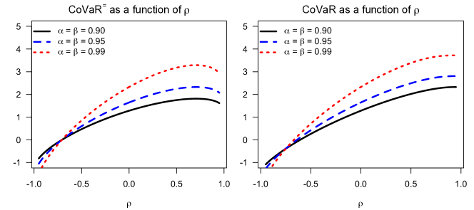
Figure 1: $\operatorname{CoVaR_{\alpha}^{=}}(Y|X)$ and $\operatorname{CoVaR_{\alpha}}(Y|X)$ (i.e., with $\beta=\alpha$) in the bivariate normal model as functions of $\rho$.

A graphic illustration to this fact is given in Figure 1, showing $\operatorname{CoVaR_{\alpha}^{=}}(Y|X)$ and $\operatorname{CoVaR_{\alpha}}(Y|X)$ for $\rho\geq 0.2$ and $\alpha=\beta$ assuming values $0.90,$ $0.95$, or $0.99$. The short writing $\operatorname{CoVaR_{\alpha}^{=}}$ refers to $\operatorname{CoVaR_{\alpha,\alpha}^{=}}$; analogously, $\operatorname{CoVaR_{\alpha}}$ denotes $\operatorname{CoVaR_{\alpha,\alpha}}$. This notation was used in the original definitions of $\operatorname{CoVaR^{=}}$ and $\operatorname{CoVaR}$, which were restricted to $\alpha=\beta$ (cf. Remark 2.3(b)). For the sake of simplicity we set $\mu_{Y}=0$ and $\sigma_{Y}=1$. These parameters have no influence on the decreasing or increasing behaviour of $\operatorname{CoVaR}$ or $\operatorname{CoVaR^{=}}$ as functions of $\rho$.

Normalized values of $\operatorname{CoVaR}$ and $\operatorname{CoVaR^{=}}$

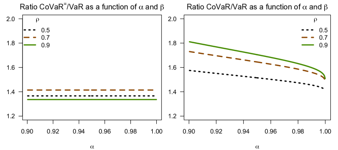
Figure 2: Bivariate normal model with $\mu_{Y}=0$: Ordering of the ratios $\operatorname{CoVaR_{\alpha}^{=}}(Y|X)/\operatorname{VaR}_{\alpha}(Y)$ and $\operatorname{CoVaR_{\alpha}}(Y|X)/\operatorname{VaR}_{\alpha}(Y)$ for different $\alpha$.

The relative impact of a stress event for $X$ on the institution $Y$ can be quantified by the ratio $\operatorname{CoVaR_{\alpha,\beta}^{=}}(Y|X)/\operatorname{VaR}_{\alpha}(Y)$ or by $\operatorname{CoVaR_{\alpha,\beta}}(Y|X)/\operatorname{VaR}_{\alpha}(Y)$. A similar of systemic risk indicator was proposed in [2]. Figure 2 shows these ratios for $\alpha=\beta$ and $\mu=0$ as functions of $\alpha$. The different line types in the plots correspond to $\rho=0.5$, $0.7$, and $0.92$. The ratios $\operatorname{CoVaR_{\alpha}^{=}}(Y|X)/\operatorname{VaR}_{\alpha}(Y)$ are constant, which is also easy to see from (13). The interesting part here is the ordering of the lines for different $\rho$. In case of $\operatorname{CoVaR^{=}}$, the line for $\rho=0.7$ is above the two others, illustrating that the inconsistency issue is common to all $\alpha\in(1/2,1)$. The plot of $\operatorname{CoVaR_{\alpha}}(Y|X)/\operatorname{VaR}_{\alpha}(Y)$ shows correct ordering for all $\alpha$, as guaranteed by Theorem 3.6(a). Another observation one can make here is that $\operatorname{CoVaR_{\alpha}}(Y|X)/\operatorname{VaR}_{\alpha}(Y)$ is decreasing in $\alpha$. This, however, is a model property that seems to be related to the light tail of the normal distribution. In heavy-tailed models considered in Sections 4.2 and 4.3 the ratio $\operatorname{CoVaR_{\alpha}}(Y|X)/\operatorname{VaR}_{\alpha}(Y)$ is increasing in $\alpha$.

Backtesting and violation rates

The results above show that $\operatorname{CoVaR}$ reflects the dependence between $X$ and $Y$ much more consistently than $\operatorname{CoVaR^{=}}$. An intuitive and very general explanation to this fact is that conditioning on $X\geq\operatorname{VaR}_{\alpha}(X)$ corresponds to a reasonable “what if” question, whereas conditioning on $X=\operatorname{VaR}_{\alpha}(X)$ does not. Indeed, the scenario $\{X\geq\operatorname{VaR}_{\alpha}(X)\}$ includes all possible outcomes for $X$ if $X$ is stressed, whereas the scenario $\{X=\operatorname{VaR}_{\alpha}(X)\}$ selects only the most benign of them.

In backtesting of $\operatorname{VaR}$ one expects that $X$ exceeds $\operatorname{VaR}_{\alpha}(X)$ with probability not larger than $1-\alpha$. Abbreviating “Conditional $\operatorname{VaR}$”, the term $\operatorname{CoVaR_{\alpha,\beta}^{=}}$ suggests that $Y$ exceeds $\operatorname{CoVaR_{\alpha,\beta}^{=}}(Y|X)$ with conditional probability $1-\beta$ or less, given that $X$ is stressed. The definition of $\operatorname{CoVaR}$ understands stress of $X$ as $\{X\geq\operatorname{VaR}_{\alpha}(X)\}$, so that the expected violation rate for $\operatorname{CoVaR_{\alpha,\beta}}$ under this stress scenario is equal to $1-\beta$. In contrast to that, $\operatorname{CoVaR^{=}}$ is designed to have the violation rate $1-\beta$ under the less natural and more optimistic scenario $\{X=\operatorname{VaR}_{\alpha}(X)\}$. As a consequence, the violation rates for $\operatorname{CoVaR_{\alpha,\beta}^{=}}$ backtesting experiments based on the natural stress scenario $\{X\geq\operatorname{VaR}_{\alpha}(X)\}$ are significantly higher than $1-\beta$.

This issue is illustrated in Table 1. The underlying Monte Carlo experiment generates an i.i.d. sample $(X_{i},Y_{i})\sim\mathcal{N}(0,\Sigma)$ for $i=1,\ldots,n$ and counts the joint exceedances $\{Y_{i}\geq\operatorname{CoVaR_{\alpha,\beta}^{=}}(Y|X),X_{i}\geq\operatorname{VaR}_{\alpha}(X)\}$. The $\operatorname{CoVaR^{=}}$ violation rate for the stress scenario $\{X\geq\operatorname{VaR}_{\alpha}(X)\}$ is the ratio of the joint excess count and the count of the excesses $\{X_{i}\geq\operatorname{VaR}_{\alpha}(X)\}$. The violation rate for $\operatorname{CoVaR}$ is obtained analogously from the number of joint exceedances $\{Y_{i}\geq\operatorname{CoVaR_{\alpha,\beta}}(Y|X),X_{i}\geq\operatorname{VaR}_{\alpha}(X)\}$. We chose $n=10^{7}$ and $\alpha,\beta$ being either $0.95$ or $0.99$.

It is remarkable that the violation rate for $\operatorname{CoVaR^{=}}$ increases with $\rho$. This demonstrates that the underestimation of risk by $\operatorname{CoVaR^{=}}$ is most pronounced in case of strong dependence and, hence, high systemic risk.

Bound	$\rho=0$	$\rho=0.2$	$\rho=0.5$	$\rho=0.7$	$\rho=0.9$
$\operatorname{CoVaR}_{0.95,0.95}^{=}(Y|X)$	0.0503	0.0601	0.0857	0.1229	0.2520
$\operatorname{CoVaR}_{0.99,0.99}^{=}(Y|X)$	0.0099	0.0124	0.0189	0.0292	0.0875
$\operatorname{CoVaR}_{0.95,0,99}^{=}(Y|X)$	0.0101	0.0130	0.0213	0.0375	0.1224
$\operatorname{CoVaR}_{0.99,0.95}^{=}(Y|X)$	0.0500	0.0588	0.0785	0.1045	0.2053
$\operatorname{CoVaR}_{0.95,0.95}(Y|X)$	0.0503	0.0500	0.0503	0.0495	0.0499
$\operatorname{CoVaR}_{0.99,0.99}(Y|X)$	0.0099	0.0101	0.0104	0.0099	0.0098
$\operatorname{CoVaR}_{0.95,0.99}(Y|X)$	0.0101	0.0102	0.0102	0.0099	0.0098
$\operatorname{CoVaR}_{0.99,0.95}(Y|X)$	0.0500	0.0507	0.0509	0.0501	0.0491

Table 1: Violation rates in the bivariate normal case. Monte Carlo backtesting with $n=10^{7}$ and $\alpha,\beta\in\{0.95,0.99\}$

A graphical illustration to this issue is given in Figure 3 by bivariate normal samples from the simulation study described above. The horizontal lines mark the levels of $\operatorname{CoVaR_{\alpha}^{=}}(Y|X)$ and $\operatorname{CoVaR_{\alpha}}(Y|X)$, and $\operatorname{VaR}_{\alpha}(Y)$. The vertical lines mark $\operatorname{VaR}_{\alpha}(X)$. The joint excess counts are the numbers of points above the corresponding horizontal line and on the right hand side from the vertical line marking $\operatorname{VaR}_{\alpha}(X)$. The sample size is $n=2000$, which suffices to demonstrate how correlation changes the shape of the sample cloud and thus increases the number of the joint excesses $\{Y_{i}\geq\operatorname{CoVaR_{\alpha}^{=}}(Y|X),X_{i}\geq\operatorname{VaR}_{\alpha}(X)\}$.

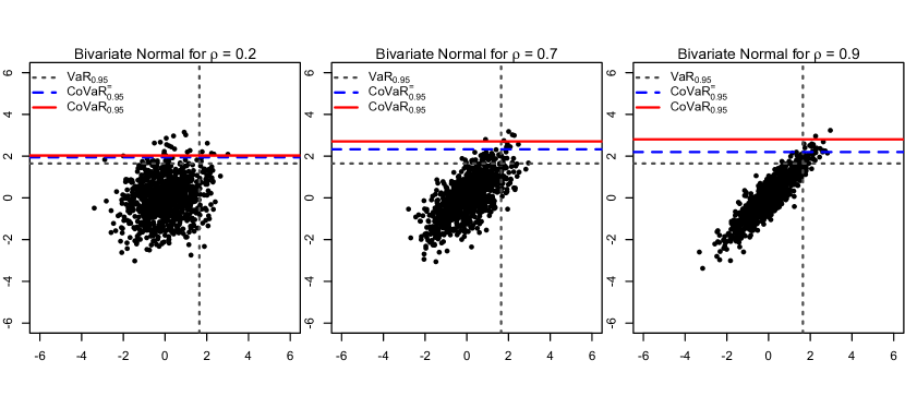
Figure 3: Bivariate normal samples (size $n=2000$) and the joint excess regions in the backtesting experiment for $\alpha=\beta=0.95$.

Risk contribution measures $\operatorname{\Delta CoVaR^{=}}$ and $\operatorname{\Delta^{\mathrm{med}}CoVaR^{=}}$

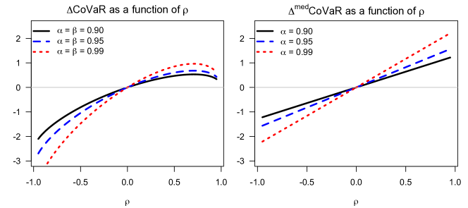
Figure 4: $\operatorname{\Delta CoVaR^{=}_{\alpha}}$ and $\operatorname{\Delta^{\mathrm{med}}CoVaR^{=}_{\alpha}}$ as functions of $\rho$ in the bivariate normal model.

As mentioned in Section 2, [2] aims not at $\operatorname{CoVaR^{=}}$ itself, but at the difference between $\operatorname{CoVaR^{=}}$ and some characteristic of an unstressed state. The two most common definitions of such a risk contribution measure are $\operatorname{\Delta CoVaR^{=}}$ and $\operatorname{\Delta^{\mathrm{med}}CoVaR^{=}}$ (see (3) and (4)). In the bivariate normal case one has $\operatorname{VaR}_{\beta}(Y)=\mu_{Y}+\sigma_{Y}\Phi^{-1}(\beta)$, so that (13) yields

$$\operatorname{\Delta CoVaR^{=}_{\alpha,\beta}}(Y)=\sigma_{Y}\left(\Phi^{-1}\ (\alpha)\rho+\Phi^{-1}(\beta)\left(\sqrt{1-\rho^{2}}-1\right)\right).$$

For $\alpha=\beta$ this simplifies to $\operatorname{\Delta CoVaR^{=}_{\alpha}}(Y)=\sigma_{Y}\Phi^{-1}(\alpha)\left({\rho+\sqrt{1-\rho^{2}}-1}\right)$. Regardless of $\alpha$ and $\beta$, $\operatorname{\Delta CoVaR^{=}}$ inherits the non-monotonicity in $\rho$ from $\operatorname{CoVaR^{=}}$. An illustration to this issue is given in Figure 4, which shows plots of $\operatorname{\Delta CoVaR^{=}}$ and $\operatorname{\Delta^{\mathrm{med}}CoVaR^{=}}$ as functions of $\rho$ for $\alpha=\beta$.

At a first glance, $\operatorname{\Delta^{\mathrm{med}}CoVaR^{=}}$ seems to be an improvement because it is increasing in $\rho$. In fact, $\operatorname{\Delta^{\mathrm{med}}CoVaR^{=}}$ is even linear here. Due to $\operatorname{med}(X)=\mu_{X}$, (12) yields $F_{Y|X=\operatorname{med}(X)}^{\leftarrow}(\beta)=\mu_{Y}+\sigma_{Y}\sqrt{1-\rho^{2}}\Phi^{-1}(\beta)$. Applying (13), one obtains that

$$\operatorname{\Delta^{\mathrm{med}}CoVaR^{=}_{\alpha,\beta}}(Y)$$

$$=\mu_{Y}+\sigma_{Y}\left(\Phi^{-1}(\alpha)\rho+\Phi^{-1}(\beta)\sqrt{1-\rho^{2}}\right)-\left({\mu_{Y}+\sigma_{Y}\Phi^{-1}(\beta)\sqrt{1-\rho^{2}}}\right)$$

$$=\sigma_{Y}\Phi^{-1}(\alpha)\rho.$$ (17)

Thus, in the bivariate normal model, $\operatorname{\Delta^{\mathrm{med}}CoVaR^{=}_{\alpha,\beta}}(Y|X)$ is linear with positive slope that depends on $\rho$ and $\alpha$, but not on $\beta$. In view of the linear structure (12) of the bivariate Gaussian model, this even appears reasonable. However, examples in Sections 4.2 and 4.3 show that $\operatorname{\Delta^{\mathrm{med}}CoVaR^{=}}$ is not a monotonic function of dependence parameters in other models. Thus the applicability of $\operatorname{\Delta^{\mathrm{med}}CoVaR^{=}}$ is restricted to linear models of type (12), where it is superfluous because it carries quite the same information as the correlation parameter $\rho$ or the linear regression parameter from the classical Capital Asset Pricing Model (the so-called CAPM-$\beta$), which is equal to $\rho\sigma_{Y}/\sigma_{X}$ in the present setting.

Extension from $\operatorname{CoVaR}$ to $\operatorname{CoES}$

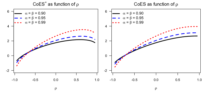
Figure 5: $\operatorname{CoES_{\alpha}^{=}}(Y|X)$ and $\operatorname{CoES_{\alpha}}(Y|X)$ in the bivariate normal model as functions of $\rho$.

Due to Corollary 3.10(a) we already know that $\operatorname{CoES_{\alpha,\beta}}$ is increasing in $\rho$ for all $\alpha$ and $\beta$. The special case $\alpha=\beta$ is illustrated in Figure 5, which shows that $\operatorname{CoES^{=}}$ is not increasing in $\rho$. Due to the light tail of the normal distribution, these plots are similar to those of $\operatorname{CoVaR}$ and $\operatorname{CoVaR^{=}}$ in Figure 1. A closer look at (2) confirms that the non-monotonicity of $\operatorname{CoES^{=}}$ in $\rho$ is inherited from $\operatorname{CoVaR^{=}}$. Thus the best possible extension to Conditional Expected Shortfall based on $\operatorname{CoVaR^{=}}$ still fails to reflect dependence properly.

4.2 Bivariate $t$ distribution

The next example we consider is the bivariate $t$ distribution, which is elliptical, but heavy-tailed. The comparison follows the same scheme as in the previous section. A bivariate $t$ distributed random vector with $\nu>0$ degrees of freedom (bivariate $t(\nu)$) can be obtained as follows:

$$(X,Y):=(\mu_{X},\mu_{Y})+\sqrt{\frac{\nu}{W}}\left({\widetilde{X},\widetilde{Y}}\right),$$

where $(\widetilde{X},\widetilde{Y})\sim\mathcal{N}(0,\Sigma)$ and $W\sim\chi^{2}(\nu)$, independent of $(\widetilde{X},\widetilde{Y})$. The parameters $\mu_{X},\mu_{Y}\in\mathbb{R}$ specify the location of $(X,Y)$. For simplicity, we consider a centred model with $\mu_{X}=\mu_{Y}=0$.

It is well known that the bivariate $t$ distribution is elliptical with ellipticity matrix $\Sigma$. The corresponding sample clouds have an elliptical shape (cf. Figure 8). The second moments of $X$ and $Y$ are finite for $\nu>2$, and in this case the correlation between $X$ and $Y$ is equal to $\rho$. The role of $\rho$ is the same as for all elliptical models: larger values of $\rho$ increase association between large values of $X$ and $Y$. Analytic expressions for $\operatorname{CoVaR^{=}}$ or $\operatorname{CoVaR}$ are not feasible in this model, so that computations have to be carried out numerically.

Monotonicity in $\rho$

The behaviour of $\operatorname{CoVaR^{=}}$ and $\operatorname{CoVaR}$ as functions of the correlation parameter $\rho$ is shown in Figure 6. Similarly to the Gaussian case, $\operatorname{CoVaR}$ is increasing in $\rho$ due to Theorem 3.6(a), whereas $\operatorname{CoVaR^{=}}$ is not. Moreover, the relative distance between $\operatorname{CoVaR^{=}}$ and $\operatorname{CoVaR}$ (as it could be quantified by the ratio $\operatorname{CoVaR}/\operatorname{CoVaR^{=}}$) is larger than in the Gaussian case. A possible explanation to this effect could be the heavy tail of the $t(3)$ distribution.

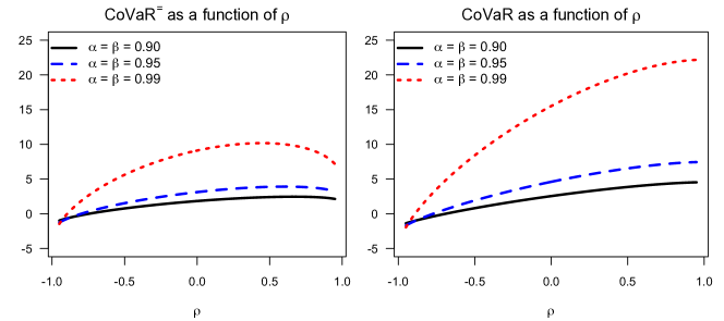
Figure 6: Bivariate $t(3)$ distribution: $\operatorname{CoVaR_{\alpha}^{=}}$ and $\operatorname{CoVaR_{\alpha}}$ as functions of the correlation parameter $\rho$.

Normalized values of $\operatorname{CoVaR}$ and $\operatorname{CoVaR^{=}}$

Figure 7 shows the ratios $\operatorname{CoVaR_{\alpha}^{=}}(Y|X)/\operatorname{VaR}_{\alpha}(Y)$ and $\operatorname{CoVaR_{\alpha}}(Y|X)/\operatorname{VaR}_{\alpha}(X)$ as functions of $\alpha$ for selected values of $\rho$. This comparison is analogous to Figure 2 in the Gaussian case. Similarly to the Gaussian case, the ordering of $\operatorname{CoVaR_{\alpha}^{=}}/\operatorname{VaR}_{\alpha}$ with respect to the dependence parameter $\rho$ or $\theta$ is inconsistent, whereas the ratios $\operatorname{CoVaR_{\alpha}}/\operatorname{VaR}_{\alpha}$ are ordered correctly for all $\alpha$: the line for the largest $\rho$ is entirely above the line for the second largest $\rho$, etc. In contrast to the Gaussian case, these ratios are increasing in $\alpha$. This could be explained by the heavy tail of the $t(3)$ distribution or by the positive tail dependence in the bivariate $t$ model.

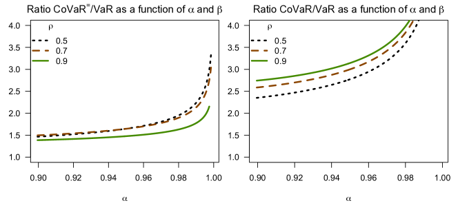
Figure 7: Bivariate $t(3)$ distribution with $\mu_{Y}=0$: Ordering of the ratios $\operatorname{CoVaR_{\alpha}^{=}}(Y|X)/\operatorname{VaR}_{\alpha}(Y)$ and $\operatorname{CoVaR_{\alpha}}(Y|X)/\operatorname{VaR}_{\alpha}(Y)$ for different $\alpha$.

Backtesting and violation rates

The backtesting study was implemented analogously to the bivariate Gaussian example. The results are shown in Table 2, and they go in line with those from the Gaussian case. While $\operatorname{CoVaR}$ – again, by construction – has a violation rate close to $1-\beta$, the violation rates of $\operatorname{CoVaR^{=}}$ are significantly higher and increase in $\rho$. Going up to $36\%$ for $\rho=0.9$, the violation rates for $\operatorname{CoVaR}$ are even higher than in the Gaussian model.

	$\rho=0$	$\rho=0.2$	$\rho=0.5$	$\rho=0.7$	$\rho=0.9$
$\operatorname{CoVaR}^{=}_{0.95,0.95}(Y|X)$	0.1017	0.1213	0.1659	0.2202	0.3638
$\operatorname{CoVaR}^{=}_{0.99,0.99}(Y|X)$	0.0358	0.0433	0.0643	0.0939	0.1909
$\operatorname{CoVaR}^{=}_{0.95,0.99}(Y|X)$	0.0341	0.0429	0.0640	0.0944	0.1954
$\operatorname{CoVaR}^{=}_{0.99,0.95}(Y|X)$	0.1036	0.1229	0.1658	0.2184	0.3546
$\operatorname{CoVaR}_{0.95,0.95}(Y|X)$	0.0497	0.0500	0.0499	0.0506	0.0504
$\operatorname{CoVaR}_{0.99,0.99}(Y|X)$	0.0103	0.0099	0.0104	0.0105	0.0103
$\operatorname{CoVaR}_{0.95,0.99}(Y|X)$	0.0100	0.0099	0.0100	0.0102	0.0101
$\operatorname{CoVaR}_{0.99,0.95}(Y|X)$	0.0501	0.0493	0.0499	0.0508	0.0507

Table 2: Violation rates in the bivariate $t(3)$ case. Monte Carlo backtesting with $n=10^{7}$ and $\alpha,\beta\in\{0.95,0.99\}$.

The corresponding sample plots with lines marking $\operatorname{VaR}_{\alpha}(X)$, $\operatorname{CoVaR_{\alpha}^{=}}(Y|X)$, and $\operatorname{CoVaR_{\alpha}}(Y|X)$ are shown in Figure 8. Similarly to Figure 3, these graphics demonstrate how increasing dependence parameter $\rho$ changes the shape of the corresponding sample clouds and increases the numbers of joint excesses.

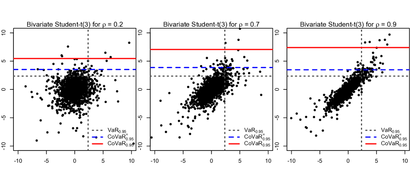
Figure 8: Bivariate $t(3)$ samples (size $n=2000$) and the joint excess regions in the backtesting experiment for $\alpha=\beta=0.95$.

Risk contribution measures $\operatorname{\Delta CoVaR^{=}}$ and $\operatorname{\Delta^{\mathrm{med}}CoVaR^{=}}$

The comparison of $\operatorname{\Delta CoVaR^{=}}$ and $\operatorname{\Delta^{\mathrm{med}}CoVaR^{=}}$ is shown in Figure 9. The graphics demonstrate clearly how these $\operatorname{CoVaR^{=}}$ based risk contribution measures inherit the inconsistency of $\operatorname{CoVaR^{=}}$. Both $\operatorname{\Delta CoVaR^{=}}$ and $\operatorname{\Delta^{\mathrm{med}}CoVaR^{=}}$ fail to be increasing with respect to the dependence parameter $\rho$, and the shapes of the corresponding curves are similar to those of $\operatorname{CoVaR^{=}}$ in Figure 6. Although $\operatorname{\Delta^{\mathrm{med}}CoVaR^{=}}$ is slightly better behaved than $\operatorname{\Delta CoVaR^{=}}$, it is still strongly inconsistent with respect to $\rho$. In particular, this example demonstrates that the monotonicity of $\operatorname{\Delta^{\mathrm{med}}CoVaR^{=}}$ with respect to $\rho$ in the Gaussian case is a special property of the bivariate Gaussian model, so that the advantage of $\operatorname{\Delta^{\mathrm{med}}CoVaR^{=}}$ over $\operatorname{\Delta CoVaR^{=}}$ is quite limited.

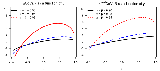
Figure 9: $\operatorname{\Delta CoVaR^{=}_{\alpha}}$ and $\operatorname{\Delta^{\mathrm{med}}CoVaR^{=}_{\alpha}}$ as functions of $\rho$ in the bivariate $t(3)$ model.

Extension from $\operatorname{CoVaR}$ to $\operatorname{CoES}$

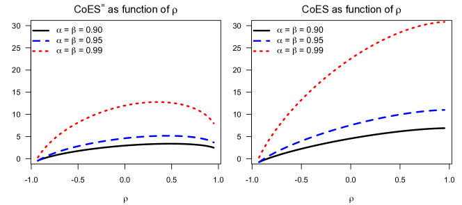
Figure 10: $\operatorname{CoES_{\alpha}^{=}}(Y|X)$ and $\operatorname{CoES_{\alpha}}(Y|X)$ in the bivariate $t(3)$ model as functions of $\rho$.

The comparison of $\operatorname{CoES}$ vs. $\operatorname{CoES^{=}}$ is shown in Figure 10. The monotonicity or non-monotonicity in $\rho$ is again inherited from $\operatorname{CoVaR}$ or $\operatorname{CoVaR^{=}}$. See also Corollary 3.10(a).

4.3 Gumbel copula with $t$ margins

The last model we consider here is obtained by endowing a bivariate Gumbel copula (cf. (10)) with $t$ margins. Thus it has the same heavy-tailed margins as the previous example, but a different dependence structure. An illustration of the sample clouds generated from this distribution is given in Figure 13.

On the qualitative level, all comparison results obtained in this case are similar to the bivariate $t$ model, so that a brief overview is fully sufficient:

• Corollary 3.8 guarantees that $\operatorname{CoVaR_{\alpha,\beta}}$ is increasing with respect to the dependence parameter $\theta$, whereas $\operatorname{CoVaR_{\alpha,\beta}^{=}}$ fails to be increasing if dependence is at its largest (see Figure 11 for the case $\alpha=\beta$). The strongest decay of $\operatorname{CoVaR^{=}}$ takes place for $\theta\in(1.5,2)$ and slows down for $\theta>2$. On the other hand, $\operatorname{CoVaR_{\alpha}}$ is almost constant for $\theta>2$. It seems that for $\theta>2$ the joint distribution of large values of $(X,Y)$ is almost comonotonic, so that there is no much change after $\theta$ exceeds $2$.

• The ratios $\operatorname{CoVaR_{\alpha}}(Y|X)/\operatorname{VaR}_{\alpha}(Y)$ are ordered correctly with respect to $\theta$, whereas the ratios $\operatorname{CoVaR_{\alpha}^{=}}(Y|X)/\operatorname{VaR}_{\alpha}(Y)$ are not (see Figure 12).

• The violation rates for $\operatorname{CoVaR_{\alpha,\beta}^{=}}$ in a simulated backtesting study are significantly larger than $1-\beta$, going up to $40\%$ for $\alpha=\beta=0.95$ and $\theta=3$ (cf. Table 3 and Figure 13). This is even more than in the bivariate $t$ case.

• Both $\operatorname{\Delta CoVaR^{=}}$ and $\operatorname{\Delta^{\mathrm{med}}CoVaR^{=}}$ fail to be increasing in $\theta$ (Figure 14).

• Again, $\operatorname{CoES}$ is increasing in $\theta$ and $\operatorname{CoES^{=}}$ is not; see Corollary 3.10(a) and Figure 15.

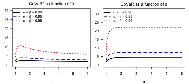
Figure 11: Gumbel copula $t(3)$ margins: $\operatorname{CoVaR_{\alpha}^{=}}(Y|X)$ and $\operatorname{CoVaR_{\alpha}}(Y|X)$ as functions of $\theta$.

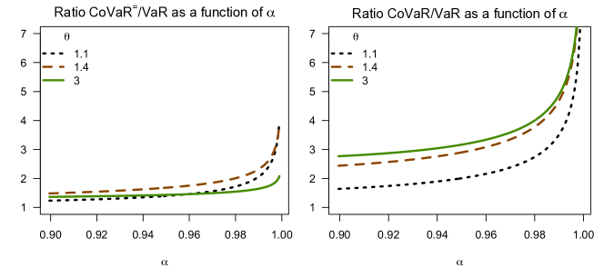
Figure 12: Gumbel copula with $t(3)$ margins: Ordering of the ratios $\operatorname{CoVaR_{\alpha}^{=}}(Y|X)/\operatorname{VaR}_{\alpha}(Y)$ and $\operatorname{CoVaR_{\alpha}}(Y|X)/\operatorname{VaR}_{\alpha}(Y)$ for different $\alpha$.

	$\theta=1$	$\theta=1.1$	$\theta=1.2$	$\theta=1.5$	$\theta=2$	$\theta=3$
$\operatorname{CoVaR}^{=}_{0.95,0.95}(Y|X)$	0.0498	0.0982	0.1282	0.1911	0.2771	0.4090
$\operatorname{CoVaR}^{=}_{0.99,0.99}(Y|X)$	0.0101	0.0346	0.0461	0.0752	0.1321	0.2423
$\operatorname{CoVaR}^{=}_{0.95,0.99}(Y|X)$	0.0098	0.0309	0.0434	0.0754	0.1319	0.2450
$\operatorname{CoVaR}^{=}_{0.99,0.95}(Y|X)$	0.0500	0.1050	0.1335	0.1916	0.2745	0.4043
$\operatorname{CoVaR}_{0.95,0.95}(Y|X)$	0.0498	0.0494	0.0503	0.0498	0.0501	0.0502
$\operatorname{CoVaR}_{0.99,0.99}(Y|X)$	0.0101	0.0099	0.0101	0.0102	0.0100	0.0097
$\operatorname{CoVaR}_{0.95,0.99}(Y|X)$	0.0098	0.0099	0.0100	0.0099	0.0100	0.0098
$\operatorname{CoVaR}_{0.99,0.95}(Y|X)$	0.0500	0.0497	0.0499	0.0492	0.0503	0.0492

Table 3: Violation rates for the Gumbel copula with $t(3)$ margins: Monte Carlo backtesting with $n=10^{7}$ and $\alpha,\beta\in\{0.95,0.99\}$.

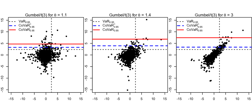
Figure 13: Gumbel copula with $t(3)$ margins: simulated samples (size $n=2000$) and the joint excess regions in the backtesting experiment for $\alpha=\beta=0.95$.

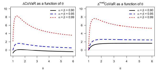
Figure 14: Gumbel copula with $t(3)$ margins: $\operatorname{\Delta CoVaR^{=}_{\alpha}}$ and $\operatorname{\Delta^{\mathrm{med}}CoVaR^{=}_{\alpha}}$ as functions of $\theta$.

Figure 15: Gumbel copula with $t(3)$ margins: $\operatorname{CoES_{\alpha}^{=}}(Y|X)$ and $\operatorname{CoES_{\alpha}}(Y|X)$ as functions of $\theta$.

5 Conclusions

The present paper demonstrates that the alternative definition of Conditional Value-at-Risk proposed in [14, 20] (here $\operatorname{CoVaR}$) gives a much more consistent response to dependence than the original definition used in [2, 3, 4] (here $\operatorname{CoVaR^{=}}$).

The general results in Section 3 show that the monotonicity of $\operatorname{CoVaR_{\alpha,\beta}}(Y|X)$ with respect to dependence parameters is related to the concordance ordering of bivariate distributions or copulas. This gives the notion of $\operatorname{CoVaR}$ based on the stress scenario $\{X\geq\operatorname{VaR}_{\alpha}(X)\}$ a solid mathematical fundament. On the other hand, comparative studies in Section 4 show that conditioning on $\{X=\operatorname{VaR}_{\alpha}(X)\}$ makes $\operatorname{CoVaR^{=}}$ and its derivatives unable to detect systemic risk where it is most pronounced. Related counterexamples include several popular models, in particular the very basic bivariate normal case.

Based on these results, we claim that, if Conditional Value-at-Risk of an institution (or system) $Y$ related to a stress scenario for another institution $X$ should enter financial regulation, then it should use conditioning on $\{X\geq\operatorname{VaR}_{\alpha}(X)\}$. This kind of stress scenario has a much more meaningful practical interpretation than the highly selective and over-optimistic scenario $\{X=\operatorname{VaR}_{\alpha}(X)\}$. Conditioning on $\{X\geq\operatorname{VaR}_{\alpha}(X)\}$ also makes $\operatorname{CoVaR}$ more similar to the systemic risk measures proposed in [15, 1, 29, 16].

The question how to define risk contribution measures based on stress events to the financial system is currently open. Besides $\operatorname{CoVaR}$, $\operatorname{CoES}$ with proper conditioning may also be an option. The advantage of $\operatorname{CoES}$ over $\operatorname{CoVaR}$ is its coherency. In the case $\operatorname{VaR}$ vs. $\operatorname{ES}$, this point has gained new interest from the regulators [7, 13].

In some sense, $\operatorname{CoVaR^{=}}$ repeats two times the design error that is responsible for the non-coherency of $\operatorname{VaR}$. In the first step, it follows the $\operatorname{VaR}$ paradigm and thus favours a single conditional quantile of $Y$ over an average of such quantiles. In the second step, it favours the most benign outcome of $X$ in a state of stress over considering the full range of possible values in this case. Financial regulation based on $\operatorname{CoVaR^{=}}$ has a strong potential to introduce additional instability, to set wrong incentives, and to create opportunities for regulatory arbitrage.

Another argument supporting $\operatorname{CoES}$ is that it is particularly suitable for stress testing. In a system with several factors $X_{1},\ldots,X_{d}$, the numbers $\operatorname{CoES}_{\alpha_{i},\beta}(Y|X_{i})$ describe the influence of the different $X_{i}$ on $Y$. Assigning relative weights $w_{i}$ to the scenarios $X_{i}\geq\operatorname{VaR}_{\alpha_{i}}(X_{i})$ and taking the weighted sum

$$\sum_{i=1}^{d}w_{i}\operatorname{CoES}_{\alpha_{i},\beta}(Y|X_{i}),$$ (18)

one always obtains a sub-additive risk measure. If the weights $w_{i}$ sum up to $1$, the resulting risk measure is coherent in the sense of [5]. The choice of the weights $w_{i}$ or of the confidence levels $\alpha_{i}$ may change over time, incorporating the newest information about the health of the institutions $X_{1},\ldots,X_{d}$.

To make the weighted risk measure (18) even more meaningful, one could modify it by implementing not only the single risk factor excesses $X_{i}\geq\operatorname{VaR}_{\alpha_{i}}(X_{i})$, but also the joint ones. Consistent choice of the corresponding weights can be derived by methods presented in [23]. A detailed discussion of this goes beyond the scope of the present paper and would also require additional mathematical research.

Motivated by the recent financial crisis and the following discussions on appropriate reforms in financial regulation, systemic risk measurement has become a vivid topic in economics and econometrics. Our results show that some important contributions are also to be made in related mathematical fields, including probability and statistics. In particular, the dependence consistency or, say, dependence coherency of systemic risk indicators is a novel problem area that needs further study. The present paper provides first examples and counter-examples for compatibility of systemic risk indicators with the concordance order. The questions for general characterizations or representations of functionals with this property are currently open.

In addition to dependence consistency, implementation of systemic risk measures in practice obviously needs estimation methods. The estimation of $\operatorname{CoVaR}$ in GARCH models is discussed in [14]. As non-parametric estimation of rare events would needs a lot of data, methods from Extreme Value Theory may be used to extrapolate the rear events from a larger number of data points. A similar approach for conditional default probabilities is pursued in [29].

References

- Acharya et al. [2010] V. V. Acharya, L. H. Pedersen, T. Philippon, and M. Richardson. Measuring systemic risk. Preprint, 2010. URL http://papers.ssrn.com/abstract˙id=1573171.
- Adrian and Brunnermeier [2008] T. Adrian and M. Brunnermeier. Covar. Preprint, 2008. URL http://citeseerx.ist.psu.edu/viewdoc/download?doi=10.1.1.140.7052&rep=r%ep1&type=pdf.
- Adrian and Brunnermeier [2009] T. Adrian and M. Brunnermeier. Covar. Preprint, 2009. URL http://papers.ssrn.com/sol3/papers.cfm?abstract˙id=1269446.
- Adrian and Brunnermeier [2010] T. Adrian and M. Brunnermeier. Covar. Preprint, 2010. URL http://www.princeton.edu/~markus/research/papers/CoVaR.
- Artzner et al. [1999] P. Artzner, F. Delbaen, J.-M. Eber, and D. Heath. Coherent measures of risk. Math. Finance, 9(3):203–228, 1999. ISSN 0960-1627. URL http://dx.doi.org/10.1111/1467-9965.00068.
- Balkema and Embrechts [2007] G. Balkema and P. Embrechts. High Risk Scenarios and Extremes. Zurich Lectures in Advanced Mathematics. European Mathematical Society (EMS), Zürich, 2007. ISBN 978-3-03719-035-7.
- Basel Committee on Banking Supervision [2012] Basel Committee on Banking Supervision. Fundamental review of the trading book. Consultative document, Bank for International Settlements (BIS), May 2012. URL http://www.bis.org/publ/bcbs219.htm.
- Boss et al. [2004] M. Boss, H. Elsinger, M. Summer, and S. Thurner 4. Network topology of the interbank market. Quantitative Finance, 4(6):677–684, 2004. URL http://www.tandfonline.com/doi/abs/10.1080/14697680400020325.
- Cambanis and Simons [1982] S. Cambanis and G. Simons. Probability and expectation inequalities. Probability Theory and Related Fields, 59:1–25, 1982. ISSN 0178-8051. URL http://dx.doi.org/10.1007/BF00575522. 10.1007/BF00575522.
- Choi and Douady [2012] Y. Choi and R. Douady. Financial crisis dynamics: attempt to define a market instability indicator. Quantitative Finance, 12(9):1351–1365, 2012. URL http://www.tandfonline.com/doi/abs/10.1080/14697688.2011.627880.
- Cont et al. [2012] R. Cont, A. Moussa, and E. B. e Santos. Network structure and systemic risk in banking systems. Preprint, 2012. URL http://papers.ssrn.com/sol3/papers.cfm?abstract˙id=1733528.
- Embrechts and Hofert [2010] P. Embrechts and M. Hofert. A note on generalized inverses. Preprint, 2010. URL http://www.math.ethz.ch/~baltes/ftp/inverses˙PE˙MH.pdf.
- Gauthier et al. [2012] C. Gauthier, A. Lehar, and M. Souissi. Macroprudential capital requirements and systemic risk. Journal of Financial Intermediation, 2012. ISSN 1042-9573. URL http://www.sciencedirect.com/science/article/pii/S104295731200006X.
- Girardi and Ergün [2012] G. Girardi and T. Ergün. Systemic risk measurement: Multivariate garch estimation of covar. Preprint, 2012. URL http://papers.ssrn.com/sol3/papers.cfm?abstract˙id=1783958.
- Goodhart and Segoviano [2008] C. Goodhart and M. A. Segoviano. Banking stability measures. IMF working paper, 2008. URL http://www.bcentral.cl/eng/conferences-seminars/annual-conferences/2008%/papers/9%20Segoviano˙paper.pdf.
- Huang et al. [2011] X. Huang, H. Zhou, and H. Zhu. Systemic risk contributions. Journal of Financial Services Research, pages 1–29, 2011. ISSN 0920-8550. URL http://dx.doi.org/10.1007/s10693-011-0117-8. 10.1007/s10693-011-0117-8.
- Ibragimov and Walden [2007] R. Ibragimov and J. Walden. The limits of diversification when losses may be large. Journal of Banking & Finance, 31(8):2551 – 2569, 2007. ISSN 0378-4266. URL http://www.sciencedirect.com/science/article/pii/S037842660700043X.
- Jaeger-Ambrozewicz [2010] M. Jaeger-Ambrozewicz. Systemic risk and covar in a gaussian setting. preprint, 2010. URL http://papers.ssrn.com/sol3/papers.cfm?abstract˙id=1675435.
- Joe [1997] H. Joe. Multivariate Models and Dependence Concepts, volume 73 of Monographs on Statistics and Applied Probability. Chapman & Hall, London, 1997. ISBN 0-412-07331-5.
- Klyman [2011] J. Klyman. Systemic Risk Measures: DistVaR and Other “Too Big To Fail” Risk Measures. Doctoral thesis, Department of Operations Research and Financial Engineering, Princeton University, Princeton, New Jersey, 2011. URL http://gradworks.umi.com/34/52/3452603.html.
- McNeil et al. [2005] A. McNeil, R. Frey, and P. Embrechts. Quantitative Risk Management: Concepts, Techniques and Tools. Princeton University Press, 2005.
- Müller and Stoyan [2002] A. Müller and D. Stoyan. Comparison Methods for Stochastic Models and Risks. Wiley Series in Probability and Statistics. John Wiley & Sons Ltd., Chichester, 2002. ISBN 0-471-49446-1.
- Rebonato [2010] R. Rebonato. Coherent Stress Testing: A Bayesian Approach to the Analysis of Financial Stress. Wiley, UK, 2010.
- Sklar [1959] A. Sklar. Fonctions de répartition á n dimensions et leurs margins. Publ. Inst. Statist. Univ. Paris, 8:229–231, 1959.
- Staum [2012] J. Staum. Systemic risk components and deposit insurance premia. Quantitative Finance, 12(4):651–662, 2012. URL http://www.tandfonline.com/doi/abs/10.1080/14697688.2012.664942.
- Tarashev et al. [2010] N. Tarashev, C. Borio, and K. Tsatsaronis. Attributing systemic risk to individual institutions. Working paper, Bank for International Settlements (BIS), May 2010. URL http://www.bis.org/publ/work308.htm.
- Tong [1990] Y. L. Tong. The multivariate normal distribution. Springer Series in Statistics. Springer-Verlag, New York, 1990. ISBN 0-387-97062-2.
- Wei and Hu [2002] G. Wei and T. Hu. Supermodular dependence ordering on a class of multivariate copulas. Stat. Probab. Lett., 57(4):375–385, 2002. ISSN 0167-7152. URL http://dx.doi.org/10.1016/S0167-7152(02)00094-9.
- Zhou [2010] C. Zhou. Are banks too big to fail? Measuring systemic importance of financial institutions. International Journal of Central Banking, 6(4):205–250, 2010. URL http://www.ijcb.org/journal/ijcb10q4a10.pdf.