Persistent currents in a bosonic mixture in the ring geometry

Abstract

In this paper we analyze the possibility of persistent currents of a two-species bosonic mixture in the one-dimensional ring geometry. We extend the arguments used by Bloch Bloch73 to obtain a criterion for the stability of persistent currents for the two-species system. If the mass ratio of the two species is a rational number, persistent currents can be stable at multiples of a certain total angular momenta. We show that the Bloch criterion can also be viewed as a Landau criterion involving the elementary excitations of the system. Our analysis reveals that persistent currents at higher angular momenta are more stable for the two-species system than previously thought.

I introduction

The hallmark of superfluidity is the possibility of dissipationless flow in situations where the flow of a normal fluid would degrade as a result of viscosity. The textbook example of this is the flow of a superfluid through a narrow capillary Wilks70 . According to the Landau criterion Lifshitz80 , the superfluid component flows without dissipation provided the superfluid velocity does not exceed some critical value. In this situation, the normal component remains locked to the walls of the capillary whereas the superfluid component, carrying zero entropy, flows as if the walls of the capillary behaved as a perfectly smooth conduit. If the capillary is now bent into a torus, one can imagine that a flow, once established, could persist indefinitely.

The conditions under which persistent currents can occur for a bosonic mixture in the ring geometry is the subject of this paper. The usual analysis Lifshitz80 leading to the Landau criterion is not obviously applicable since one cannot invoke Galilean invariance for this closed system. However, for a system having a single component, Bloch Bloch73 presented general arguments based on an analysis of the quantum mechanical many-body wave function which provided a criterion for persistent currents. He considered an idealized one-dimensional ring of radius $R$ in which the particles interact via an arbitrary pair-wise interaction. Since the total angular momentum commutes with the Hamiltonian of the system, the stationary states have energies $E_{\alpha}(L)$ which are functions of the angular momentum quantum number $L$; all other quantum numbers are subsumed in the index $\alpha$. Bloch showed that these energy eigenvalues take the form

$$E_{\alpha}(L)=\frac{L^{2}}{2M_{\rm T}R^{2}}+e_{\alpha}(L)$$ (1)

where $M_{\rm T}=NM$ is the total mass of the system containing $N$ particles of mass $M$. The first term on the right hand side of Eq. (1) is interpreted as the kinetic energy of a rigid ring rotating with angular velocity $\Omega=L/M_{T}R^{2}$. The second term, $e_{\alpha}(L)$, corresponds to internal excitations of the system; it has the periodicity property

$$e_{\alpha}(L+N\hbar)=e_{\alpha}(L).$$ (2)

This implies that the system can find itself in the same internal state for angular momenta that differ from each other by multiples of $N\hbar$. In addition, $e_{\alpha}(L)$ has the inversion property

$$e_{\alpha}(-L)=e_{\alpha}(L),$$ (3)

which reflects the fact that the energy does not depend on the sense of the angular momentum.

The state with the lowest energy for a given $L$ will be given the label $\alpha=0$. In the noninteracting limit, $e_{0}(L)$ has a local minimum at $L=0$ Bloch73 ; one expects this property to persist with repulsive interactions. The periodicity of this function then implies that $E_{0}(L)$ can exhibit local minima at certain multiples of $N\hbar$. If and when such minima occur, Bloch argued that the system is capable of sustaining persistent currents. Conversely, if $E_{0}(L)$ is not at a local minimum, nonidealities will induce transitions which change the angular momentum and hence the flow of the superfluid around the ring.

In Sec. II, we extend Bloch’s analysis to a two-species gas containing $N_{A}$ particles of type $A$ and $N_{B}$ particles of type $B$. Here the term “species” can refer either to different kinds of atoms or to atoms distinguished by their hyperfine states. When the masses of the two species are different, we find that the energy can still be written in the form of Eq. (1) but in general, $e_{0}(L)$ is no longer a periodic function of $L$. However, if the masses are equal, $e_{0}(L)$ is found to have the same periodicity as for the single-species case with $N=N_{A}+N_{B}$. In the case that the mass ratio $M_{A}/M_{B}$ is a rational number, $e_{0}(L)$ remains a periodic function of $L$ but with a periodicity that differs from $N\hbar$. For these special cases, Bloch’s arguments for the possibility of persistent currents goes through as for the single-species case. For arbitrary mass ratios, $E_{0}(L)$ may still exhibit a local minimum at some finite value of $L$ but there is no general argument which can be used to determine where such a local minimum might occur.

We go on to show that Bloch’s criterion for persistent currents can be phrased in terms of the more familiar Landau criterion. For $M_{A}=M_{B}$, $e_{0}(L)$ is periodic and a Landau criterion can be formulated at the discrete set of angular momenta $L=L_{n}=nN\hbar$, with $n$ an integer, where the system can be taken to be in its internal ground state. The Landau criterion then imposes a constraint on the spectrum of the elementary excitations with angular momentum $m\hbar$ and energy $\varepsilon(m)$. In Sec. III, these excitation energies are determined for the two-species system in the Bogoliubov approximation. In general there are two Bogoliubov modes which are usually phonon-like at long wavelengths. For the case $M_{A}=M_{B}$, the Landau criterion then suggests that persistent currents may be stable for certain values of $n$. However, if the interaction parameters satisfy a certain relation (given in Sec. III), one of the Bogoliubov modes has a particle-like dispersion and the Landau criterion leads to the conclusion that persistent currents are unstable for all $n$.

The above conclusion was arrived at earlier by Smyrnakis et al. Smyrnakis09 based on an analysis of the mean-field Gross-Pitaevskii (GP) energy functional for the two-species system. With the assumption that all interaction parameters are equal, these authors determine $E_{0}(L)$ by minimizing the GP energy functional subject to the constraint that the average angular momentum of the system is $L$. Although persistent currents are destabilized at $L=L_{n}$, the authors find that $E_{0}(L)$ can exhibit local minima at non-integral values of $l=L/N\hbar$. In particular, they show that persistent currents are stable at $l=x_{A}=N_{A}/(N_{A}+N_{B})$, provided the interactions are sufficiently strong. Furthermore, their analysis leads to the conclusion that persistent currents are unstable for $l>1$ even when the concentration of the minority component is arbitrarily small. This latter conclusion seems at odds with what one might expect in the pure single-species limit ($x_{B}\to 0$).

In Sec. IV, we present the analysis of the GP energy functional in somewhat more detail than was provided by Smyrnakis et al. Smyrnakis09 This analysis essentially confirms all of their analytical results, however, we find that the information regarding the behaviour of $e_{0}(L)$ in the vicinity of $L=N_{A}\hbar$ is not sufficient to establish whether or not persistent currents are actually stable. In fact, a more global analysis of $e_{0}(L)$ shows that persistent currents can exist when $l>1$. Our work also clarifies how the single-species results are recovered in the $x_{B}\to 0$ limit.

II Bloch’s criterion for persistent currents in a two-species gas

In this section we extend Bloch’s analysis to a two-species system consisting of $N_{A}$ particles of type $A$ and $N_{B}$ particles of type $B$. The masses of the particles are $M_{A}$ and $M_{B}$. In addition, we assume an idealized one-dimensional ring geometry. The Hamiltonian $H$ for this system is taken to be

$${H}=\sum\limits_{i=1}^{N_{A}}\frac{\hat{l}_{i}^{2}}{2M_{A}R^{2}}+\sum\limits_{i=N_{A}+1}^{N_{A}+N_{B}}\frac{\hat{l}_{i}^{2}}{2M_{B}R^{2}}+\sum\limits_{i<j}v_{ij}(\theta_{i}-\theta_{j}),$$ (4)

where the angular momentum operator of the $i$-th particle about the centre of the ring is

$$\hat{l}_{i}=\frac{\hbar}{i}\frac{\partial}{\partial\theta_{i}}.$$ (5)

The index $i$ denotes an $A$-type particle for $1\leq i\leq N_{A}$ and a $B$-type particle for $N_{A}+1\leq i\leq N_{A}+N_{B}\equiv N$. The subscripts on the interaction potential $v_{ij}$ allow for the interactions between the particles to be species-dependent. For the pair-wise interactions assumed, the total angular momentum

$$\hat{L}=\sum\limits_{i=1}^{N}\hat{l}_{i}=\sum\limits_{i=1}^{N}\frac{\hbar}{i}\frac{\partial}{\partial\theta_{i}}$$ (6)

commutes with the Hamiltonian. The stationary states $\Psi(\theta_{1},...,\theta_{N})$ of the Hamiltonian can thus be chosen to be simultaneous eigenstates of the total angular momentum.

A suitable basis of states can be constructed from the following product states for noninteracting particles:

$$\Phi(\theta_{1},...,\theta_{N})=\phi_{m_{1}}(\theta_{1})\phi_{m_{2}}(\theta_{2})\cdots\phi_{m_{N}}(\theta_{N}).$$ (7)

Here $m_{i}$ is an integer and

$$\phi_{m}(\theta)=\frac{e^{im\theta}}{\sqrt{2\pi}}.$$ (8)

The wave function in Eq. (7) is an eigenfunction of $\hat{L}$ with eigenvalue $L=\hbar\sum_{i}m_{i}$. It can be written in different ways. One possibility is

$$\Phi(\theta_{1},...,\theta_{N})=(2\pi)^{-N/2}\exp(iNl\Theta)\exp\bigg{[}\frac{i}{N}\sum_{ij}m_{i}(\theta_{i}-\theta_{j})\bigg{]}$$ (9)

where

$$l=\frac{1}{N}\sum_{i=1}^{N}m_{i}$$ (10)

is the angular momentum per particle in units of $\hbar$ and

$$\Theta=\frac{1}{N}\sum_{i=1}^{N}\theta_{i}$$ (11)

is the mean angular coordinate. The above wave function is identical in form to that of a single species system. By construction, the first exponential in Eq. (9) is an eigenfunction of $\hat{L}$ with eigenvalue $L=Nl\hbar$. The second exponential is a function of the coordinate differences $\theta_{i}-\theta_{j}$ and as such is a zero total angular momentum wave function.

Properly symmetrized functions are obtained from Eq. (9) with the application of the symmetrization operator

$$\hat{S}=\hat{S}_{A}\hat{S}_{B}$$ (12)

where

$$\hat{S}_{A}=\frac{1}{N_{A}!}\sum\limits_{P_{A}}\hat{P}_{A}$$ (13)

$$\hat{S}_{B}=\frac{1}{N_{B}!}\sum\limits_{P_{B}}\hat{P}_{B}.$$ (14)

The operator $\hat{P}_{A}$ permutes the coordinates of the $A$ particles, whereas $\hat{P}_{B}$ does the same for $B$ particles. Applying the symmetrization operator to the wave function $\Phi(\theta_{1},...,\theta_{N})$ yields

$$\Phi_{\{m_{i}\}}(\theta_{1},...,\theta_{N})=\exp\left(iNl\Theta\right)\tilde{\chi}_{\{m_{i}\}}(\theta_{1},...,\theta_{N}),$$ (15)

where $\tilde{\chi}_{\{m_{i}\}}$ is a normalized function of the coordinate differences $\theta_{i}-\theta_{j}$. The functions in Eq. (15) provide a basis of properly symmetrized $N$-particle states, with $N=N_{A}+N_{B}$.

The stationary state solutions of $\hat{H}\Psi=E\Psi$ with angular momentum $L$ will be denoted $\Psi_{L\alpha}(\theta_{1},...,\theta_{N})$, where $\alpha$ indicates the rest of the quantum numbers. These states can be expanded in terms of the basis functions Eq. (15) as

$$\Psi_{L\alpha}(\theta_{1},...,\theta_{N})={\sum_{\{m_{i}\}}}^{\prime}C_{L\alpha}(\{m_{i}\})\Phi_{\{m_{i}\}}(\theta_{1},...,\theta_{N})$$

$$\hskip 61.17325pt\equiv\exp\left[iNl\Theta\right]\tilde{\chi}_{L\alpha}(\theta_{1},...,\theta_{N}),$$ (16)

where the prime on the summation implies the restriction $\sum_{i=1}^{N}m_{i}=Nl$. It is clear from the way $\tilde{\chi}_{L\alpha}(\theta_{1},...,\theta_{N})$ is defined that it is a function of the relative angular coordinates $\theta_{i}-\theta_{j}$. Substituting Eq. (II) into the Schrödinger equation for $\Psi_{L\alpha}$, we find that $\tilde{\chi}_{L\alpha}$ satisfies the equation

$$H_{L}\tilde{\chi}_{L\alpha}=\tilde{e}_{\alpha}(L)\tilde{\chi}_{L\alpha},$$ (17)

where

$$H_{L}=H+\frac{L}{NR^{2}}\left(\frac{\hat{L}_{A}}{M_{A}}+\frac{\hat{L}_{B}}{M_{B}}\right)$$ (18)

and

$$\tilde{e}_{\alpha}(L)=E_{\alpha}(L)-\left(\frac{\hbar^{2}l^{2}N_{A}}{2M_{A}R^{2}}+\frac{\hbar^{2}l^{2}N_{B}}{2M_{B}R^{2}}\right)=E_{\alpha}(L)-\frac{L^{2}}{2N^{2}R^{2}}\left(\frac{N_{A}}{M_{A}}+\frac{N_{B}}{M_{B}}\right).$$ (19)

Since $\hat{L}\tilde{\chi}_{L\alpha}=0$, $H_{L}$ in Eq. (17) can be expressed equivalently as

$$H_{L}=H+\frac{L}{NR^{2}}\left(\frac{1}{M_{A}}-\frac{1}{M_{B}}\right)\hat{L}_{A}.$$ (20)

We observe that this Hamiltonian is in general $L$-dependent which has important consequences for $\tilde{e}_{\alpha}(L)$.

Eq. (17) must be solved with appropriate boundary conditions. Since the wave function $\Psi_{L\alpha}$ is required to be single-valued with respect to each of the angular variables, it satisfies

$$\Psi_{L\alpha}(...,\theta_{i}+2\pi,...)=\Psi_{L\alpha}(...,\theta_{i},...).$$ (21)

Eq. (21) then implies

$$\tilde{\chi}_{L\alpha}(...,\theta_{i}+2\pi,...)=\exp\left[-i2\pi l\right]\tilde{\chi}_{L\alpha}(...,\theta_{i},...)$$ (22)

for $i=1,...,N$. From this we see that the boundary conditions are periodic as a function of $L$ with period $N\hbar$. With the basis functions written in the form given in Eq. (9), they are the same boundary conditions that apply in the single-species case. In the $N_{B}=0$ limit, $\tilde{e}_{\alpha}(L)=E_{\alpha}(L)-L^{2}/2M_{T}R^{2}\equiv e_{\alpha}(L)$ with $M_{T}=NM_{A}$. In addition, the Hamiltonian $H_{L}$ reduces to $H$ since $\hat{L}_{A}\to\hat{L}$ and $\hat{L}\tilde{\chi}_{L\alpha}=0$. As a result, $\tilde{\chi}_{L^{\prime}\alpha}$ with $L^{\prime}=L+N\hbar$ satisfies the same Schrödinger equation and boundary conditions as $\tilde{\chi}_{L\alpha}$. This implies that the eigenvalue spectrum for these two functions is identical. As concluded by Bloch Bloch73 , the eigenvalues $e_{\alpha}(L)$ for the single-component system are then periodic functions of $L$ with period $N\hbar$. In particular, the ground state energy is given by

$$E_{0}(L)=\frac{L^{2}}{2NM_{A}R^{2}}+e_{0}(L).$$ (23)

The same considerations apply to the two-species situation for the special case $M_{A}=M_{B}$ since $H_{L}$ in Eq. (20) also reduces to $H$ in this limit and Eq. (23) is still valid. In both of the above situations, the periodicity of the eigenvalues $e_{\alpha}(L)$ means physically that the “internal” excitations can be the same for distinct macroscopic flows whose angular momenta differ by some multiple of $N\hbar$. However, $\tilde{e}_{0}(L)$ is no longer periodic when $M_{A}\neq M_{B}$, since the Hamiltonian $H_{L}$ in Eq. (17) depends explicitly on $L$.

An alternative analysis is provided by writing the wave function in (II) as

$$\Psi_{L\alpha}(\theta_{1},...,\theta_{N})=\exp(iNl\Theta_{\rm cm})\chi_{L\alpha}(\theta_{1},...,\theta_{N}),$$ (24)

where $\Theta_{\rm cm}$ is the ‘centre-of-mass’ angular coordinate defined as

$$\Theta_{\rm cm}=\frac{1}{M_{T}}\sum_{i=i}^{N}M_{i}\theta_{i}$$ (25)

and

$$\chi_{L\alpha}(\theta_{1},...,\theta_{N})=\exp\left[-i\frac{l}{M_{T}}\sum_{ij}^{N}M_{i}(\theta_{i}-\theta_{j})\right]\tilde{\chi}_{L\alpha}(\theta_{1},...,\theta_{N}).$$ (26)

Here and in the following, $M_{i}$ is equal to $M_{A}$ for $i\leq N_{A}$ and $M_{B}$ for $i>N_{A}$; $M_{T}=N_{A}M_{A}+N_{B}M_{B}$ is the total mass. We observe that the exponential in Eq. (24) is still an eigenfunction of $\hat{L}$ with eigenvalue $L$ and that $\chi_{L\alpha}$ is a function of coordinate differences and therefore a zero-angular momentum function. Eq. (24) amounts to a separation of the centre-of-mass motion from the internal degrees of freedom. Indeed, substitution of Eq. (24) into the Schrödinger equation for $\Psi_{L\alpha}$ yields

$$H\chi_{L\alpha}=e_{\alpha}(L)\chi_{L\alpha},$$ (27)

where

$$e_{\alpha}(L)=E_{\alpha}(L)-\frac{L^{2}}{2M_{T}R^{2}}.$$ (28)

Eqs. (27) and (28) suggest that $\chi_{L\alpha}$ and $e_{\alpha}(L)$ can be viewed, respectively, as the “internal” wave function and “internal” excitation energy. The boundary conditions imposed on $\chi_{L\alpha}(\theta_{1},...,\theta_{N})$ can be derived from Eq. (24) and are given by

$$\chi_{L\alpha}(\cdots,\theta_{i}+2\pi,\cdots)=\exp\left(-i2\pi\frac{\nu M_{i}}{M_{T}}\right)\chi_{L\alpha}(\cdots,\theta_{i},\cdots),$$ (29)

where $\nu=Nl$. When $M_{A}=M_{B}=M$, these boundary conditions revert to those of the single-species case where

$$\chi_{L\alpha}(\cdots,\theta_{i}+2\pi,\cdots)=\exp\left(-i2\pi l\right)\chi_{L\alpha}(\cdots,\theta_{i},\cdots).$$ (30)

This, together with Eq. (27) implies that $\chi_{L+N\hbar,\alpha}=\chi_{L\alpha}$ and $e_{\alpha}(L+N\hbar)=e_{\alpha}(L)$. In fact, in this case $e_{\alpha}(L)$ and $\chi_{L\alpha}$ coincide with $\tilde{e}_{n}(L)$ and $\tilde{\chi}_{L\alpha}$, respectively.

When $M_{A}\neq M_{B}$, $e_{\alpha}(L)$ is not in general a periodic function of $L$. However, it can be if the boundary conditions in Eq. (29) remain unaltered when $\nu$ is augmented by some number $\tilde{N}$ (i.e., $L\rightarrow L+\tilde{N}\hbar$) such that

$$\frac{\tilde{N}M_{A}}{M_{\rm T}}=p,$$ (31)

and

$$\frac{\tilde{N}M_{B}}{M_{\rm T}}=q,$$ (32)

where $p$ and $q$ are both integers. This implies that $M_{A}/M_{B}$ must be equal to the rational number $p/q$. The lowest possible value of $\tilde{N}$ is obtained when $p$ and $q$ have no common divisor and is then given by

$$\tilde{N}=pN_{A}+qN_{B}.$$ (33)

With this choice of $\tilde{N}$, $e_{\alpha}(L)$ is a periodic function of $L$ with periodicity $\tilde{N}\hbar$. In this situation, it is possible to impart a definite angular momentum to the two-species system without altering its “internal” state. For two different atomic species, the mass ratio $M_{A}/M_{B}$ is never strictly a rational number and thus $e_{\alpha}(L)$ cannot be strictly periodic. However, if

$$M_{A}/M_{B}\simeq p/q+\delta$$ (34)

where $|\delta|<<p/q$, one would expect $e_{\alpha}(L)$, by continuity, to be quasi-periodic with a periodicity close to $(N_{A}p+N_{B}q)\hbar$. For example, a mixture of ${}^{85}{\rm Rb}$ ($A$) and ${}^{39}{\rm K}$ ($B$) has a mass ratio

$$M_{A}/M_{B}\simeq 2+0.07,$$ (35)

in which case the quasi-periodicity of $e_{\alpha}(L)$ would be $(2N_{A}+N_{B})\hbar$.

In the rest of this section we discuss the close connection between Bloch’s argument on persistent currents and Landau’s criterion for superfluidity. Our analysis mainly concerns the single-species and equal-mass two-species systems, where there is strict periodicity for $e_{\alpha}(L)$. However, it also applies to the two-species system with unequal masses, insofar as it is a good approximation to regard $e_{0}(L)$ as quasi-periodic. According to Bloch, persistent currents can occur at the angular momenta $L_{n}=nN\hbar$, for integral $n$, if $E_{0}(L)$ has a local minimum at $L=L_{n}$. We thus examine the behaviour of $E_{0}(L)$ in the neighbourhood of $L_{n}$. From Eqs. (1) and (2) one has

$$E_{0}(L_{n}+\Delta L) = \frac{(L_{n}+\Delta L)^{2}}{2M_{T}R^{2}}+e_{0}(L_{n}+\Delta L)$$ (36)

$$= \frac{L_{n}^{2}}{2M_{T}R^{2}}+\Omega_{n}\Delta L+E_{0}(\Delta L),$$

where $\Omega_{n}\equiv L_{n}/(M_{\rm T}R^{2})$ is the angular velocity of the centre of mass of the system at $L_{n}$. This expression for the energy is analogous to the expression obtained via a Galilean transformation for a homogeneous system in which an excitation is produced in the rest frame of the superfluid Lifshitz80 . To make this correspondence evident, we define the velocity $v_{n}\equiv L_{n}/M_{T}R$ and write the energy in Eq. (36) as

$$E_{0}(L_{n}+\Delta L)=\frac{1}{2}M_{T}v_{n}^{2}+\left(\frac{\Delta L}{R}\right)v_{n}+E_{0}(\Delta L).$$ (37)

The first term on the right hand side is identified as the kinetic energy of the superfluid moving with velocity $v_{n}$. Likewise, the last term is identified as the energy of a stationary superfluid containing an excitation with “momentum” $\Delta L/R$. It should be noted, however, that the analogy is not complete since for a homogeneous system the superfluid velocity $v_{n}$ can take arbitrary values whereas for the ring geometry the angular momentum is restricted to the discrete values $L_{n}$.

With this correspondence in mind, we take $E_{0}(\Delta L)$ to be the energy of the system with a single quasi-particle excitation with angular momentum $\Delta L=\hbar m$ and energy $\varepsilon(m)$, i.e.,

$$E_{0}(\Delta L)=E_{0}(0)+\varepsilon(m).$$ (38)

We thus have

$$E_{0}(L_{n}+\Delta L)=E_{0}(L_{n})+\varepsilon(m)+\Omega_{n}\hbar m.$$ (39)

The stability of the state with energy $E_{0}(L_{n})$ is then assured if the excitations lead to an increase in energy. In other words, the system will sustain persistent currents at $L_{n}$ for an arbitrary excitation of the system if

$$\varepsilon(m)+\hbar\Omega_{n}m>0$$ (40)

for all $m$. Since $\varepsilon(-m)=\varepsilon(m)$, the left hand side has a minimum for negative values of $m$ and we thus require

$$\Omega_{n}<\left(\frac{\varepsilon(m)}{\hbar|m|}\right)_{\rm{min}}.$$ (41)

We have thus shown that Bloch’s argument for persistent currents in the one-dimensional ring geometry naturally leads to the more familiar Landau criterion for superfluidity. If $\varepsilon(m)$ has a positive curvature as a function of $m$, which precludes a roton-like minimum, the inequality in Eq. (41) can be replaced by

$$\Omega_{n}<\frac{\varepsilon(m=1)}{\hbar}.$$ (42)

It is clear from this expression that the inequality must eventually fail when $n$ exceeds some critical value $n_{\rm cr}$.

III Bogoliubov excitations, dynamic stability and Persistent currents at integer values of angular momentum per particle

The Landau criterion derived in the previous section focuses attention on the elementary excitations of the system. In this section, we obtain these excitations for a two-species gas in a one-dimensional ring geometry in the Bogoliubov approximation. We then apply Eq. (42) to discuss persistent currents at integer values of angular momentum per particle for an equal-mass two-species system.

In the following, we assume that the particles interact via contact interactions with strengths $U_{ss^{\prime}}$, where $s,s^{\prime}=A,B$ specify the species. Using the single-particle basis in Eq. (8), the Hamiltonian in Eq. (4) can be written in the second-quantized form

$$\hat{H} = \sum_{s}\sum_{m}\epsilon_{s}\hat{a}^{\dagger}_{s,m}\hat{a}_{s,m}+\sum_{s,s^{\prime}}\sum_{m,m^{\prime},n}\frac{U_{ss^{\prime}}}{4\pi}\hat{a}^{\dagger}_{s,m}\hat{a}^{\dagger}_{s^{\prime},n-m}\hat{a}_{s^{\prime},m^{\prime}}\hat{a}_{s,n-m^{\prime}},$$ (43)

where $m$ is the angular momentum quantum number and $\epsilon_{s}=\hbar^{2}m^{2}/2M_{s}R^{2}$. Assuming both species to be Bose-condensed in the $m=0$ state, the corresponding Bogoliubov Hamiltonian can be written as

$$\hat{H}_{\rm Bog} = \frac{1}{2}\sum_{s,s^{\prime}}\sqrt{N_{s}N_{s^{\prime}}}g_{ss^{\prime}}+\sum_{s}\sum_{m\neq 0}\left[(\epsilon_{s}+g_{ss})\hat{a}^{\dagger}_{s,m}\hat{a}_{s,m}+\frac{1}{2}g_{ss}\hat{a}^{\dagger}_{s,m}\hat{a}^{\dagger}_{s,-m}+\frac{1}{2}g_{ss}\hat{a}_{s,m}\hat{a}_{s,-m}\right]$$ (44)

$$\hskip 104.79128pt+\sum_{s\neq s^{\prime}}\sum_{m\neq 0}g_{ss^{\prime}}\left[\hat{a}^{\dagger}_{s,m}\hat{a}_{s^{\prime},m}+\frac{1}{2}\hat{a}^{\dagger}_{s,m}\hat{a}^{\dagger}_{s^{\prime},-m}+\frac{1}{2}\hat{a}_{s,m}\hat{a}_{s^{\prime},-m}\right],$$

where $g_{ss^{\prime}}=U_{ss^{\prime}}\sqrt{N_{s}N_{s^{\prime}}}/2\pi$.

The diagonalization of a Hamiltonian similar to Eq. (44) for a three-dimensional system was carried out in Tommasini03 . Here we present a different method of determining the Bogoliubov quasiparticle operators. This is done in three steps. First, we perform a Bogoliubov transformation for each of the species treated individually. The transformation is defined by

$$\hat{a}_{s,m}=u^{(0)}_{s,m}\hat{\beta}_{s,m}-v^{(0)}_{s,m}\hat{\beta}^{\dagger}_{s,-m}$$

$$\hat{a}_{s,-m}=u^{(0)}_{s,m}\hat{\beta}_{s,-m}-v^{(0)}_{s,m}\hat{\beta}^{\dagger}_{s,m},$$ (45)

with

$$\big{(}{u^{(0)}_{s,m}}\big{)}^{2}=\frac{1}{2}\left(\frac{\epsilon_{s}+g_{ss}}{E_{s}}+1\right)=\frac{(E_{s}+\epsilon_{s})^{2}}{4E_{s}\epsilon_{s}},\qquad\big{(}{v^{(0)}_{s,m}}\big{)}^{2}=\frac{1}{2}\left(\frac{\epsilon_{s}+g_{ss}}{E_{s}}-1\right)=\frac{(E_{s}-\epsilon_{s})^{2}}{4E_{s}\epsilon_{s}},$$ (46)

where

$$E_{s}=\sqrt{\epsilon_{s}^{2}+2\epsilon_{s}g_{ss}}.$$ (47)

$E_{s}$ is the Bogoliubov excitation energy for independent components. Substituting Eq. (III) into Eq. (44) and dropping all constant terms, we obtain

$$\hat{H}_{\rm Bog}=\sum_{s}\sum_{m\neq 0}E_{s}\hat{\beta}^{\dagger}_{s,m}\hat{\beta}_{s,m}+\sum_{s\neq s^{\prime}}\sum_{m\neq 0}\tilde{g}\left[\hat{\beta}^{\dagger}_{s,m}\hat{\beta}_{s^{\prime},m}+\frac{1}{2}\hat{\beta}^{\dagger}_{s,m}\hat{\beta}^{\dagger}_{s^{\prime},-m}+\frac{1}{2}\hat{\beta}_{s,m}\hat{\beta}_{s^{\prime},-m}\right],$$ (48)

where $\tilde{g}\equiv\sqrt{\epsilon_{A}\epsilon_{B}/E_{A}E_{B}}g_{AB}$. The second term in this Hamiltonian describes the coupling between the Bogoliubov excitations defined for each of the species. It is convenient to write the Hamiltonian (again to within a constant) in the matrix form

$$\hat{H}_{\rm Bog}=\sum_{m>0}\hat{\bf{\Phi}}^{\dagger}_{m}\mathcal{M}\hat{\bf{\Phi}}_{m},$$ (49)

where

$$\hat{\bf{\Phi}}_{m}\equiv(\hat{\beta}_{A,m}\quad\hat{\beta}^{\dagger}_{A,-m}\quad\hat{\beta}_{B,m}\quad\hat{\beta}^{\dagger}_{B,-m})^{\rm T}$$

$$\hat{\bf{\Phi}}^{\dagger}_{m}\equiv(\hat{\beta}^{\dagger}_{A,m}\quad\hat{\beta}_{A,-m}\quad\hat{\beta}^{\dagger}_{B,m}\quad\hat{\beta}_{B,-m})$$ (50)

and

$$\mathcal{M}=\left(\begin{array}[]{cccc}E_{A}&0&\tilde{g}&\tilde{g}\\ 0&E_{A}&\tilde{g}&\tilde{g}\\ \tilde{g}&\tilde{g}&E_{B}&0\\ \tilde{g}&\tilde{g}&0&E_{B}\end{array}\right).$$ (51)

To complete the diagonalization process we introduce the following transformations

$$\hat{\beta}_{s,m}=\tilde{u}^{(+)}_{s,m}\hat{\beta}_{+,m}-\tilde{v}^{(+)}_{s,m}\hat{\beta}^{\dagger}_{+,-m}+\tilde{u}^{(-)}_{s,m}\hat{\beta}_{-,m}-\tilde{v}^{(-)}_{s,m}\hat{\beta}^{\dagger}_{-,-m}$$

$$\hat{\beta}_{s,-m}=\tilde{u}^{(+)}_{s,m}\hat{\beta}_{+,-m}-\tilde{v}^{(+)}_{s,m}\hat{\beta}^{\dagger}_{+,m}+\tilde{u}^{(-)}_{s,m}\hat{\beta}_{-,-m}-\tilde{v}^{(-)}_{s,m}\hat{\beta}^{\dagger}_{-,m},$$ (52)

where the amplitudes are chosen to be real. The Hamiltonian is reduced to the diagonalized form

$$\hat{H}_{\rm Bog}=\sum_{m\neq 0}E_{+}\hat{\beta}^{\dagger}_{+,m}\hat{\beta}_{+,m}+\sum_{m\neq 0}E_{-}\hat{\beta}^{\dagger}_{-,m}\hat{\beta}_{-,m},$$ (53)

if the amplitudes satisfy the matrix equation

$$\sigma_{z}\mathcal{M}\tilde{{\bf w}}_{\pm}=\omega_{\pm}\tilde{{\bf w}}_{\pm}$$ (54)

with the normalization condition

$$\tilde{{\bf w}}^{\rm T}_{\pm}\sigma_{z}\tilde{{\bf w}}_{\pm}=1.$$ (55)

Here, $\tilde{{\bf w}}_{\pm}\equiv(\tilde{u}^{(\pm)}_{A,m}\quad-\tilde{v}^{(\pm)}_{A,m}\quad\tilde{u}^{(\pm)}_{B,m}\quad-\tilde{v}^{(\pm)}_{B,m})^{\rm T}$ and the matrix $\sigma_{z}$ is defined as

$$\sigma_{z}=\left(\begin{array}[]{cccc}1&0&0&0\\ 0&-1&0&0\\ 0&0&1&0\\ 0&0&0&-1\end{array}\right).$$ (56)

It should be noted that Eqs. (54) and (55) guarantee that the Bose commutation relations of the new operators $\hat{\beta}_{+,m}$ and $\hat{\beta}_{-,m}$ are preserved.

The Bogoliubov excitation energies $E_{\pm}$ are determined by the characteristic equation

$${\rm det}(\sigma_{z}\mathcal{M}-E\mathcal{I})=0,$$ (57)

which yields

$$\left(E^{2}-E_{A}^{2}\right)\left(E^{2}-E_{B}^{2}\right)-4\epsilon_{A}\epsilon_{B}g_{AB}^{2}=0.$$ (58)

This quadratic equation in $E^{2}$ has the two roots Ao00 ; Pethick08

$$E_{\pm}^{2}=\frac{1}{2}\left(E_{A}^{2}+E_{B}^{2}\right)\pm\frac{1}{2}\sqrt{\left(E_{A}^{2}+E_{B}^{2}\right)^{2}+4\left(4\epsilon_{A}\epsilon_{B}g_{AB}^{2}-E_{A}^{2}E_{B}^{2}\right)}.$$ (59)

The dispersion of these modes is ‘phonon-like’ for small $m$ ($E_{\pm}\propto|m|$) and ‘particle-like’ for large $m$ ($E_{\pm}\propto m^{2}$). The upper branch has the higher sound speed and evolves continuously into $\hbar^{2}m^{2}/2M_{<}R^{2}$ where $M_{<}$ signifies the smaller of the two masses.

The Bogoliubov excitations of the two-component system are dynamically stable provided $E^{2}>0$. Since only $E_{-}^{2}$ can become negative, the criterion for dynamic stability is

$$E_{A}^{2}E_{B}^{2}-4\epsilon_{A}\epsilon_{B}g_{AB}^{2}>0.$$ (60)

In view of Eqs. (57) and (58), this is equivalent to the condition

$${\rm det}(\sigma_{z}\mathcal{M})={\rm det}(\mathcal{M})>0,$$ (61)

since ${\rm det}(\sigma_{z})=1$. Using the definition of $E_{s}^{2}$ in Eq. (47) and defining

$$\gamma_{ss^{\prime}}\equiv\frac{2\sqrt{M_{s}M_{s^{\prime}}}R^{2}}{\hbar^{2}}g_{ss^{\prime}},$$ (62)

Eq. (60) becomes

$$\left(\gamma_{AA}+\frac{1}{2}m^{2}\right)\left(\gamma_{BB}+\frac{1}{2}m^{2}\right)>\gamma_{AB}^{2}.$$ (63)

For repulsive interactions, this inequality is satisfied for all $m$ if it is satisfied for $m=1$. This limiting case gives the condition

$$\left(\gamma_{AA}+\frac{1}{2}\right)\left(\gamma_{BB}+\frac{1}{2}\right)>\gamma_{AB}^{2}.$$ (64)

A criterion of this form was obtained in Smyrnakis09 for $M_{A}=M_{B}$ but is also seen to be valid for $M_{A}\neq M_{B}$ with the definition of $\gamma_{ss^{\prime}}$ given in Eq. (62).

To complete our discussion of the Bogoliubov excitations we present the results for the Bogoliubov amplitudes. It is straightforward to show that Eqs. (54) and (55) lead to

$$\big{(}\tilde{u}^{(\pm)}_{s,m}\big{)}^{2} = \frac{(E_{\pm}+E_{s})^{2}(E^{2}_{\pm}-E^{2}_{\bar{s}})}{4E_{\pm}E_{s}(2E^{2}_{\pm}-E^{2}_{A}-E^{2}_{B})}$$ (65)

$$\big{(}\tilde{v}^{(\pm)}_{s,m}\big{)}^{2} = \frac{(E_{\pm}-E_{s})^{2}(E^{2}_{\pm}-E^{2}_{\bar{s}})}{4E_{\pm}E_{s}(2E^{2}_{\pm}-E^{2}_{A}-E^{2}_{B})}.$$ (66)

where $\bar{s}$ denotes the species complementary to $s$. Finally, the relation of the original creation and annihilation operators to the Bogoliubov quasiparticle operators is defined via

$$\hat{a}_{s,m}=u^{(+)}_{s,m}\hat{\beta}_{+,m}-v^{(+)}_{s,m}\hat{\beta}^{\dagger}_{+,-m}+u^{(-)}_{s,m}\hat{\beta}_{-,m}-v^{(-)}_{s,m}\hat{\beta}^{\dagger}_{-,-m}$$

$$\hat{a}_{s,-m}=u^{(+)}_{s,m}\hat{\beta}_{+,-m}-v^{(+)}_{s,m}\hat{\beta}^{\dagger}_{+,m}+u^{(-)}_{s,m}\hat{\beta}_{-,-m}-v^{(-)}_{s,m}\hat{\beta}^{\dagger}_{-,m}.$$ (67)

These amplitudes can be obtained from Eq. (46) and Eqs. (65) and (66) with the result

$$\big{(}{u^{(\pm)}_{s,m}}\big{)}^{2}=\frac{(E_{\pm}+\epsilon_{s})^{2}(E^{2}_{\pm}-E^{2}_{\bar{s}})}{4E_{\pm}\epsilon_{s}(2E^{2}_{\pm}-E^{2}_{A}-E^{2}_{B})}$$ (68)

$$\big{(}{v^{(\pm)}_{s,m}}\big{)}^{2}=\frac{(E_{\pm}-\epsilon_{s})^{2}(E^{2}_{\pm}-E^{2}_{\bar{s}})}{4E_{\pm}\epsilon_{s}(2E^{2}_{\pm}-E^{2}_{A}-E^{2}_{B})}.$$ (69)

It can be shown that these expressions are equivalent to those given in Ref. Tommasini03 in the one-dimensional limit. The amplitudes can be used to evaluate the mode density fluctuations $\delta n_{s,m}^{(\pm)}(\theta)$ of each species. We find that the $A$ and $B$ density fluctuations are in-phase for the (+) mode and out-of-phase for the (–) mode.

We now make use of these results in Eq. (42) to investigate the possibility of persistent currents at the angular momenta $L_{n}=nN\hbar$ for the equal-mass system. The lower of the two branches in Eq. (59) is the branch relevant to determining the stability of the current. For $M_{A}=M_{B}=M$, the energy of this branch reads

$$E_{-}(m)=\frac{\hbar^{2}}{2MR^{2}}\sqrt{m^{4}+m^{2}\left(\gamma_{AA}+\gamma_{BB}-\sqrt{(\gamma_{AA}-\gamma_{BB})^{2}+4\gamma_{AB}^{2}}\right)}.$$ (70)

According to Eq. (42), the stability of persistent currents at $L_{n}$ requires

$$\frac{n\hbar}{MR^{2}}<\frac{\hbar}{2MR^{2}}\sqrt{1+\gamma_{AA}+\gamma_{BB}-\sqrt{(\gamma_{AA}-\gamma_{BB})^{2}+4\gamma_{AB}^{2}}}.$$ (71)

This inequality is satisfied if the following two inequalities

$$\left(\gamma_{AA}-\frac{4n^{2}-1}{2}\right)\left(\gamma_{BB}-\frac{4n^{2}-1}{2}\right) > \gamma^{2}_{AB}$$ (72)

$$\gamma_{AA}+\gamma_{BB} > 4n^{2}-1,$$ (73)

are simultaneously satisfied. In the limit $\gamma_{AB}=0$, we have two independent components and we observe that the inequalities are satisfied if $\gamma_{\rm min}={\rm min}(\gamma_{AA},\gamma_{BB})$ satisfies

$$\gamma_{\rm min}>\frac{1}{2}(2n+1)(2n-1).$$ (74)

For $n=1$ this gives the critical interaction strength $\gamma_{\rm cr}=3/2$ which is the value quoted in Ref. Smyrnakis09 .

For the two-species system with equal masses, the inequalities in Eqs. (72) and (73) can usually be satisfied for suitable choices of the interaction parameters, implying the possible stability of persistent currents at any $L_{n}$. The only exception occurs when

$$\gamma_{AA}\gamma_{BB}=\gamma^{2}_{AB},$$ (75)

or equivalently

$$U_{AA}U_{BB}=U_{AB}^{2}.$$ (76)

In this case, the coefficient of $m^{2}$ in Eq. (70) vanishes and the lower branch has a free particle dispersion which destabilizes persistent currents for any value of $n$. This conclusion was arrived at earlier by Smyrnakis et al. Smyrnakis09 for the special case $U_{AA}=U_{BB}=U_{AB}$; we see here how it follows from the Landau criterion for the more general relation in Eq. (76). However, this does not preclude the possibility of persistent currents at non-integral values of angular momentum per particle. In the next section we reconsider the problem from the point of view of mean-field theory, following closely the work of Smyrnakis et al. Smyrnakis09

IV Persistent currents at non-integer angular momentum per particle: mean-field theory

The analysis in this section is based on the mean-field Gross-Pitaevksii energy functional for the two-component system in the ring geometry:

$$E[\psi_{A},\psi_{B}]=\int_{0}^{2\pi}d\theta\left(\frac{N_{A}\hbar^{2}}{2M_{A}R^{2}}\left|\frac{d\psi_{A}}{d\theta}\right|^{2}+\frac{N_{B}\hbar^{2}}{2M_{B}R^{2}}\left|\frac{d\psi_{B}}{d\theta}\right|^{2}\right)$$

$$\hskip 51.21495pt+\hskip 2.84526pt\frac{1}{2}U_{AA}N_{A}^{2}\int_{0}^{2\pi}d\theta|\psi_{A}|^{4}+\frac{1}{2}U_{BB}N_{B}^{2}\int_{0}^{2\pi}d\theta|\psi_{B}|^{4}+U_{AB}N_{A}N_{B}\int_{0}^{2\pi}d\theta|\psi_{A}|^{2}|\psi_{B}|^{2}.$$ (77)

Here the condensate wave functions $\psi_{A}$ and $\psi_{B}$ are normalized as

$$\int_{0}^{2\pi}d\theta|\psi_{A}(\theta)|^{2}=\int_{0}^{2\pi}d\theta|\psi_{B}(\theta)|^{2}=1.$$ (78)

As discussed in the previous section, Bloch’s argument allows for persistent currents at integral values of $l=L/N\hbar$ when $M_{A}=M_{B}=M$ except when Eq. (76) is true. Here, following Smyrnakis et al. Smyrnakis09 , we consider the special case $U_{AA}=U_{BB}=U_{AB}=U$. In units of the energy $N\hbar^{2}/(2MR^{2})$, Eq. (IV) becomes

$$\bar{E}[\psi_{A},\psi_{B}]=\int_{0}^{2\pi}d\theta\left(x_{A}\left|\frac{d\psi_{A}}{d\theta}\right|^{2}+x_{B}\left|\frac{d\psi_{B}}{d\theta}\right|^{2}\right)$$

$$\hskip 51.21495pt+\hskip 2.84526ptx_{A}^{2}\pi\gamma\int_{0}^{2\pi}d\theta|\psi_{A}|^{4}+x_{B}^{2}\pi\gamma\int_{0}^{2\pi}d\theta|\psi_{B}|^{4}+\hskip 2.84526pt2x_{A}x_{B}\pi\gamma\int_{0}^{2\pi}d\theta|\psi_{A}|^{2}|\psi_{B}|^{2},$$ (79)

where $x_{A}=N_{A}/N$, $x_{B}=N_{B}/N$ are the relative fractions of the two species in the system and $\gamma\equiv NMR^{2}U/\pi\hbar^{2}$ is a dimensionless interaction parameter. For definiteness, we take $N_{A}>N_{B}$.

The objective is to minimize the energy functional in Eq. (79) with the constraint that that the average value of the total angular momentum has a fixed value $L\equiv lN\hbar$. This is achieved by expanding the condensate wave functions as

$$\psi_{A}(\theta)=\sum\limits_{m}c_{m}\phi_{m}(\theta)$$ (80)

$$\psi_{B}(\theta)=\sum\limits_{m}d_{m}\phi_{m}(\theta),$$ (81)

where the basis functions $\phi_{m}(\theta)$ are given in Eq. (8). The normalization of the wave functions requires

$$\sum\limits_{m}|c_{m}|^{2}=1,\hskip 19.91692pt\sum\limits_{m}|d_{m}|^{2}=1.$$ (82)

Such a superposition implies that the wave functions are in general nonuniform around the ring. In addition, the expansion coefficients $c_{m}$ and $d_{m}$ must satisfy the angular momentum constraint

$$l=x_{A}l_{A}+x_{B}l_{B}\equiv x_{A}\sum\limits_{m}m|c_{m}|^{2}+x_{B}\sum\limits_{m}m|d_{m}|^{2}.$$ (83)

$l_{A}$ ($l_{B}$) represents the average angular momentum in units of $\hbar$ of an $A$ ($B$)-species particle. The minimization of the energy with respect to the expansion coefficients in Eqs. (80) and (81) was first considered by Smyrnakis et al. Smyrnakis09 . It will be clear from the following that much of our analysis closely follows theirs. However, we have expanded on their discussion in order to obtain a number of results that are not given explicitly in their paper.

Substituting the wave functions in Eqs. (80) and (81) into Eq. (IV), we obtain

$$\bar{E}_{0}(l)=x_{A}\sum\limits_{m}m^{2}|c_{m}(l)|^{2}+x_{B}\sum\limits_{m}m^{2}|d_{m}(l)|^{2}+x_{A}^{2}\pi\gamma\int_{0}^{2\pi}d\theta\Big{|}\sum\limits_{m}c_{m}(l)\phi_{m}(\theta)\Big{|}^{4}$$

$$\hskip 42.67912pt+\hskip 2.84526ptx_{B}^{2}\pi\gamma\int_{0}^{2\pi}d\theta\Big{|}\sum\limits_{m}d_{m}(l)\phi_{m}(\theta)\Big{|}^{4}+2x_{A}x_{B}\pi\gamma\int_{0}^{2\pi}\Big{|}\sum\limits_{m}c_{m}(l)\phi_{m}(\theta)\Big{|}^{2}\Big{|}\sum\limits_{m}d_{m}(l)\phi_{m}(\theta)\Big{|}^{2}$$

$$\hskip 25.60747pt\equiv l^{2}+\bar{e}_{0}(l).$$ (84)

According to Bloch’s argument, $\bar{e}_{0}(l)$ should exhibit the periodicity $\bar{e}_{0}(l+n)=\bar{e}_{0}(l)$ where $n$ is an integer. This periodicity is ensured if the expansion coefficients satisfy the periodicity conditions

$$c_{m+n}(l+n)=c_{m}(l),\quad d_{m+n}(l+n)=d_{m}(l).$$ (85)

The fact that $\bar{E}_{0}(l)$ must remain unchanged when the wave functions $\psi_{\alpha}^{*}(\theta)$ with angular momenta $-l_{\alpha}$ are used to evaluate the energy functional leads to the relations

$$c_{m}(-l)=c_{-m}^{*}(l),\quad d_{m}(-l)=d_{-m}^{*}(l).$$ (86)

These two conditions are the mean-field counterparts of Eqs. (2) and (3).

The function $\bar{e}_{0}(l)$ is the central quantity determining the possibility of persistent currents and its detailed evaluation is taken up next. To begin, we consider wave functions $\psi_{A}$ and $\psi_{B}$ containing only two components, that is,

$$\psi_{A}=c_{0}\phi_{0}+c_{1}\phi_{1}$$ (87)

$$\psi_{B}=d_{0}\phi_{0}+d_{1}\phi_{1}.$$ (88)

The coefficients $c_{m}$ and $d_{m}$ are normalized according to Eq. (82) and the angular momentum constraint becomes

$$x_{A}|c_{1}|^{2}+x_{B}|d_{1}|^{2}=l.$$ (89)

Expressing the complex coefficients in the form

$$c_{m}=|c_{m}|e^{i\alpha_{m}}$$ (91)

$$d_{m}=|d_{m}|e^{i\beta_{m}},$$

the GP energy becomes

$$\bar{E}_{0}(l)=l+\frac{\gamma}{2}+\gamma\left(x_{A}^{2}|c_{0}|^{2}|c_{1}|^{2}+x_{B}^{2}|d_{0}|^{2}|d_{1}|^{2}+2x_{A}x_{B}|c_{0}||c_{1}||d_{0}||d_{1}|\cos\chi\right)$$ (92)

where $\chi=\alpha_{0}-\alpha_{1}-\beta_{0}+\beta_{1}$. The choice of $\chi$ which minimizes $\bar{E}_{0}(l)$ is $\pi$ and we then have

$$\bar{E}_{0}(l)=l+\frac{\gamma}{2}+\gamma\left(x_{A}|c_{0}||c_{1}|-x_{B}|d_{0}||d_{1}|\right)^{2}.$$ (93)

The lowest possible value of this energy is Smyrnakis09

$$\bar{E}_{0}(l)=l+\gamma/2,$$ (94)

which occurs for

$$x_{A}|c_{0}||c_{1}|=x_{B}|d_{0}||d_{1}|.$$ (95)

This relation, together with the normalization and angular momentum constraints, yields the coefficients

$$|c_{0}|^{2}=\frac{(x_{A}-l)(1-l)}{x_{A}(1-2l)},\quad|c_{1}|^{2}=\frac{l(x_{B}-l)}{x_{A}(1-2l)}$$ (96)

$$|d_{0}|^{2}=\frac{(x_{B}-l)(1-l)}{x_{B}(1-2l)},\quad d_{1}|^{2}=\frac{l(x_{A}-l)}{x_{B}(1-2l)}.$$ (97)

These quantities are positive provided $l$ is in the range $0\leq l\leq x_{B}$ or $x_{A}\leq l\leq 1$. Assuming the validity of Eq. (94) for $l$ in these ranges, we see that $\bar{E}_{0}(l)$ does not have a local minimum at $l=1$. Thus, persistent currents are not possible at $l=1$, and by virtue of the periodicity of $\bar{e}_{0}(l)$, at all integral values of $l$. These conclusions are consistent with our earlier discussion based on the Landau criterion; the validity of Eq. (76) implies the existence of particle-like excitations and the absence of persistent currents at integral values of $l$.

Although Eq. (94) was obtained for the simplest possible variational wave function, it in fact is exact when $l$ is restricted to the above ranges Smyrnakis09 . To show this, we consider normalized wave functions of the form

$$\tilde{\psi}_{A}(\theta)=\psi_{A}(\theta)+\delta\psi_{A},\hskip 28.45274pt\tilde{\psi}_{B}(\theta)=\psi_{B}(\theta)+\delta\psi_{B},$$ (98)

where $\psi_{A}$ and $\psi_{B}$ are defined by Eqs. (87) and (88) with the coefficients given in Eqs. (96)-(97). If the deviations are expressed in the form

$$\delta\psi_{A}=\sum\limits_{m}\delta c_{m}\phi_{m},\hskip 28.45274pt\delta\psi_{B}=\sum\limits_{m}\delta d_{m}\phi_{m},$$ (99)

the angular momentum constraint in Eq. (83) leads to

$$x_{A}c_{1}(\delta c_{1}+\delta c_{1}^{*})+x_{B}d_{1}(\delta d_{1}+\delta d_{1}^{*})=-x_{A}\sum\limits_{m}m|\delta c_{m}|^{2}-x_{B}\sum\limits_{m}m|\delta d_{m}|^{2}.$$ (100)

We next observe that the density $n_{0}(\theta)=N_{A}|\psi_{A}|^{2}+N_{B}|\psi_{B}|^{2}$ is in fact uniform, that is, $n_{0}(\theta)=N/(2\pi)$. Using these results, the energy is found to be given by

$$\bar{E}[\tilde{\psi}_{A},\tilde{\psi}_{B}]=\bar{E}_{0}(l)+x_{A}\sum_{m}(m^{2}-m)|\delta c_{m}|^{2}+x_{B}\sum\limits_{m}(m^{2}-m)|\delta d_{m}|^{2}+\frac{\pi\gamma}{N^{2}}\int_{0}^{2\pi}d\theta|\delta n(\theta)|^{2},$$ (101)

where $\delta n(\theta)=n(\theta)-n_{0}$. We thus see that $\bar{E}[\tilde{\psi}_{A},\tilde{\psi}_{B}]>\bar{E}_{0}(l)$, implying that the state defined by Eqs. (87) and (88) is indeed the ground state of the system for the assumed ranges of the angular momentum. It should be noted that this result depends crucially on the assumption of equal interaction parameters between all components. The weaker condition in Eq. (76) still precludes the possibility of persistent currents at integral values of $l$, but the energy does not have the simple form shown in Eq. (94).

We next analyze the energy for $x_{B}\leq l\leq x_{A}$. In particular we consider the situation when $l$ is close to $x_{A}$, that is $l-x_{A}=-\varepsilon$, where $\varepsilon$ is a small positive quantity. For $l=x_{A}$ we see from Eqs. (96)-(97) that

$$|c_{0}|^{2}=0,\hskip 28.45274pt|c_{1}|^{2}=1$$ (102)

$$|d_{0}|^{2}=1,\hskip 28.45274pt|d_{1}|^{2}=0.$$ (103)

As $\varepsilon$ increases from zero, we therefore expect deviations from these limiting values and additional components in the expansion of the $\psi_{A}$ and $\psi_{B}$ wave functions. To be specific, we consider the three-component wave functions

$$\psi_{A}=c_{0}\phi_{0}+c_{1}\phi_{1}+c_{2}\phi_{2}$$ (104)

$$\psi_{B}=d_{-1}\phi_{-1}+d_{0}\phi_{0}+d_{1}\phi_{1}.$$ (105)

We anticipate that $|c_{0}|^{2}$, $|c_{2}|^{2}$, $|d_{-1}|^{2}$ and $|d_{1}|^{2}$ are all of order $\varepsilon$. With this assumption, the energy to first order in $\varepsilon$ is found to be

$$\bar{E}_{0}(l)=x_{A}\left(|c_{1}|^{2}+4|c_{2}|^{2}\right)+x_{B}\left(|d_{-1}|^{2}+|d_{1}|^{2}\right)+\frac{\gamma}{2}$$ (106)

$$+\hskip 2.84526ptx_{A}^{2}\gamma\left(|c_{0}|^{2}+|c_{2}|^{2}+2|c_{0}||c_{2}|\cos\chi_{1}\right)+x_{B}^{2}\gamma\left(|d_{-1}|^{2}+|d_{1}|^{2}+2|d_{-1}||d_{1}|\cos\chi_{2}\right)$$

$$+\hskip 2.84526pt2x_{A}x_{B}\gamma\left[\frac{1}{2}+|c_{0}||d_{-1}|\cos\chi_{3}+|c_{0}||d_{1}|\cos(\chi_{3}-\chi_{2})+|c_{2}||d_{-1}|\cos(\chi_{3}-\chi_{1})+|c_{2}||d_{1}|\cos(\chi_{3}-\chi_{1}-\chi_{2})\right],$$

where we have defined the phase angles $\chi_{1}=\alpha_{0}-2\alpha_{1}+\alpha_{2}$, $\chi_{2}=\beta_{-1}-2\beta_{0}+\beta_{1}$ and $\chi_{3}=\alpha_{0}-\alpha_{1}-\beta_{-1}+\beta_{0}$. This energy is an extremum with respect to the phase angles if they are all 0 or $\pi$. If we choose them arbitrarily to be 0, we obtain

$$\bar{E}_{0}(l)\simeq x_{A}\left(|c_{1}|^{2}+4|c_{2}|^{2}\right)+x_{B}\left(|d_{-1}|^{2}+|d_{1}|^{2}\right)+\frac{\gamma}{2}+\gamma\left[x_{A}(|c_{0}|+|c_{2}|)+x_{B}(|d_{-1}|+|d_{1}|)\right]^{2},$$ (107)

which must now be minimized with respect to the coefficients $|c_{0}|$, $|c_{2}|$, $|d_{-1}|$ and $|d_{1}|$ subject to the angular momemtum constraint

$$l=x_{A}-\varepsilon=x_{A}\left(|c_{1}|^{2}+2|c_{2}|^{2}\right)+x_{B}\left(|d_{1}|^{2}-|d_{-1}|^{2}\right)=x_{A}\left(1-|c_{0}|^{2}+|c_{2}|^{2}\right)+x_{B}\left(|d_{1}|^{2}-|d_{-1}|^{2}\right).$$ (108)

If this minimization in the end leads to coefficients that are negative, the phases have to be adjusted accordingly to yield coefficients with positive values. As we shall see, this will indeed be necessary.

Using Eq. (108) to eliminate $|c_{1}|$ from Eq. (107), and introducing a Lagrange multiplier $\lambda$ to account for the angular momentum constraint, the functional to be minimized is

$$F(|c_{0}|,|c_{2}|,|d_{-1}|,|d_{1}|)=2x_{A}|c_{2}|^{2}+2x_{B}|d_{-1}|^{2}+\gamma\Big{[}x_{A}\left(|c_{0}|+|c_{2}|\right)+x_{B}\left(|d_{-1}|+|d_{1}|\right)\Big{]}^{2}$$

$$\hskip 78.24507pt+\hskip 2.84526pt\lambda\Big{[}x_{A}\left(1-|c_{0}|^{2}+|c_{2}|^{2}\right)+x_{B}\left(-|d_{-1}|^{2}+|d_{1}|^{2}\right)\Big{]},$$ (109)

where the variations of the coefficients are now unconstrained. This variation leads to the results

$$\left|\frac{c_{2}}{c_{0}}\right|=-\frac{\lambda}{\lambda+2},\quad\left|\frac{d_{1}}{c_{0}}\right|=-1,\quad\left|\frac{d_{-1}}{c_{0}}\right|=\frac{\lambda}{\lambda-2},$$ (110)

where the Lagrange multiplier $\lambda$ is the solution of the cubic equation Smyrnakis09

$$f(\lambda)\equiv\lambda(\lambda^{2}-4)-2\gamma\lambda+4\gamma(x_{A}-x_{B})=0.$$ (111)

The roots of this equation are to be determined for $\gamma>0$ and $0\leq(x_{A}-x_{B})\leq 1$.

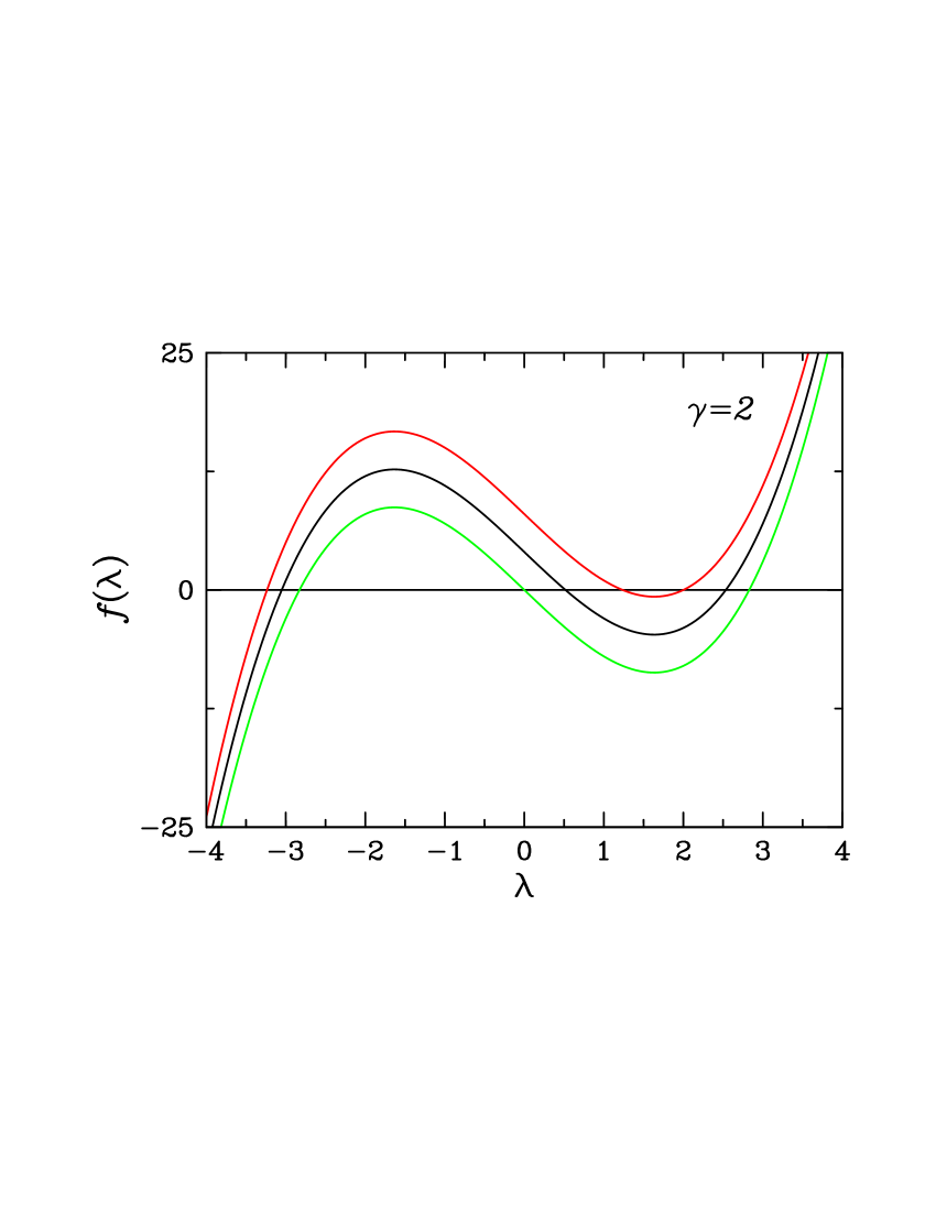
Figure 1: Plot of the cubic $f(\lambda)$ vs. $\lambda$. The curves from bottom to top correspond to $x_{A}-x_{B}=0$, 0.5 and 1.0. The interaction parameter is $\gamma=2$.

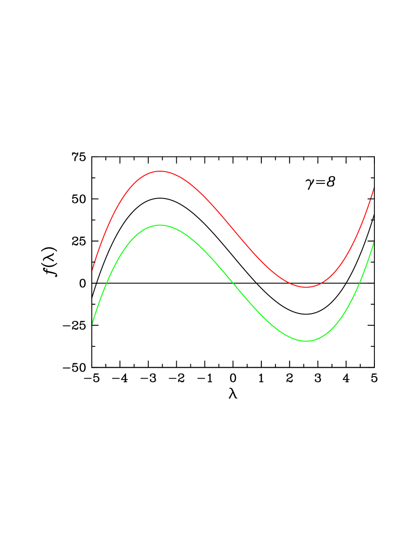
Figure 2: As for Fig. 1 but for an interaction parameter of $\gamma=8$.

In Fig. 1, $f(\lambda)$ is plotted for $(x_{A}-x_{B})=0$, 0.5 and 1 and for $\gamma=2$; Fig.2 is a similar plot for $\gamma=8$. For $(x_{A}-x_{B})=0$, $f(\lambda)=\lambda(\lambda^{2}-4-2\gamma)$, which has the roots $\lambda=0$ and $\lambda=\pm\sqrt{4+2\gamma}$. For $(x_{A}-x_{B})=1$, $f(\lambda)=(\lambda-2)[\lambda(\lambda+2)-2\gamma]$, which has the roots $\lambda=2$ and $\lambda=-1\pm\sqrt{1+2\gamma}$. The latter two values are the Lagrange multipliers in the single-species limit as obtained from the minimization of Eq. (IV) for $x_{B}=0$. Since the term $4\gamma(x_{A}-x_{B})$ in $f(\lambda)$ simply shifts the curves in Figs. 1 and 2 vertically, it is clear that there are always three real roots for the physical range of $(x_{A}-x_{B})$ values. For any positive value of $\gamma$, one root is always less than $-2$, a second lies in the range $0\leq\lambda\leq 2$ (more precisely in the range $0\leq\lambda\leq 2(x_{A}-x_{B})$) and a third in the range $\lambda\geq 2$. Substituting the coefficients given in Eq. (110) into Eq. (108) we find

$$|c_{0}|^{2}=\frac{\varepsilon(\lambda^{2}-4)^{2}}{4[x_{A}(\lambda+1)(\lambda-2)^{2}+x_{B}(\lambda-1)(\lambda+2)^{2}]}.$$ (112)

It is clear from this expression that the $\lambda<-2$ root makes $|c_{0}|^{2}$ negative. This root is therefore physically inadmissible and only the positive $\lambda$ roots are relevant. Eq. (112) together with Eq. (110) can be used in Eq. (107) to evaluate the energy. One finds the remarkably simple result

$$\bar{E}_{0}(l)-\frac{\gamma}{2}=x_{A}-\varepsilon+\lambda\varepsilon=x_{A}+(l-x_{A})(1-\lambda).$$ (113)

We now see that the smaller of the two positive $\lambda$ roots gives the lowest possible energy. This thus identifies the root in the range $0<\lambda<2$ as the one that is physically relevant Smyrnakis09 . For $\lambda$ in this range we observe that the ratios in Eq. (110) are negative, indicating that the phases in Eq. (106) were chosen incorrectly. The proper phases are $\chi_{1}=\pi$, $\chi_{2}=0$ and $\chi_{3}=\pi$.

The criterion for the existence of persistent currents at $l=x_{A}$ used in Ref. Smyrnakis09 is that the slope of $\bar{E}_{0}(l)$ in Eq. (113) at $l=x_{A}^{-}$ is negative, i.e., $\lambda>1$. The critical condition is thus $\lambda=1$, which from Eq. (111) gives the critical interaction strength Smyrnakis09

$$\gamma_{cr}=\frac{3}{4(x_{A}-x_{B})-2}=\frac{3}{2(4x_{A}-3)}.$$ (114)

In the $x_{A}=1$ limit this reduces to $\gamma_{cr}=3/2$ which is the value obtained at $l=1$ for the single-species system. To obtain the critical coupling at $l=x_{A}+n-1$, where $n=1$, 2,.., we write $\bar{E}_{0}(l)=l^{2}+\bar{e}_{0}(l)$ and use the fact that $\bar{e}_{0}(l)$ is periodic. The slope at $l=(x_{A}+n-1)^{-}$ is thus found to be

$$\left.\frac{d\bar{E}_{0}(l)}{dl}\right|_{l=(x_{A}+n-1)^{-}}=2n-1-\lambda.$$ (115)

If the root in the range $0<\lambda<2(x_{A}-x_{B})$ is used, the slope cannot be zero for any $n>1$. This is the basis of the claim made in Ref. Smyrnakis09 that persistent currents are not possible for $l>1$; seemingly, an arbitrarily small amount of the minority component $B$ has a profound effect on the possibility of persistent currents. For the single-species case, the energy is given by Eq. (113) with $x_{A}=1$, but the appropriate value of $\lambda$ is $\lambda=-1+\sqrt{1+2\gamma}$, which is not bounded as a function of $\gamma$. Using this value in Eq. (115), one finds that persistent currents are possible for all $n$ in this case, with a critical interaction strength of $\gamma_{cr,n}={(2n+1)(2n-1)}/{2}$. This is the result found earlier (Eq. (74)) using the Landau criterion. This comparison indicates an inconsistency. On the one hand, Eq. (115) does allow for persistent currents for $l>1$ in the single-species limit if the appropriate value of $\lambda$ is used. However, the two-species analysis requires that the root in the range $0<\lambda<2$ be used, which precludes the possibility of persistent currents for $l>1$ for any nonzero value of $x_{B}$. Since the energy functional in Eq. (IV) reduces to the single-species case when $x_{B}=0$, it would appear that taking the $x_{B}\to 0$ limit of the two-species analysis is problematic.

In order to explain this discrepancy it is useful to examine the behaviour of the coefficients in Eqs. (110) and (112) in the $x_{A}\to 1$ limit in more detail. These coefficients are determined by the root $\lambda$ that lies in the range $0\leq\lambda<2$. If $\gamma<4$, the limiting value of this root for $x_{A}\to 1$ is $\lambda=-1+\sqrt{1+2\gamma}$. This is the $\lambda$ value for the single-species case. Thus for this range of $\gamma$, one recovers the single-species values for all the coefficients. However, for $\gamma>4$, the root in the range $0\leq\lambda<2$ has the limiting value of 2 which is less than the $\lambda=-1+\sqrt{1+2\gamma}$ root. The limiting values of the coefficients do not correspond to the single-species values in this case.

The distinction between $\gamma<4$ and $\gamma>4$ is revealed more clearly by plotting the coefficients in these two cases as a function of $x_{B}$. We observe that the angular momenta carried by each of the species is given by

$$l_{A}=x_{A}\left(|c_{1}|^{2}+2|c_{2}|^{2}\right)=x_{A}+x_{A}\left(|c_{2}|^{2}-|c_{0}|^{2}\right)$$ (116)

and

$$l_{B}=x_{B}\left(-|d_{-1}|^{2}+|d_{1}|^{2}\right).$$ (117)

The change in angular momentum as $l$ is reduced from $x_{A}$ is associated with the transfer of weight from one angular momentum component to another. For example, for the $A$ species, the transfer takes place from the $m=1$ state to the $m=0$ or $m=2$ states, with respectively, a decrease or increase in angular momentum. For the $B$ species, the transfer takes place from the $m=0$ state to the $m=-1$ and $m=1$ states. Of interest is the relative magnitude of the angular momentum change $\Delta l_{s,m}$ that is associated with each angular momentum component. We therefore define the ratios $\Delta l_{s,m}/(-\varepsilon)$ where for example, $\Delta l_{A,0}/(-\varepsilon)=(-x_{A}|c_{0}|^{2})/(-\varepsilon)$. These ratios represent the fraction of the angular momentum change $-\varepsilon=l-x_{A}$ attributable to each of the angular momentum components.

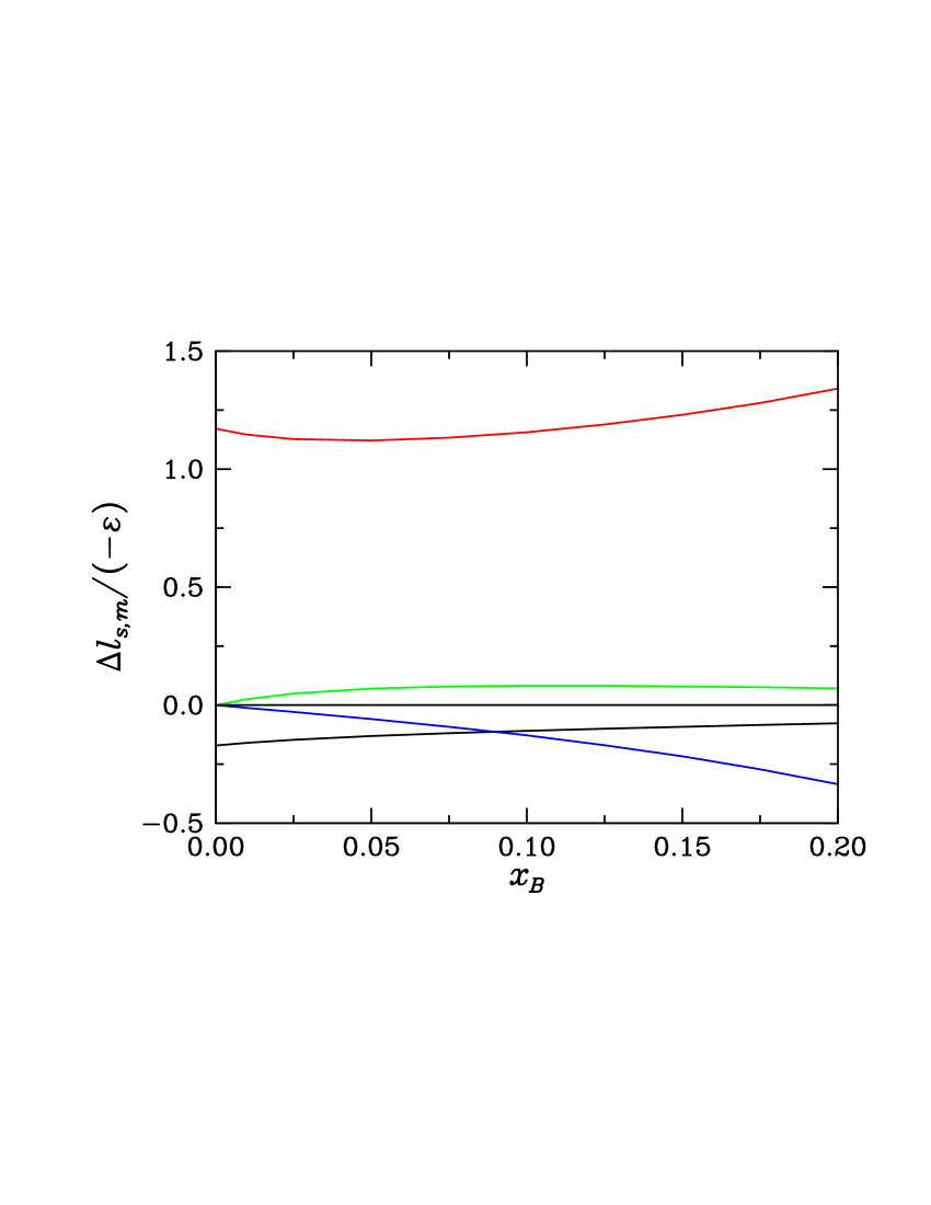
Figure 3: The angular momentum change carried by each of the wave function components relative to the total angular momentum change of $-\varepsilon$ as a function of $x_{B}$: red ($\Delta l_{A,0}$), black ($\Delta l_{A,2}$), green ($\Delta l_{B,-1}$), blue ($\Delta l_{B,1}$). The interaction parameter is $\gamma=2$.

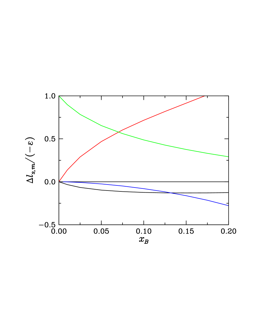
Figure 4: As in Fig. 3 but for $\gamma=8$.

In Fig. 3 we plot these ratios as a function of $x_{B}$ for $\gamma=2$; Fig. 4 gives similar plots for $\gamma=8$. For $\gamma=2$, we see that species $B$ carries a relatively small contribution of the angular momentum change. This contribution vanishes in the $x_{B}\rightarrow 0$ limit and the situation reverts to that of the single species which, as discussed above, is generally the case for $\gamma<4$. The situation for $\gamma>4$, however, is quite different. Fig. 4 for $\gamma=8$ shows that the angular momentum change is carried entirely by the $m=-1$ component of the $B$ species in the $x_{B}\rightarrow 0$ limit. The reason for this surprising result is that the relevant $\lambda$ root approaches 2 for $x_{B}\rightarrow 0$ when $\gamma>4$. Eq. (112) then gives $|c_{0}|^{2}\simeq(2-\lambda)^{2}\varepsilon/(4x_{B})$ and from Eq. (110) we find $|d_{-1}|^{2}\simeq\varepsilon/x_{B}$ for $x_{B}\rightarrow 0$, i.e. $l_{B}=-\varepsilon$ in this limit. The divergence of $|d_{-1}|^{2}$ as $x_{B}\rightarrow 0$ is indicating that the result can only be valid for a decreasingly smaller range of $\varepsilon$ since the normalization $1=|d_{-1}|^{2}+|d_{0}|^{2}+|d_{1}|^{2}$ must be preserved. In other words, the energy $\bar{E}_{0}(l)$, as given by Eq. (113), is meaningful in an interval of $l$ of decreasing size as $x_{B}\to 0$.

The above results call into question any conclusion regarding the possibility of persistent currents at higher angular momenta when $x_{A}$ approaches 1. In this limit, a more global perspective regarding the behaviour of the energy as a function of $l$ in the interval $x_{B}\leq l\leq x_{A}$ is required. We now give a general argument for the possibility of persistent currents at $l>1$ based on the assumption of continuity of the GP energy as a function of $x_{B}$. To exhibit this dependence we write $\bar{E}_{0}(l,x_{B})$ and consider this function in the limit of small $x_{B}$. In particular, we have $\bar{E}_{0}(n,x_{B})=\bar{E}_{0}^{A}(n)+\delta_{1}(x_{B})$ and $\bar{E}_{0}(n-\Delta l,x_{B})=\bar{E}_{0}^{A}(n-\Delta l)+\delta_{2}(x_{B})$ where $\bar{E}_{0}^{A}(l)=\bar{E}_{0}(l,x_{B}=0)$ is the energy of the single-species system. The assumption of continuity implies that $\delta_{1}(x_{B})$ and $\delta_{2}(x_{B})$ approach 0 as $x_{B}\to 0$. We then have $\bar{E}_{0}(n-\Delta l,x_{B})-\bar{E}_{0}(n,x_{B})=\bar{E}_{0}^{A}(n-\Delta l)-\bar{E}_{0}^{A}(n)+\delta_{2}(x_{B})-\delta_{1}(x_{B})$. By choosing $\gamma>\gamma_{{\rm cr},n}$, $\bar{E}_{0}^{A}(n-\Delta l)-\bar{E}_{0}^{A}(n)$ will have some fixed positive value. Thus, we can say that $\bar{E}_{0}(n-\Delta l,x_{B})-\bar{E}_{0}(n,x_{B})>0$ for $x_{B}$ sufficiently small. Since $\partial\bar{E}_{0}(l,x_{B})/\partial l|_{l=n^{-}}<0$, we conclude that $\bar{E}_{0}(l,x_{B})$ must have a local minimum between $l=n-\Delta l$ and $l=n$. This argument can be used for any $n$ and shows that persistent currents must be stable in the vicinity of $l=n$ if $x_{B}$ is sufficiently small and $\gamma$ is sufficiently large.

Although it is difficult to evaluate $\bar{E}_{0}(l,x_{B})$ for arbitrary $l$, the above general argument can be illustrated quantitatively by evaluating the energy at $l=1/2$. To do so, it is sufficient to assume four-component wave functions of the form

$$\psi_{A}=c_{-1}\phi_{-1}+c_{0}\phi_{0}+c_{1}\phi_{1}+c_{2}\phi_{2}$$ (118)

$$\psi_{B}=d_{-1}\phi_{-1}+d_{0}\phi_{0}+d_{1}\phi_{1}+d_{2}\phi_{2}.$$ (119)

Substituting these wave functions into Eq. (IV), we have

$$\bar{E}_{0}(l=1/2)=x_{A}\left(|c_{-1}|^{2}+|c_{1}|^{2}+4|c_{2}|^{2}\right)+x_{B}\left(|d_{-1}|^{2}+|d_{1}|^{2}+4|d_{2}|^{2}\right)$$

$$+\hskip 2.84526ptx_{A}^{2}\pi\gamma\int_{0}^{2\pi}d\theta|c_{-1}\phi_{-1}+c_{0}\phi_{0}+c_{1}\phi_{1}+c_{2}\phi_{2}|^{4}+x_{B}^{2}\pi\gamma\int_{0}^{2\pi}d\theta|d_{-1}\phi_{-1}+d_{0}\phi_{0}+d_{1}\phi_{1}+d_{2}\phi_{2}|^{4}$$

$$+\hskip 2.84526pt2x_{A}x_{B}\pi\gamma\int_{0}^{2\pi}d\theta|c_{-1}\phi_{-1}+c_{0}\phi_{0}+c_{1}\phi_{1}+c_{2}\phi_{2}|^{2}|d_{-1}\phi_{-1}+d_{0}\phi_{0}+d_{1}\phi_{1}+d_{2}\phi_{2}|^{2}.$$ (120)

The periodicity and reflection properties imply $c_{0}\left(\frac{1}{2}\right)=c_{1}^{*}\left(\frac{1}{2}\right)$ and $c_{-1}\left(\frac{1}{2}\right)=c_{2}^{*}\left(\frac{1}{2}\right)$, with analogous relations for the $d_{m}$ amplitudes. These relations reduce the number of variational parameters by half. We have in particular

$$|c_{0}|=|c_{1}|\equiv x, \quad|c_{-1}|=|c_{2}|\equiv y$$

$$\alpha_{1}=-\alpha_{0}, \quad\alpha_{-1}=-\alpha_{2}$$

$$|d_{0}|=|d_{1}|\equiv u, \quad|d_{-1}|=|d_{2}|\equiv v$$

$$\chi_{1}=-\chi_{0}, \quad\chi_{-1}=-\chi_{2}.$$ (121)

Using these definitions, the normalization constraints reduce to

$$x^{2}+y^{2}=\frac{1}{2},\quad u^{2}+v^{2}=\frac{1}{2}.$$ (122)

Furthermore, the angular momentum of each species is given by

$$l_{A}=x_{A}(-|c_{-1}|^{2}+|c_{1}|^{2}+2|c_{2}|^{2})=x_{A}(x^{2}+y^{2})$$ (123)

$$l_{B}=x_{B}(-|d_{-1}|^{2}+|d_{1}|^{2}+2|d_{2}|^{2})=x_{B}(u^{2}+v^{2}).$$ (124)

We thus see that normalization ensures that the total angular momentum has the required value of 1/2.

Using these results, the expression for the energy becomes

$$\bar{E}_{0}(1/2)=\frac{1}{2}+\frac{1}{2}\gamma+4x_{A}y^{2}+4x_{B}v^{2}$$

$$\hskip 6.54413pt+\hskip 2.84526ptx_{A}^{2}\gamma\Big{[}x^{4}+y^{4}+8x^{2}y^{2}+4x^{3}y\cos\beta\Big{]}+x_{B}^{2}\gamma\Big{[}u^{4}+v^{4}+8u^{2}v^{2}+4u^{3}v\cos\xi\Big{]}$$

$$\hskip 6.54413pt+\hskip 2.84526ptx_{A}x_{B}\gamma\Big{[}8xyuv\left\{\cos(\theta-\beta+\xi)+\cos(2\theta-\beta+\xi)\right\}+\hskip 2.84526pt4xyu^{2}\cos(\theta-\beta)+4x^{2}uv\cos(\theta+\xi)\Big{.}$$

. $$\hskip 71.13188pt+\hskip 2.84526pt2x^{2}u^{2}\cos\theta+2y^{2}v^{2}\cos(3\theta-2\beta+2\xi)\Big{]},$$ (125)

where we have defined the phase angles $\beta=3\alpha_{0}+\alpha_{2}$, $\xi=3\chi_{0}+\chi_{2}$ and $\theta=2(\alpha_{0}-\chi_{0})$. We see that the energy depends on these three independent phases and the two amplitudes $x$ and $u$. It clearly reduces to the single-species result in the $x_{B}\rightarrow 0$ limit.

For $x_{A}=1$, the energy is minimized for $\beta=\pi$ and a value of $x$ which is close to $1/\sqrt{2}$.. We do not expect this conclusion to change when $x_{A}$ is close to, but not exactly equal to 1. For these values of $x_{A}$, the term in Eq. (IV) proportional to $x_{B}^{2}$ is small and can be neglected. Setting $\beta=\pi$, the energy is approximately

$$\bar{E}_{0}(1/2)\simeq\frac{1}{2}+\frac{1}{2}\gamma+4x_{A}y^{2}+4x_{B}v^{2}+\hskip 2.84526ptx_{A}^{2}\gamma\Big{[}x^{4}+y^{4}+8x^{2}y^{2}-4x^{3}y\Big{]}$$

$$\hskip 6.54413pt+\hskip 2.84526ptx_{A}x_{B}\gamma\Big{[}-8xyuv\left\{\cos(\theta+\xi)+\cos(2\theta+\xi)\right\}-\hskip 2.84526pt4xyu^{2}\cos\theta+4x^{2}uv\cos(\theta+\xi)\Big{.}$$

. $$\hskip 71.13188pt+\hskip 2.84526pt2x^{2}u^{2}\cos\theta+2y^{2}v^{2}\cos(3\theta+2\xi)\Big{]},$$ (126)

From this we see that the phases $\theta$ and $\xi$ only appear in the last term proportional to $x_{B}$. It is clear that $\bar{E}_{0}$ is stationary with respect to these phases when they take the values 0 and $\pi$. To explore the various possibilities, we define the function

$$f(x,u,\xi,\theta)=-\hskip 2.84526pt8xyuv[\cos(\theta+\xi)+\cos(2\theta+\xi)]-4xyu^{2}\cos\theta$$

$$\hskip 1.42271pt+\hskip 2.84526pt4x^{2}uv\cos(\theta+\xi)+2x^{2}u^{2}\cos\theta+2y^{2}v^{2}\cos(3\theta+2\xi),$$ (127)

which is the quantity multiplying $x_{A}x_{B}\gamma$ in Eq. (126). This function is tabulated in Table 1 for various values of $\xi$ and $\theta$.

$\xi$	$\theta$	$f(x,u,\xi,\theta)$
0	0	$-16xyuv-4xyu^{2}+4x^{2}uv+2x^{2}u^{2}+2y^{2}v^{2}$
0	$\pi$	$4xyu^{2}-4x^{2}uy-2x^{2}u^{2}-2y^{2}v^{2}$
$\pi$	0	$+16xyuv-4xyu^{2}-4x^{2}uv+2x^{2}u^{2}+2y^{2}v^{2}$
$\pi$	$\pi$	$4xyu^{2}+4x^{2}uy-2x^{2}u^{2}-2y^{2}v^{2}$

Table 1: The function $f(x,u,\xi,\theta)$ defined in Eq. (IV) tabulated for various values of $\xi$ and $\theta$.

From this table it is clear that $\xi=0$, $\theta=\pi$ will give a lower energy than $\xi=\pi$, $\theta=\pi$. For $\xi=0$, $\theta=0$ we have

$$f(x,u,0,0)-f(x,-u,0,0)=8xuv(x-4y).$$ (128)

Since $x_{A}$ is close to 1, Eq. (126) is minimized for a value of $x$ close to $1/\sqrt{2}$ which is much larger than $y$. This implies that any minima of the function $f(x,u,0,0)$ will occur for negative values of $u$. But $u$ must be positive (recall $u=|d_{0}|$), so this case must be rejected. Finally, for $\xi=\pi$, $\theta=0$, we have

$$f(x,u,\pi,0)-f(x,-u,\pi,0)=-8xuv(x-4y).$$ (129)

The same argument implies that minima of $f(x,u,\pi,0)$ must occur at positive $u$. We are thus left with the two possibilities $\xi=0$, $\theta=\pi$ and $\xi=\pi$ and $\theta=0$. A comparison of the contour plots of $\bar{E}_{0}(x,u,\pi,0)$ and $\bar{E}_{0}(x,u,0,\pi)$ shows that the latter is the one that provides the lowest energy. For $x_{A}=0.95$ and $\gamma=2$, $\bar{E}_{0}(x,u,0,\pi)$ is minimized for $x_{min}\simeq 0.697$ and $u_{min}\simeq 0.677$. The value of $x_{min}$ found here is close to the value of 0.696 found for $x_{A}=1$. Not surprisingly, the $|c_{m}|^{2}$ coefficients are close to the values obtained in the single-species limit.

We will now use the value of $\bar{E}_{0}(1/2)$ to show that persistent currents are possible for $l>1$. To be specific, we consider $l=1+l^{\prime}$ with $0\leq l^{\prime}\leq 1$. Using the periodicity of $\bar{\epsilon}_{0}(l)$, we have

$${E}_{0}(1+l^{\prime})=1+2l^{\prime}+\bar{E}_{0}(l^{\prime}).$$ (130)

At $l=x_{A}$, Eq. (94) gives $\bar{E}_{0}(x_{A})=x_{A}+\gamma/2$. We then find that $\bar{E}_{0}(1+x_{A})-\gamma/2=1+3x_{A}=3.85$ for $x_{A}=0.95$. As explained earlier, this value is exact within the mean-field analysis. We next use Eq. (130) to obtain

$$\bar{E}_{0}\left(3/2\right)=2+\bar{E}_{0}\left(1/2\right).$$ (131)

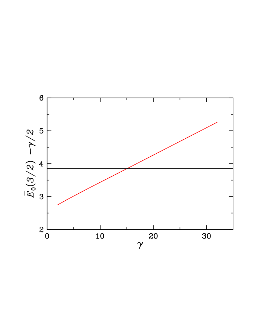
Figure 5: The energy at $l=3/2$ vs $\gamma$ for $x_{A}=0.95$. The horizontal line is the value of $\bar{E}_{0}(1+x_{A})-\gamma/2$.

In Fig. 5 we show the behaviour of $\bar{E}_{0}(3/2)-\gamma/2$ as a function of $\gamma$ for $x_{A}=0.95$. We see that $\bar{E}_{0}(3/2)$ becomes larger than $\bar{E}_{0}(1.95)$ at a value of $\gamma\simeq 15$. This implies the existence of a local minimum in the range $1.5<l<1.95$ and hence the possibility of persistent currents. The value $\gamma\simeq 15$ is clearly an upper bound to $\gamma_{cr}$ for this value of $x_{A}$.

The approximate behaviour of $\bar{E}_{0}(l)$ as a function of $l$ can be obtained by generating approximations to $\bar{e}_{0}(l)$. For $0\leq l\leq x_{B}$ and $x_{A}\leq l\leq 1$, $\bar{e}_{0}(l)-\gamma/2=l(1-l)$. From Eq. (113) we have $\bar{e}^{\prime}_{0}|_{l=x_{A}^{-}}=1-2x_{A}-\lambda$. The simplest approximation to $\bar{e}_{0}(l)$ in the range $x_{B}\leq l\leq x_{A}$ consistent with this information is

$$\bar{e}_{0}^{(1)}(l)-\gamma/2=l(1-l)+\lambda{(x_{A}-l)(l-x_{B})\over x_{A}-x_{B}}$$ (132)

An improved approximation is a fit that reproduces the value of $\bar{e}_{0}(l)$ at $l=1/2$. It takes the form

$$\bar{e}_{0}^{(2)}(l)-\gamma/2=l(1-l)+\lambda{(x_{A}-l)(l-x_{B})\over x_{A}-x_{B}}+\mu{(x_{A}-l)^{2}(l-x_{B})^{2}\over(x_{A}-x_{B})^{4}}$$ (133)

where $\mu=16[\bar{e}_{0}(1/2)-\gamma/2-1/4-\lambda(x_{A}-x_{B})/4]$. A third approximation ignores the information about the slope of $\bar{\epsilon}_{0}(l)$ at $l=x_{A}$ but includes the value at $l=1/2$. This approximation gives

$$\bar{e}_{0}^{(3)}(l)-\gamma/2=l(1-l)+\nu{(x_{A}-l)(l-x_{B})\over(x_{A}-x_{B})^{2}},$$ (134)

where $\nu=4(\bar{e}_{0}(1/2)-\gamma/2-1/4)$. These various approximations are plotted in Fig. 6 for $\gamma=16$. We expect the correct variation of $\bar{e}_{0}(l)$ to be bounded by the $\bar{e}_{0}^{(2)}(l)$ and $\bar{e}_{0}^{(3)}(l)$ curves; for $l\to 0.95$, $\bar{e}_{0}(l)$ should be closer to the $\bar{e}_{0}^{(2)}(l)$ curve but for $l\to 0.5$ it should be closer to the $\bar{e}_{0}^{(3)}(l)$ curve. We note that $\bar{e}_{0}^{(3)}(l)$ must give the correct behaviour in the $x_{A}\to 1$ limit.

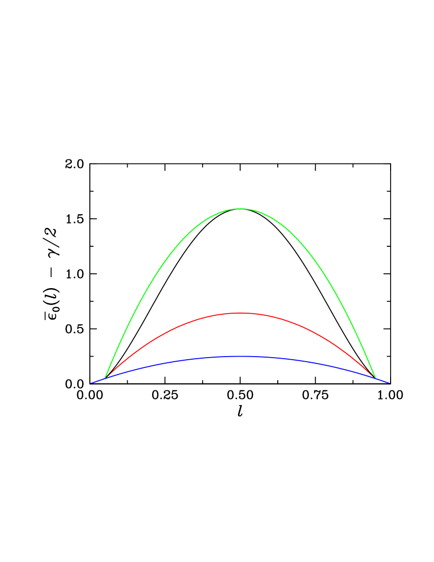
Figure 6: The function $\bar{e}_{0}(l)-\gamma/2$ plotted vs $l$ in different approximations. The blue curve is the function $l(1-l)$; the red, black and green curves are $\bar{e}_{0}^{(1)}$, $\bar{e}_{0}^{(2)}$ and $\bar{e}_{0}^{(3)}$ respectively. $\gamma=16$ and $x_{A}=0.95$.

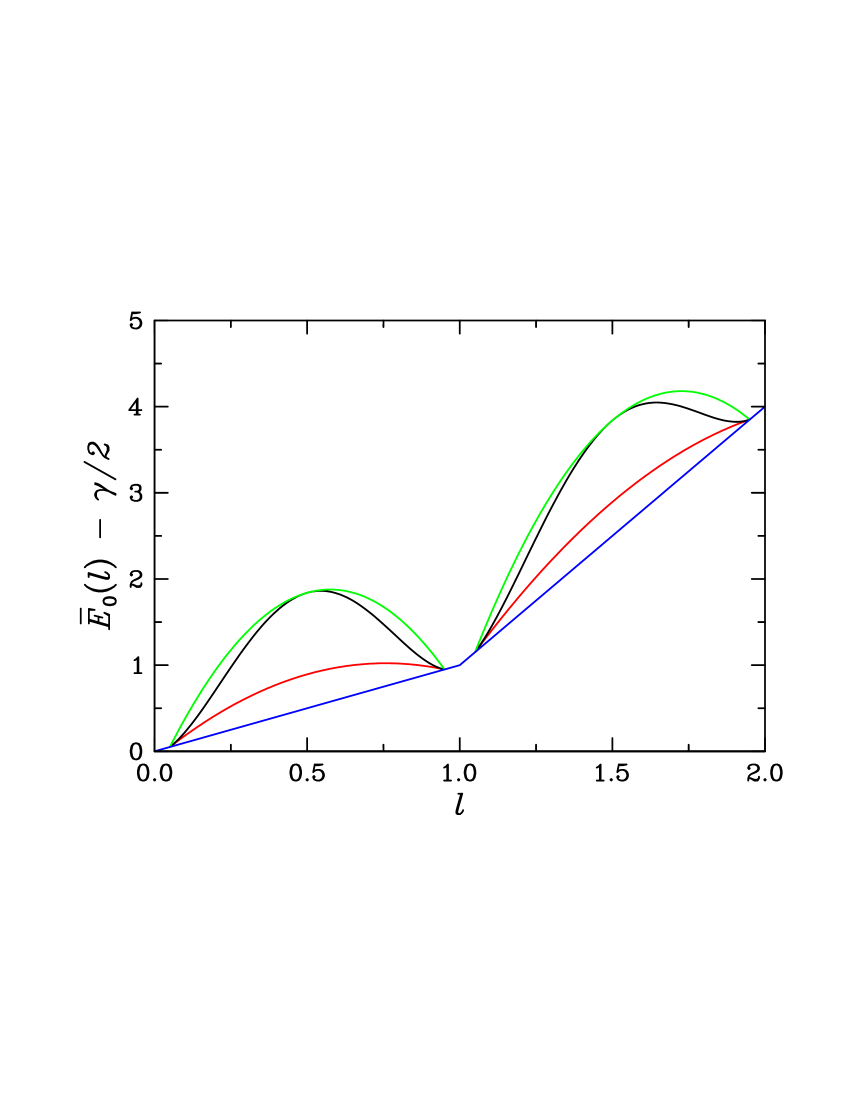
Figure 7: The energy $\bar{E}_{0}(l)-\gamma/2$ vs $l$ for $\gamma=16$ and $x_{A}=0.95$. The various curves correspond to the various approximations to $\bar{e}_{0}(l)$ shown in Fig. 6.

These different approximations can be used to determine corresponding approximations to $\bar{E}_{0}(l)$, which is plotted in Fig. 7 in the range $0\leq l\leq 2$ for $\gamma=16$. The red curve based on $\bar{e}_{0}^{(1)}(l)$ does not show a local minimum at $l=1.95$ as predicted by considerations of the slope of $\bar{E}_{0}(l)$ at this point. On the other hand, the black curve based on $\bar{e}_{0}^{(2)}(l)$ which includes the information about $\bar{e}_{0}(1/2)$ shows a local minimum below $l=1.95$ and demonstrates that persistent currents should be possible for $l$ between 1.5 and 2. Regarding persistent currents at $l=0.95$, the critical interaction strength according to Eq. (114) for $x_{A}=0.95$ is $\gamma_{\rm cr}\simeq 1.9$. For this value of $\gamma$, $\bar{e}_{0}^{(1)}(1/2)$ is actually quite close to to the true value $\bar{e}_{0}(1/2)$ as determined by the four-component wave function analysis. Thus the prediction of the critical interaction strength based on the slope of $\bar{E}_{0}(l)$ remains quite accurate in this case. However, it is clear that the slope of $\bar{E}_{0}(l)$ calculated at $l=(x_{A}+n-1)^{-}$, although correct, is not sufficient to provide a criterion for the existence of persistent currents for $n>1$. We have also extended the analysis to slightly smaller values of $x_{A}$ and arrive at similar conclusions. However, increasingly larger values of $\gamma$ are then required to achieve a local minimum between $l=1.5$ and $l=1+x_{A}$.

We finally mention the behaviour of $\bar{E}_{0}(l=1/2)$ when $x_{A}=1/2$. In this limit the expression for $\bar{E}_{0}(l)$ given in Eq. (94) is correct for all $l$ and gives in particular $\bar{E}_{0}(l=1/2,x_{A}=1/2)=1/2+\gamma/2$. This value is reproduced by Eq. (IV) at $x_{A}=1/2$ irrespective of the phases $\beta$ and $\xi$ since the minimum occurs for $\theta=\pi$ and $x=u=1/\sqrt{2}$, where all the $\beta$ and $\xi$ dependent terms have no effect since $y=v=0$. We note that the minimizing value of $\theta$ is the same as in the $x_{A}\to 1$ limit and anticipate that this will remain true for intermediate values of $x_{A}$ between $x_{A}=1/2$ and $x_{A}=1$. However, a more careful analysis of Eq. (IV) would be required to confirm this and to determine the remaining variational parameters that minimize the GP energy.

V Conclusions

In this paper we have extended to the two-species system Bloch’s original argument regarding the possibility of persistent currents in the idealized one-dimensional ring geometry. Strict periodicity of the energy $e_{\alpha}(L)$ defined in Eq. (1) is found to arise when the mass ratio $M_{A}/M_{B}$ is a rational number. By making a connection to the Landau criterion for the special case $M_{A}=M_{B}$, we show that persistent currents are in general possible at the discrete set of total angular momenta $L_{n}=nN\hbar$, except when the interaction parameters satisfy the condition in Eq. (76). The underlying reason for this limitation is the existence of excitations with a particle-like dispersion. This conclusion is consistent with the predictions of a mean-field analysis based on the GP energy functional. A detailed analysis of the GP energy in the vicinity of $l=x_{A}$, first carried out by Smyrnakis et al. Smyrnakis09 , indicates that persistent currents are possible at this angular momentum per particle if the interaction parameter exceeds the critical value given in Eq. (114). These authors go on to claim that persistent currents cannot arise for $l>1$ in the two-species system. However, a more detailed analysis of the global behaviour of the GP energy demonstrates that this conclusion is not valid. Quite generally, the properties of the two-species system evolve continuously to those of the single-species system as the concentration of the minority component is reduced. It would of course be of interest to verify these theoretical predictions experimentally. The recent experimental realization of toroidal Bose-Einstein condensates Ryu07 ; Ramanathan11 would suggest that experiments on two-species systems may soon be feasible.

References

(1) F. Bloch, Phys. Rev. A 7, 2187 (1973).
(2) J. Wilks, An Introduction to Liquid
Helium, (Clarendon Press, Oxford, 1970).
(3) E. M. Lifshitz andL. P. Pitaevskii, Statistical Physics, Part 2, (Butterworth-Heinemann, Oxford,
1980).
(4) J. Smyrnakis, S. Bargi, G. M. Kavoulakis, M.
Magiropoulos, K. Kärkkäinen, and S. M. Reimann,
Phys. Rev. Lett. 103, 100404 (2009).
(5) P. Tommasini, E. J. V. de Passos, A. F. R. de
Toledo Piza, M. S. Hussein and E. Timmermans, Phys. Rev. A 67,
023606 (2003).
(6) P. Ao and S. T. Chui, J. Phys. B 33, 535
(2000).
(7) C. J. Pethick and H. Smith, Bose-Einstein Condensation in Dilute Gases, 2nd ed. (Cambridge,
Cambridge, 2008).
(8) C. Ryu, M. F. Andersen, P. Cladé, Vasant Natarajan,
K. Helmerson, and W. D. Phillips, Phys. Rev. Lett 99 260401
(2007).
(9) A. Ramanathan, K. C. Wright, S. R. Muniz,
M. Zelan, W. T. Hill III, C. J. Lobb, K. Helmerson, W. D.
Phillips, and G. K. Campbell, Phys. Rev. Lett. 106, 130401
(2011).