Conductivity close to antiferromagnetic criticality

Abstract

We study the conductivity of a 3D disordered metal close to the antiferromagnetic instability within the framework of the spin-fermion model using the diagrammatic technique. We calculate the interaction correction $\delta\sigma(\omega,T)$ to the conductivity, assuming that the latter is dominated by the disorder scattering, and the interaction is weak. Although the fermionic scattering rate shows critical behaviour on the entire Fermi surface, the interaction correction is dominated by the processes near the hot spots, narrow regions of the Fermi-surface corresponding to the strongest spin-fermion scattering. Exactly at the critical point $\delta\sigma\propto[max(\omega,T)]^{3/2}$. At sufficiently large frequencies $\omega$ the conductivity is independent of the temperature, and $\delta\sigma\propto(\tau^{-1}-i\omega)^{-2}$, $\tau$ being the elastic scattering time. In a certain intermediate frequency range $\delta\sigma(\omega)\propto i\omega(\tau^{-1}-i\omega)^{-2}$.

Transport close to quantum criticality fascinates and challenges researchers in many fields of condensed matter, ranging from the physics of high-temperature superconductors and heavy-fermion materials to the conduction in graphene or granulated superconductors near the superconductor-insulator transitionSachdev (2011); v. Löhneysen et al. (2007). At low temperatures, the interplay of disorder and interactions inevitably plays an important role in transport. Efforts to investigate the conductivity near magnetic instabilities often rely on the spin-fermion modelAbanov et al. (2002): the conductivity is determined by low-energy fermionic excitations, interacting with collective bosonic spin modes that carry no charge yet become soft modes at the magnetic critical point.

If the interaction corrections to the conductivity are small, they can be analysed in the framework of the spin-fermion model using perturbation theory. For instance, for a 2D metal near a ferromagnetic (FM) instability the corrections can be found microscopicallyPaul et al. (2005) using the diagrammatic technique similar to the electron-electron interaction correctionsAltshuler and Aronov (1985); Zala et al. (2001) to the conductivity of a disordered metal.  A separate analysis is needed in the case of an antiferromagnetic (AFM) instability, characteristic of pnictide superconductors, certain heavy-fermion materials and possibly the cuprate systems and organic charge transfer salts. Near the AFM transition, the momenta of the lowest-energy spin fluctuations are large and close to the reciprocal vectors of the spin superlattice in the AFM phase. As a result, electrons strongly interact with spin fluctuations only close to narrow regions of the Fermi surface, the so-called “hot spots”, and can be scattered from one such region to another.

In a system without disorder the quasiparticle lifetime and weight vanish at the hot spots at low energies. The analysis of the Boltzmann transport equation concludedHlubina and Rice (1995), however, that the conductivity is dominated by weakly scattering “cold spots”. The role of impurities within the kinetic-equation approach was investigated by UedaUeda (1977) and RoschRosch (1999) who found a correction $\Delta\rho\propto T^{3/2}$ to the residual resistivity $\rho_{0}$ caused by impurities. The fractional power here was explained by the width of the “hot lines” $\propto T^{1/2}$ Rosch (1999). It is, however, unclear why such a quasiclassical Boltzmann approach should be applicable, considering, in particular, the singular scattering rate and vanishing quasiparticle weight. Another interesting question, which deserves a separate investigation, is related to the notion of impurity-induced ”local criticality”Si et al. (2001): the single-particle self-energy may become momentum independent $\Sigma\left(\mathbf{k,}i\omega\right)\simeq\Sigma\left(i\omega\right)$ and show singular behaviour on the entire Fermi surface away from the hot spot, that would manifest itself in the resistivity $\rho(T)$. As estimated in Ref. Wölfle and Abrahams (2011), such local scattering processes lead to the quasiparticle scattering time $\tau_{sp}^{-1}\left(T\right)\propto T^{3/2}$. This momentum-independent scattering rate implies a similar temperature dependence of $\Delta\rho$. The emergence of an impurities-induced local single-particle scattering rate is particularly interesting given the experimental indications in favour of local, i.e. momentum independent, criticality of electrons near the antiferromagnetic quantum critical pointsv. Löhneysen et al. (2007).

In this Letter we study microscopically transport in the spin-fermion model in the presence of impurities using the diagrammatic technique. We demonstrate that at sufficiently strong disorder and weak spin-fermion coupling the interaction corrections to the resistivity are dominated by processes near the hot spots. The quasiparticle self-energies in the “cold regions” also show critical behaviour, leading, however, to a smaller contribution to the resistivity correction. We find the conductivity dependency on temperature and frequency. In the zero-frequency low-temperature limit we recover the results previously known from the kinetic-equation approach.

Model. We consider for simplicity a spherical Fermi surface. A fermion can absorb or emit only a boson with momentum close to a certain large vector ${\bf Q}$ ($|{\bf Q}|\sim k_{F}$), determined by the geometry of the AFM spin superlattice in the AFM phase. In order to address the experimentally relevant case of an isotropic conduction we assume that there are three such (incommensurate) vectors, ${\bf Q}_{1}$, ${\bf Q}_{2}$, and ${\bf Q}_{3}$, of equal length and directed respectively along different coordinate axes. The fermions strongly interact with bosons only close to the “hot-spots”, points on the Fermi surface separated by the vectors ${\bf Q}_{n}$, Fig. 1. In our case the hot spots are three pairs of circles; an electron near each circle can be inelastically scattered to the corresponding circle in the opposite hemisphere.

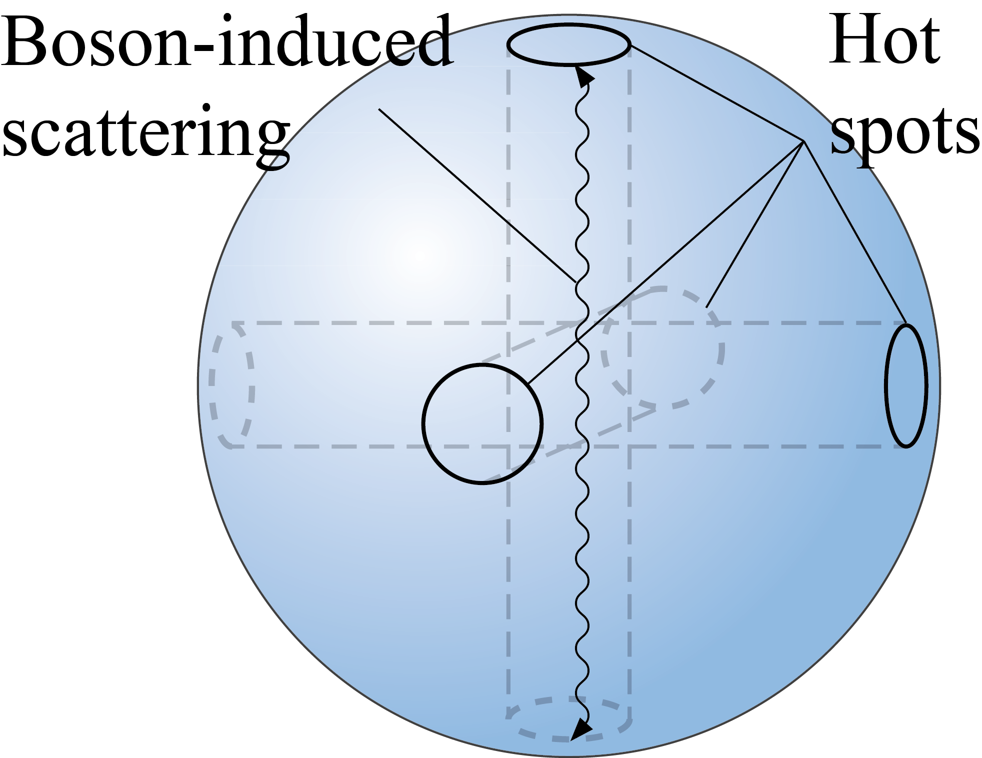
Figure 1: (Colour online) The Fermi surface.

The action of the spin-fermion model reads

$$S=\sum_{\sigma}\int_{x}{c}_{\sigma}^{\dagger}(x)\left[\partial_{\tau}+\xi\left(-i\nabla\right)+U(\mathbf{r})\right]{c}_{\sigma}(x)$$

$$-\frac{1}{2}\sum_{n}\int_{x,x^{\prime}}\mathbf{S}_{n}(x){D_{n}^{-1}(x-x^{\prime})}\mathbf{S}_{n}(x^{\prime})$$

$$+{g}\sum_{\sigma\sigma^{\prime}n}\int_{x}{c}_{\sigma}^{\dagger}\left(x\right)\mathbf{\boldsymbol{\sigma}}_{\sigma\sigma^{\prime}}{c}_{\sigma^{\prime}}\left(x\right)\mathbf{S}_{n}(x),$$ (1)

where ${c}_{\sigma}^{\dagger}\left(x\right)$ and ${c}_{\sigma}\left(x\right)$ are the Grassman fields for an electron (fermion) with spin $\sigma$, $x=\left(\mathbf{r,}\tau\right)$; $\mathbf{S}_{n}\left(x\right)$ is the bosonic field of the collective spin excitations; $n=1,2,3$ labels a pair of hot spot circles separated by the vector $\mathbf{Q}_{n}$, $g$ is the coupling constant between the bosons and the fermions, $\xi_{\mathbf{k}}\equiv\xi({\bf k})$ is the electron spectrum, ${D_{n}(x-x^{\prime})}$ is the propagator of the bosonic modes; the disorder is represented by the random potential $U(\mathbf{r})$, which acts on the fermions only. The fermion spectrum allows for the existence of the hot spots, i.e., points on the Fermi surface where $\xi_{{\bf k}+{\bf Q}}=\xi_{\bf k}$. We use the abbreviation $\int_{x}\cdots=\int d^{3}r\int_{0}^{\beta}d\tau\cdots$ and set $e=\hbar=1$. Also, below we suppress the bosonic index $n$, if the respective expression does not depend on it, and use conventions $k=\left(\mathbf{k},i\omega\right)$ and $\int_{k}\cdots=T\sum_{\omega}\int\frac{d{\bf k}}{(2\pi)^{3}}$.

The energies of all excitations in the spin-fermion model are limited by a phenomenological scale $\Lambda$, which separates the low energies involved in the transport phenomena from the high-energy modes responsible for the formation of the antiferromagnetism. The shape of the Fermi surface and the excitation spectra are assumed renormalised upon having integrated out all the higher-energy modes $\Lambda<\varepsilon\lesssim W$ Abanov et al. (2002), where $W\gg\Lambda$ is the microscopic bandwidth of the tight-binding Hamiltonian of the underlying lattice. The relative smallness of the cutoff $\Lambda$ allows one to linearise the fermionic spectrum $\xi_{\bf k}$ with respect to $\mathbf{k-k}_{\mathrm{F}}$.

We consider a system sufficiently close to the critical point, so that the collective spin excitations are the most important bosonic excitations in the model and one can disregard the other types of interaction. On the other hand, to address small interaction corrections to the conductivity of a disordered metal, observed in experiments, we assume that the dimensionless coupling constant, $\alpha\simeq{g^{2}}/{v_{F}}\ll 1$, is the very smallest parameter in the theory, which allows us to treat the interactions perturbatively. In principle, the renormalised bosonic propagator $D_{n}(i\Omega,\mathbf{q})$ depends on the coupling $g$. However, we assume below that the boson dynamics is characterised by the elastic scattering time $\tau$ of electrons and phenomenological energy scales independent of $g$.

The assumption of small $\alpha$ implies, in particular, that the conductivity is dominated by disorder scattering. For simplicity, the impurity scattering is assumed to be isotropic, and the disorder potential – weak and Gaussian; $\langle U(\mathbf{r})U(\mathbf{r}^{\prime})\rangle=(2\pi\rho_{F}\tau)^{-1}\delta({\bf r}-{\bf r}^{\prime})$, where $\rho_{F}=\frac{k_{F}^{2}}{2\pi^{2}v}$ is the density of states on the Fermi surface. The parameter $(\varepsilon_{F}\tau)^{-1}\ll 1$ is assumed to be the second smallest in the problem, $\varepsilon_{F}$ being the Fermi energy.

Perturbation theory. Under the assumptions that the bosonic modes are correlated on a short scale yet the spin-fermion coupling is weak, one can conveniently calculate the interaction corrections to the conductivity perturbatively. To the $0^{th}$ order in the interaction, the conductivity is given by the Drude contribution $\sigma_{0}\left(\omega\right)=({2}/{3})v^{2}\rho_{F}\left(\tau^{-1}-i\omega\right)^{-1}$, together with the weak-localisation and the electron-electron interaction corrections to it. Next we calculate the leading correction $\sigma_{2}\propto g^{2}$ in the spin-fermion coupling $g$.

Let us consider first the renormalisation of the fermion-boson interaction vertex by disorder. The first non-vanishing correction to the coupling $g$, Fig. 2, reads

$$\delta g({\bf q},i\omega,i\varepsilon)=\frac{g}{2\pi\rho_{F}\tau}\int\frac{d{\bf k}}{(2\pi)^{3}}G(\mathbf{k},i\varepsilon)G(\mathbf{k}+\mathbf{q},i\varepsilon+i\omega),$$ (2)

where $i\omega$ and $\mathbf{q}\simeq\mathbf{Q}$ are, respectively, the frequency and the momentum of the spin excitation at the vertex; $G(i\varepsilon,\mathbf{k})=\left[i\varepsilon-\xi_{\mathbf{k}}+i/(2\tau)\mathop{\rm sgn}\varepsilon\right]^{-1}$ is the disorder-averaged fermion propagatorAbrikosov et al. (1975). Because there are no excitations with energies larger than $\Lambda$, the integration is confined to narrow regions around the hot-spot circles, such that $|\xi_{\mathbf{k}},\xi_{{\bf k}+{\bf q}}|<\Lambda$. This allows one to integrate separately the two propagators near the two different hot-spot circles, arriving at a very small renormalisation of the coupling $\delta g/g\sim(\varepsilon_{F}\tau)^{-1}\mathop{\rm sgn}\left(\omega\right)\mathop{\rm sgn}\left(\omega+\varepsilon\right)$, which, as we show below, may be neglected when calculating the conductivity. Due to the large momentum transfer by the AFM bosonic fluctuations, $|{\bf q}|\sim|\mathbf{Q}|\sim k_{F}$, the renormalisation is fully perturbative, i.e. may be considered only to the leading order in the disorder potential, and does not involve the summation of the whole diffusion ladder, unlike the case of electron-electron or FM interactions, when the momentum scattering at the vertex is smallAltshuler and Aronov (1985); Zala et al. (2001).

Let us notice also that the Hartree contributions to the conductivity and to the quasiparticle scattering rates, that contain one boson propagator, (e.g., in Fig. 2b) vanish due to the symmetry of the spin-fermion interaction vertex. Indeed, such diagrams contain an independent summation of one interaction vertex with respect to the spin polarizations $\propto\sum_{\sigma}\boldsymbol{\sigma}_{\sigma\sigma^{\prime}}=0$.

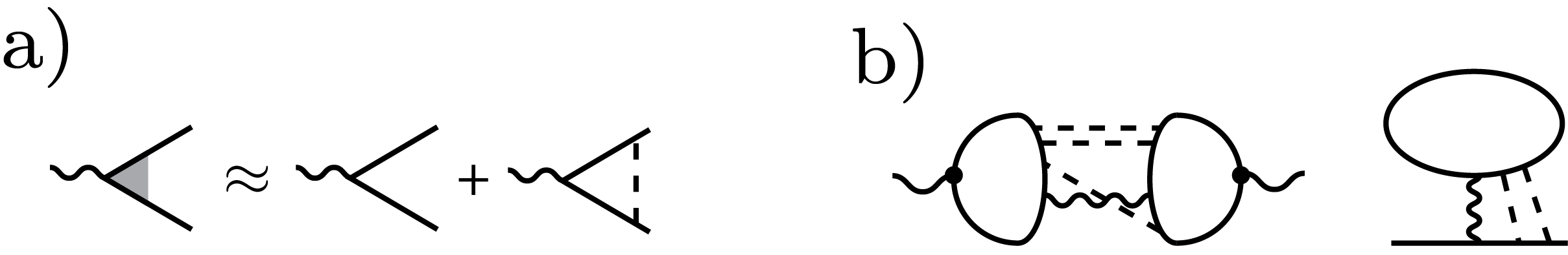
Figure 2: a)Renormalisation of the spin-fermion interaction vertex. b)Hartree contributions to the conductivity and to the fermion scattering rate.

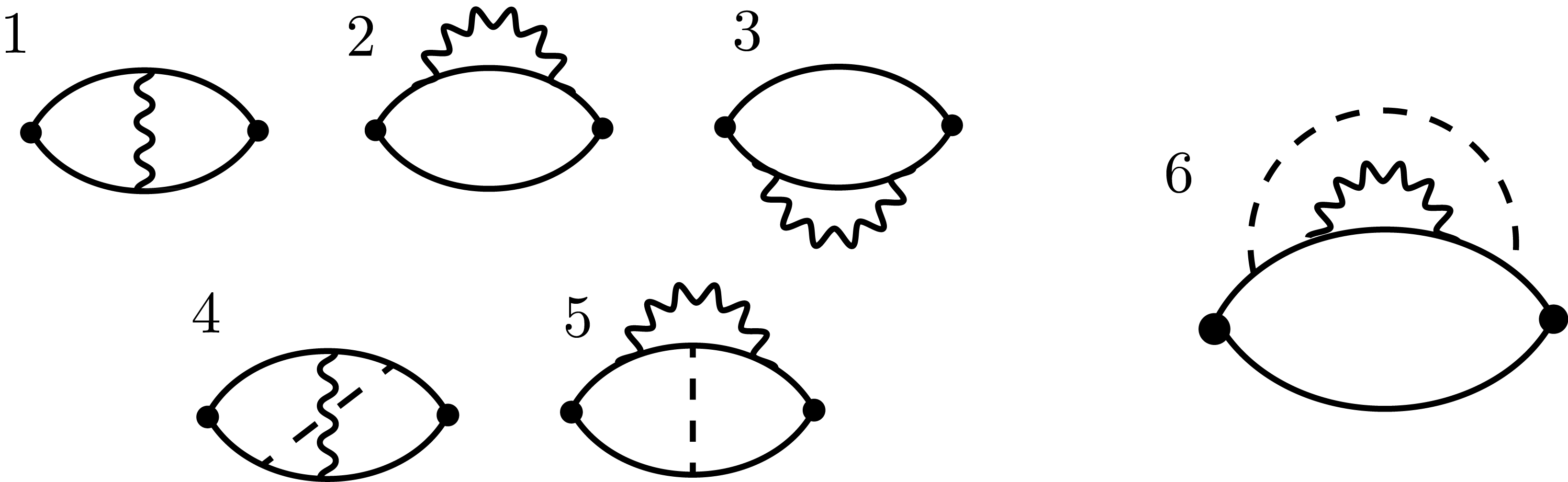
Figure 3: Interaction corrections to the conductivity. Diagrams 1-5 mimic processes close to the hot spots, while 6 is the contribution of electrons on the whole Fermi surface.

To the lowest order in interactions and in disorder strength the conductivity correction is given by diagrams 1-3 in Fig. 3 (thin solid lines correspond to the disorder-averaged electron propagators). Their contribution to the conductivity is given by the analytic continuation from the Matsubara to real frequencies, $i\omega\rightarrow\omega+i0$, of the quantity

$$\delta\sigma(i\omega)=\frac{\alpha v_{\parallel}k_{F}\int_{q}(\omega-|\Omega|)\theta\left(\omega-|\Omega|\right)D(i\Omega,{\bf q})}{\pi\omega{(\tau^{-1}+\omega)^{2}}},$$ (3)

where $q=\left(\mathbf{q},i\Omega\right)$ and $v_{\parallel}$ is the component of velocity at the hot spot parallel to the respective vector ${\bf Q}$. The analytic continuation reads

$$\delta\sigma(\omega)=-\frac{2i\alpha v_{\parallel}k_{F}\int D^{R}(\varepsilon,\mathbf{q})A(\omega,\varepsilon)\frac{d\varepsilon d^{3}q}{\left(2\pi\right)^{4}}}{\pi\omega{(\tau^{-1}-i\omega)^{2}}},$$ (4)

where $D^{R}(\varepsilon,\mathbf{q})$ is the retarded boson propagator, and $A\left(\omega,\varepsilon\right)=(\omega-\varepsilon)\left[n(\varepsilon)-n(\varepsilon-\omega)\right]$ with the Bose distribution function $n(\varepsilon)$.

Diagrams 4-6 in Fig. 3 contain one extra impurity line and represent the next-order corrections to the conductivity in the disorder strength, which are not accounted for by the renormalisation of the interaction vertex. We show in what immediately follows that, because of the large bosonic momenta, adding more impurity lines to diagrams 1-3 results in small corrections, that are perturbative in the disorder strength.

The straightforward evaluation of the diagram 4 shows that the corresponding contribution $\delta\sigma_{4}(i\omega)\sim\delta\sigma(i\omega)\mathcal{O}\left[(\varepsilon_{F}\tau)^{-1}\right]$ is suppressed by the small parameter $(\varepsilon_{F}\tau)^{-1}$ compared to diagrams 1-3, which can be understood as follows. The extra impurity line in diagram 4 adds to the respective integral one more momentum integration and two propagators, whose momenta are shifted by a large constant vector of the order of $k_{F}$ with respect to each other. This extra integration results in the relative smallness $(\varepsilon_{F}\tau)^{-1}$ of the diagram. A similar argument proves the smallness of the diagrams with crossing impurity lines in the usual disorder-averaging diagrammatic techniqueAbrikosov et al. (1975). Let us emphasise that this smallness is specific of the case to the large momentum scattering by the bosonic modes close to AFM criticality. If the electron dynamics is strongly affected by collective excitations with small momenta, e.g., FM fluctuationsPaul et al. (2005) or electron-electron interactionsAltshuler and Aronov (1985), then taking into account the whole diffusion ladder is necessary in place of the impurity lines for diagrams 4 and 5, as well as in the renormalisation of the spin-fermion interaction vertex.

Similarly, the contribution of diagram 5,

$$\delta\sigma_{5}(i\omega)\sim\alpha\tau^{-1}(\tau^{-1}+\omega)^{-2}\int_{q}D(i\Omega,\mathbf{q})$$ (5)

is also suppressed by the small parameter $(\varepsilon_{F}\tau)^{-1}$, compared to diagrams 1-3. However, Eq. (5) involves the summation of the boson propagator over all Matsubara frequencies, unlike Eq. (3), where the frequency summation is restricted to $|\Omega|<|\omega|$. This difference can make diagram 5 important at sufficiently low frequencies $\omega$. However, the temperature dependencies of both diagrams are determined by a few terms with $\Omega\sim T$ in the sums in Eqs. (5) and (3), and we can neglect the temperature dependency contribution of the diagram 5 so long as $\varepsilon_{F}\tau\gg 1$. $\delta\sigma_{5}(\omega=0,T=0)$ amounts to a contribution to the residual conductivity due to the spin fluctuations and may be disregarded in what follows. Similarly, one can neglect the diagrams for the conductivity that correspond to the renormalisation of the interaction vertex since $\varepsilon_{F}\tau\gg 1$.

Let us proceed to diagram 6 in Fig. 3. This interaction correction comes from electrons near the whole Fermi surface, unlike the previously considered diagrams 1-5, which correspond to processes near the hot spots. Indeed, anywhere on the Fermi surface an electron can be scattered into a hot spot, where its dynamics is impeded by spin fluctuations, cf. diagram 3 in Fig. 4. The value of the diagram 6 in Fig. 3

$$\delta\sigma_{6}(i\omega)\sim(\Lambda\tau)^{-1}\delta\sigma(i\omega)$$ (6)

is small compared to the value $\delta\sigma(i\omega)$ of diagrams 1-3 due to the small parameter $(\Lambda\tau)^{-1}\ll 1$, which can be understood as follows. On one hand, the extra smallness, $\sim(\varepsilon_{F}\tau)^{-1}$, comes from the extra impurity line. On the other hand, the diagram contains an extra largeness in it, $\sim\varepsilon_{F}/\Lambda$,– the ratio of the area of the Fermi surface to the characteristic size of the hot spots. The combination of the two factors leads to Eq. (6).

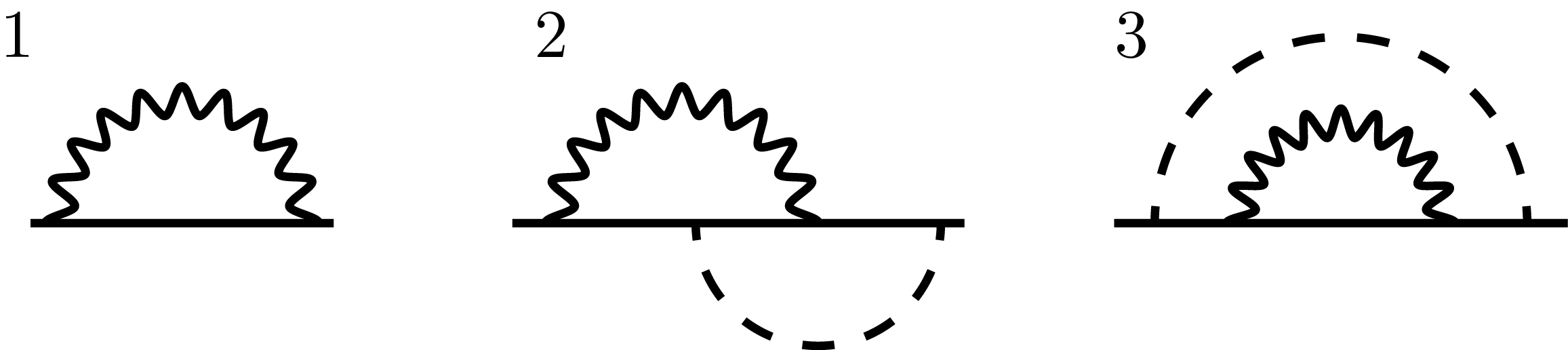
Figure 4: Interaction corrections to the scattering rate. Diagrams 1 and 2 describe scattering close to the hot spots, while 3 is an isotropic contribution to the scattering on the whole Fermi surface.

Thus, we have shown that to the leading order in disorder and interactions the conductivity is given by Eq. (3), corresponding to diagrams 1-3 in Fig. 3. To the first order in $\alpha$ the conductivity reads

$$\sigma\left(\omega\right)=\frac{2}{3}v^{2}\rho_{F}\left[{\tau^{-1}+\delta\tau^{-1}-i\omega\left(1+\lambda\right)}\right]^{-1},$$ (7)

where we introduced

$$\delta\tau^{-1}=-\frac{6\pi\alpha}{k_{F}\omega}\frac{v_{\parallel}}{v}\int{Im}D^{R}(\varepsilon,{\bf q})A(\omega,\varepsilon)\frac{d\varepsilon d{\bf q}}{(2\pi)^{4}},$$ (8)

$$\lambda=-\frac{6\pi\alpha}{k_{F}\omega^{2}}\frac{v_{\parallel}}{v}\int{Re}D^{R}(\varepsilon,{\bf q})A(\omega,\varepsilon)\frac{d\varepsilon d{\bf q}}{(2\pi)^{4}}.$$ (9)

The limit of low frequencies and temperatures. To make further progress at sufficiently small $\omega$ and $T$ we consider the most general form of the overdamped boson propagator that follows from the effective Ginzburg-Landau-type description:

$$D^{R}_{n}(\varepsilon,{\bf q})=-\sum_{\pm}\left[{\xi^{-2}+({\bf q}\pm{\bf Q})^{2}-i\varepsilon k_{F}^{2}\gamma^{-1}}\right]^{-1}$$ (10)

at $|\varepsilon|\ll\varepsilon_{F}^{2}\gamma^{-1}$. For $|\varepsilon|\gg\varepsilon_{F}^{2}\gamma^{-1}$, $D_{n}^{R}\propto\varepsilon^{-2}$. The scale $\gamma$ characterises elastic and inelastic scattering of the bosons. If the latter is attributable to electron-hole pairs, $\gamma=4\pi vv_{\parallel}k_{F}g^{-2}$. However, being a parameter of the boson propagator, $\gamma$ should be regarded as an independent phenomenological scale in the spin-fermion model and may come, e.g., from disorder scattering.

Substituting Eq. (10) into Eq. (8) yields $\delta\tau^{-1}=\frac{3\alpha\zeta(3/2)}{4\sqrt{2\pi}}\frac{v_{\parallel}}{v}\frac{T^{3/2}}{\gamma^{1/2}}$ for $(k_{F}\xi)^{2}\gg\gamma T^{-1}$ and $\omega=0$. While at $(k_{F}\xi)^{2}\ll\gamma T^{-1}$ and $\omega=0$ it holds that $\delta\tau^{-1}=\frac{\pi\alpha}{2}\frac{v_{\parallel}}{v}\frac{T^{2}k_{F}\xi}{\gamma}$. Similarly, for $T=0$ and finite frequencies $\delta\tau^{-1}=\frac{\alpha\sqrt{2}}{5\pi}\frac{v_{\parallel}}{v}\frac{\omega^{3/2}}{\gamma^{1/2}}$. The crossover between these regimes is described by the expression

$$\delta\tau^{-1}=\alpha\frac{v_{\parallel}}{v}\frac{T^{\frac{3}{2}}}{\gamma^{\frac{1}{2}}}\Phi\left(\frac{\gamma}{(k_{F}\xi)^{2}T},\frac{\omega}{T}\right)$$ (11)

with the scaling function

$$\Phi(y,z)=\frac{3}{2\pi^{2}z}\int\frac{x(z-x)t^{2}\left(\frac{1}{e^{x}-1}-\frac{1}{e^{x-z}-1}\right)}{(y+t^{2})^{2}+x^{2}}dxdt.$$ (12)

In particular, in the dc limit the correction to the resistivity due to the spin fluctuations at the AFM critical point reads

$$\delta\rho=\alpha C\frac{v_{\parallel}T^{\frac{3}{2}}}{v^{2}k_{F}^{2}\tau^{2}\gamma^{\frac{1}{2}}},$$ (13)

where $C=\frac{9\pi^{\frac{3}{2}}\zeta(3/2)}{4\sqrt{2}}=23.14..$, which up to a numerical coefficient matches the result obtained within the kinetic-equation approachUeda (1977); Rosch (1999).

High frequencies. At larger $\omega$ the frequency dependency of the conductivity can be found regardless of the particular form of the boson propagator. If the frequency is very large, the cutoff $\Lambda$ of the excitation energies in the spin-fermion model should be chosen larger than $\omega$ to ensure the existence of quasiparticles that can absorb a quantum $\omega$.

Let us assume first that the bosonic dynamics is determined by certain energy scales independent of the cutoff $\Lambda$. Then one can neglect the bosonic frequencies $\Omega$ in comparison with the large $\omega$ in Eq. (3). Making the analytic continuation and introducing the average value of the spin fluctuations $\langle S^{2}\rangle=-\int_{q}D(i\Omega,{\bf q})$, we arrive at

$$\delta\sigma(\omega)=-\frac{\alpha v_{\parallel}k_{F}}{\pi(\tau^{-1}-i\omega)^{2}}\langle S^{2}\rangle.$$ (14)

The result (14) has a simple physical interpretation. At very high frequencies the spin fluctuations may be considered frozen and equivalent to static disorder. The appropriate modification of the elastic scattering time, averaged with respect to angles, estimates $\delta\langle 1/\tau\rangle\sim\alpha\langle S^{2}\rangle/k_{F}$ and causes a correction $\delta\sigma\sim(\delta\tau^{-1})\partial\sigma_{0}/\partial\tau^{-1}$ to the Drude conductivity $\sigma_{0}$. As is necessary, this correction matches Eq. (14).

Intermediate frequencies. Let us proceed to the intermediate frequencies; $\omega$ exceeds the temperature $T$, but is smaller than the smallest characteristic energy of the boson dynamics, e.g., the bosonic scattering rate $\varepsilon_{F}^{2}\gamma^{-1}$.

Then at $|\Omega|<\omega$ the integral $\int D(i\Omega,{\bf q})\frac{d{\bf q}}{(2\pi)^{3}}$ is nearly independent of $\Omega$, because the value of $\Omega$ affects the boson propagator only on a sufficiently small momentum interval, while the rest of the integral is accumulated on a greater interval.

Thus, in Eq. (3) we may set $\int D(i\Omega,{\bf q})(d{\bf q})\approx\int D(0,{\bf q})(d{\bf q})$. Then the frequency summation in Eq. (3) and the analytic continuation to real frequencies yield

$$\delta\sigma(\omega)\propto-i\omega(\tau^{-1}-i\omega)^{-2},$$ (15)

independently of the form of the bosonic propagator.

Discussion. Spin-fermion interactions modify the quasiparticle self-energy part on the whole Fermi surface. Away from the hot spots the modification

$$\Sigma_{lc}(i\varepsilon)\sim-i\alpha(k_{F}\Lambda\tau)^{-1}\int_{q}\theta(|\varepsilon|-|\Omega|)D(i\Omega,{\bf q})\mathop{\rm sgn}\varepsilon.$$ (16)

is given by diagram 3 in Fig. 4. It is momentum-independent and “locally critical”, corresponding to the scattering rate $\tau_{lc}^{-1}\propto const+T^{3/2}$. Let us notice that Eqs. (8), (9), and (16) hold for an arbitrary boson propagator and can be used to analyse transport in, e.g., a system with a two-dimensional spin dynamicsv. Löhneysen et al. (2007). In arbitrary dimensions $d$, it holds that $\tau_{lc}^{-1}\propto const+T^{d/2}$.

We demonstrated, however, that the interaction correction to the conductivity near the AFM instability is dominated by the processes near the hot spots, corresponding to diagrams 1-3 in Fig. 3. We have found the dependency of the conductivity on frequency $\omega$ and temperature $T$. In the limit $\omega=0$ we recover the temperature dependencies of the interaction correction to the conductivity previously known from the kinetic equation analysis; $\delta\sigma\propto T^{3/2}$ and $\delta\sigma\propto T^{2}$ at the critical point and away from it respectively. At $T=0$ we find $\delta\sigma\propto\omega^{3/2}$. At sufficiently high frequencies the correction is independent of temperature and a particular form of the spin propagator. At very high and moderate frequencies the dependency is given by Eqs. (14) and (15), respectively.

Acknowledgements. We appreciate useful discussions with B.N. Narozhny and P. Wölfle.

References

- Sachdev (2011) S. Sachdev, Quantum Phase Transitions (Cambridge University Press, 2011).
- v. Löhneysen et al. (2007) H. v. Löhneysen, A. Rosch, M. Vojta, and P. Wölfle, Rev. Mod. Phys. 79, 1015 (2007).
- Abanov et al. (2002) A. Abanov, A. V. Chubukov, and J. Schmalian, Adv. Phys. 52, 119 (2002).
- Paul et al. (2005) I. Paul, C. Pepin, B. N. Narozhny, and D. L. Maslov, Phys. Rev. Lett. 95, 017206 (2005).
- Altshuler and Aronov (1985) B. L. Altshuler and A. G. Aronov, in Electron-electron interactions in disordered systems, edited by A. L. Efros and M. Pollak (North-Holland, Amsterdam, 1985).
- Zala et al. (2001) G. Zala, B. Narozhny, and I. Aleiner, Phys. Rev. B 64, 214204 (2001).
- Hlubina and Rice (1995) R. Hlubina and T. M. Rice, Phys. Rev. B 51, 9253 (1995).
- Ueda (1977) K. Ueda, J. Phys. Soc. Japan 43, 1497 (1977).
- Rosch (1999) A. Rosch, Phys. Rev. Lett. 82, 4280 (1999).
- Si et al. (2001) Q. Si, S. Rabello, K. Ingersent, and J. L. Smith, Nature 413, 804 (2001).
- Wölfle and Abrahams (2011) P. Wölfle and E. Abrahams, Phys. Rev. B 84, 041101(R) (2011).
- Abrikosov et al. (1975) A. A. Abrikosov, L. P. Gorkov, and I. E. Dzyaloshinski, Methods of Quantum Field Theory in Statistical Physics (Dover, New York, 1975).