Non-local order parameters for the 1D Hubbard model

Abstract

We characterize the Mott insulator and Luther-Emery phases of the 1D Hubbard model through correlators that measure the parity of spin and charge strings along the chain. These non-local quantities order in the corresponding gapped phases and vanish at the critical point $U_{c}=0$. The Mott insulator consists of bound doublon-holon pairs, which in the Luther-Emery phase turn into electron pairs with opposite spins, both unbinding at $U_{c}$. The behavior of the parity correlators can be captured by an effective free spinless fermion model.

The Hubbard model and its extensions have been widely used to investigate the behavior of strongly correlated electrons in several condensed matter systems ranging from Mott insulators (MI) to high-$T_{c}$ superconducting materials. Recently, the progress in ultracold gas experiments that use fermionic atoms trapped into optical lattices has opened the way to the direct simulation of the Hubbard model and the observation of the predicted MI phase MOTT . Since the Mott transition is of Berezinskii Kosterlitz Thouless (BKT) type, the MI phase does not admit a local order parameter; instead the transition point corresponds to the vanishing of some topological order, possibly described by appropriate nonlocal quantities RESO ; NAVO . A progress in this direction has been achieved in the related field of the bosonic Hubbard models, where MI and Haldane insulator phases have been characterized by means of non-local string parameters, inspired by the correspondence of the bosonic system with spin-1 Hamiltonians at low energy near integer filling DBA ; GIAMARCHI . One of these parameters is related to the parity correlator $O_{P}(r)=\langle e^{2i\pi\sum_{j=i}^{i+r}S_{z,i}}\rangle$, with $S_{z,i}=\frac{1}{2}(n_{i}-\nu)$ measuring the parity of the deviation of the occupation number $n_{i}$ with respect to the filling $\nu$ in a string starting from the site $i$, ending to the site $i+r$. The non-vanishing value of the parity parameter $O_{P}=\lim_{r\to\infty}O_{P}(r)$ in the insulating phase has been observed with in situ imaging in experiments on ultracold bosonic ⁸⁷Rb atoms ENDRES .

In this Letter we address the study of nonlocal string-type correlators to inspect the gapped phases of the fermionic Hubbard model. The expected role of antiferromagnetic (AF) correlations has so far driven the attention mainly to the study of Haldane type string correlators; these were found to vanish algebraically, together with $O_{P}(r)$ in the Luttinger liquid regime KCNZ . On the other hand, in the large Coulomb repulsion limit the Hubbard Hamiltonian at half-filling is known to reduce to the AF Heisenberg Hamiltonian, for which the parity string correlator reduces trivially to the identity, the wavefunction being frozen to the sector with only one electron per site. Since in the MI phase the number of doubly occupied sites (doublons) and empty sites (holons) is non-vanishing at any finite value of the interaction (as also observed experimentally MOTT ), it is reasonable to expect that an appropriate parity parameter could characterize the crossover from the Heisenberg to the Luttinger liquid limit, marking the existence of the MI phase.

The local 4-dimensional vector space on which an electron Hamiltonian acts is typically generated by applying to the vacuum operators forming a $su(4)$ algebra, with three Cartan generators. Consequently, we can introduce two independent parity correlators $O_{P}^{(\nu)}$, defined as:

$$O_{P}^{(\nu)}(r)=\left\langle e^{2i\pi\sum_{j=i}^{i+r}S_{z,i}^{(\nu)}(r)}\right\rangle,$$ (1)

with index $\nu=c,s$, namely the “charge” and “spin” generalizations of the parity correlator $O_{P}(r)$. Here $S_{z,i}^{(\nu)}$ are the spin and pseudospin operators defined respectively as $S_{z,i}^{(s)}=\frac{1}{2}(n_{i,\uparrow}-n_{i,\downarrow})$ and $S_{z,i}^{(c)}=\frac{1}{2}(n_{i}-1)$, with $n_{i\sigma}=c_{i\sigma}^{\dagger}c_{i\sigma}$, $\sigma=\uparrow,\downarrow$, $c_{i\sigma}^{\dagger}$ creating a fermion at site $i$ with spin $\sigma$. By means of bosonization and DMRG analysis, we will show that each $O_{P}^{(\nu)}$ orders in the corresponding gapped phase: MI for $\nu=c$, with open charge gap, and Luther Emery (LE) for $\nu=s$, with open spin gap. The $O_{P}^{(\nu)}$ vanish with the gap at the BKT transition point where the correlation length becomes infinite.

The Hubbard model is described by the Hamiltonian

$$\mathcal{H}= -\sum_{\langle ij\rangle\sigma}(c_{i\sigma}^{\dagger}c_{j\sigma}+c_{j\sigma}^{\dagger}c_{i\sigma})+U\sum_{i}n_{i\uparrow}n_{i\downarrow}$$ (2)

where the overlap integral $U$ gives the on-site contribution of Coulomb repulsion, and energy is expressed in units of the tunneling amplitude.

The bosonized form of the half-filled Hubbard Hamiltonian at low-energy is known to give rise to two continuum models describing separately the spin and charge sectors Giamarchibook . The latter is described by the Hamiltonian

$$H_{c}= \int dx\left\{\frac{v_{c}}{2\pi}\left[K_{c}\pi\Pi_{c}^{2}+\frac{1}{K_{c}}(\partial_{x}\Phi_{c})^{2}\right]\right.$$

$$-\left.\frac{2U}{(2\pi\alpha)^{2}}\cos(\sqrt{8}\Phi_{c})\right\}$$ (3)

with

$$v_{c}=v_{F}\left(1+\frac{U}{\pi v_{F}}\right)^{1/2}\quad K_{c}=\left(1+\frac{U}{\pi v_{F}}\right)^{-1/2}.$$ (4)

Here $\Phi_{c}$ is the compactified boson describing the charge excitations with velocity $v_{c}$, and $\Pi_{c}=\partial_{x}\Theta_{c}/\pi$ is its conjugate momentum ($\alpha$ is a cutoff). At the BKT transition point $U=0$, we have $K_{c}=1$. The bosonic field in the spin sector $\Phi_{s}$ is governed by equations which can be obtained from (3) and (4) by replacing $U\to-U$ and $c\to s$. The spin-charge transformation $c_{j\downarrow}\to(-1)^{j}c_{j\downarrow}^{\dagger}$, that implies $S_{z,j}^{(c)}\to S_{z,j}^{(s)}$, in the present bosonization analysis corresponds simply to the change $\Phi_{c}\leftrightarrow\Phi_{s}$. In fact, we have used the continuum prescriptions used in Ref. Giamarchibook where $S^{z}(x)=\frac{\partial_{x}\Phi_{s}(x)}{\sqrt{2}\pi}$ and $J^{z}(x)=\frac{\partial_{x}\Phi_{c}(x)}{\sqrt{2}\pi}$.

For $U>0$, we get $K_{s}>1$: the cosine term in $H_{s}$ is (marginally) irrelevant and the spin excitations are gapless and governed by an ordinary Gaussian model. Meanwhile, $K_{c}<1$ and a charge gap is generated by the relevant cosine term in $H_{c}$. As a consequence, the field $\Phi_{c}$ is pinned in one of the classical minima of the cosine term, i.e. $\Phi_{c}=\frac{2\pi m}{\sqrt{8}}$, $m\in\mathbb{Z}$, while $\Phi_{s}$ does not order. For $U<0$, just the same occurs with inverted roles $\Phi_{c}\leftrightarrow\Phi_{s}$. In the continuum limit one can realize that the parity operators become GIAMARCHI ; Nakamura03

$$O_{P}^{(\nu)}(r) \approx\langle\cos[\sqrt{2}\Phi_{\nu}(r)]\cos[\sqrt{2}\Phi_{\nu}(0)]\rangle.$$

Hence in the MI phase at $U>0$, $O_{P}^{(c)}$ turns out to be non vanishing. In the $U<0$ case instead the LE phase is characterized by nonzero $O_{P}^{(s)}$. The two Haldane type string correlators $O_{S}^{(\nu)}(r)=\langle S_{z,i}^{\nu}e^{2i\pi\sum_{j=i}^{i+r}S_{z,i}^{(\nu)}(r)}S_{z,i+r}^{(\nu)}\rangle$ give instead $O_{S}^{(\nu)}(r)\approx\langle\sin[\sqrt{2}\Phi_{\nu}(r)]\sin[\sqrt{2}\Phi_{\nu}(0)]\rangle$ where the same argument suggests that these are both asymptotically vanishing in the two gapped phases. From the above derivation, we can conjecture that a necessary and sufficient condition for having an asymptotically non vanishing charge (spin) parity correlator in the Hubbard model is the opening of a gap in the charge (spin) sector, so that $O_{P}^{(\nu)}$ do configure as order parameters for the gapped phases of the Hubbard model.

Below we support our previous argument providing a quantitative estimation of the parity string parameter in the MI phase. This is achieved by means of numerical analysis using the density matrix renormalization group (DMRG) algorithm on finite size chains with periodic boundary conditions (PBC’s). The analysis requires very precise and reliable data; in fact, the computing effort is significant due to both the slowdown caused by PBC’s and the high sensitivity of the correlations contained in $O_{P}^{(\nu)}(r)$ with respect to numerical errors. Hence we have chosen to consider chain sizes from $L=10$ to $L=50$ and $1024$ DMRG states. The curves of $O_{P}^{(c)}(r)$ plotted in Fig.1 for $L=50$ evidence clearly a fast convergence to the asymptotic values for high interactions as well as a progressive increase of the parity order with $U$.

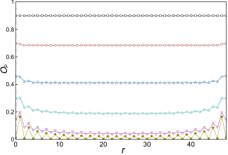
Figure 1: Parity correlator $O_{P}(r)$ for a periodic chain with $L=50$ as a function of the string length $r$. The sequences of data refer to $U=0.1,$1.0, 2.0, 3.0, 5.0, 10.0 (in ascending order).

The presence of two sequences for even and odd $r$ that tend toward the same asymptotic limit also signals that the spin parity correlator $O_{P}^{(s)}(r)=(-1)^{r}O_{P}^{(c)}(r)$ has a uniform part $[O_{P}^{(s)}(2r+1)+O_{P}^{(s)}(2r)]/2$ that goes smoothly to zero for $U>0$. The opposite mechanism holds for negative values of the interaction.

Exactly at $U=0$ both parity orders are absent and $O_{P}^{(c)}(r)=O_{P}^{(s)}(r)$ as required by the spin-charge symmetry. Here, an analytic calculation of $O_{P}^{(\nu)}(r)$ can be performed independently for both spin species by using the Wick theorem and evaluating Toeplitz determinants. An estimation of the asymptotic behavior gives $O_{P}^{(c)}(r)\sim r^{-1}$ at $U=0$ Abanov11 .

We have explicitly evaluated the order parameter $O_{P}^{(c)}$ in the MI phase and plotted it in Fig.2 for several values of $U$. The asymptotic values have been extrapolated from the finite-size scaling of the quantity $O_{P}^{(c)}(L/2)$ in a periodic chain of length $L$. For the fits, we have made use of functions $O_{P}(r)=O_{P}+Ar^{-\gamma}e^{-r/\xi}$ obtaining a good convergence. Interestingly, as evidenced in the inset of Fig.2, for small $U$ we get $\gamma=1$ and $A>0$, and for strong interactions we obtain $\gamma=1/2$ and $A<0$; while for intermediate values the best fit seems to be a combination of the two functions.

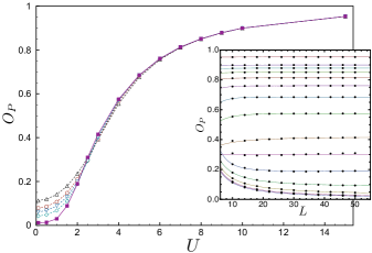
Figure 2: The charge parity order parameter measured at half chain $O_{P}^{(c)}(L/2)$ as a function of the local interaction $U$. We have considered PBC’s and finite chain lengths from $L=10$ to $L=50$ in step of 4, a sequence for which the ground state of the Hubbard model is unique. We have plotted the curves for $L=10$ (up triangles), $L=14$ (circles), $L=18$ (down triangles), $L=26$ (rhombs). The filled squares represent the finite size scaling values to $L=\infty$ obtained by the fits shown in the inset.

The non vanishing of $O_{P}^{(c)}$ implies the existence of bound doublon-holon pairs; their correlation length increases by decreasing $U$ becoming infinite at the transition, when pairs finally unbind. The quasi long-range AF order of the MI phase suggests that such pairs are diluted in an AF background of single electrons. The spin-charge transformation that maps positive $U$ Hamiltonian at half-filling into negative $U$ case at zero magnetization allows to extend the same type of analysis to the LE phase, which is then characterized at any filling by bound pairs of single electrons with opposite spin.

Based on the above scenario, we construct an approximation scheme that aims at isolating the relevant degrees of freedom (charges) to describe the actual role of $O_{P}^{(\nu)}$ in the Hubbard model. Since the operator $e^{i\pi n_{j}}=(-1)^{n_{j}}$ changes sign whenever the site $j$ is singly occupied, no matter its spin orientation, we choose to represent the original electronic creation operators $c_{i\sigma}^{\dagger}$ in terms of a spinless fermion $f_{i}^{\dagger}$ and Pauli operators $\sigma_{i}^{a}$, $a=x,y,z$ acting on a spin part. The mapping, schematized in Table 1,

spinful fermion	$|0\rangle$	$|\uparrow\rangle$	$|\downarrow\rangle$	$|\uparrow\downarrow\rangle$
spinless fermion $\otimes$ $\sigma$-spin	$|0\rangle$$|+\rangle$	$|1\rangle$$|+\rangle$	$|1\rangle$$|-\rangle$	$|0\rangle$$|-\rangle$

Table 1: Mapping from electrons to spinless fermions and $\sigma$-spins.

is identified by the unitary transformation

$$c_{i\uparrow}^{\dagger} =c_{i\uparrow}^{\dagger}(1-n_{i\downarrow})+c_{i\uparrow}^{\dagger}n_{i\downarrow}=f_{i}^{\dagger}P_{i}^{+}+(-1)^{i}f_{i}P_{i}^{-}$$

$$c_{i\downarrow}^{\dagger} =c_{i\downarrow}^{\dagger}(1-n_{i\uparrow})+c_{i\downarrow}^{\dagger}n_{i\uparrow}=(f_{i}^{\dagger}-(-1)^{i}f_{i})\sigma_{i}^{-}$$

with $P_{i}^{\pm}=\frac{1\pm\sigma_{i}^{z}}{2}$. Interestingly, the interaction term for the $c$-fermions simply becomes a chemical potential shift for $f$-fermions, namely $U\sum_{i}n_{i\uparrow}n_{i\downarrow}=U(N-\sum_{i}n_{i}^{f})/2$, where $N=\sum_{i,\sigma}n_{i\sigma}$. According to this picture, the spin and pseudospin operators are $\mathbf{S}_{j}^{(s)}=f_{j}^{\dagger}f_{j}\boldsymbol{\sigma}_{j}$ and $\mathbf{S}_{j}^{(c)}=f_{j}f_{j}^{\dagger}\boldsymbol{\sigma}_{j}$; conversely, we have $\boldsymbol{\sigma}_{j}=\mathbf{S}_{j}+\mathbf{J}_{j}$.

After the mapping the model in Eq.(2) becomes

$$\mathcal{H}= -\sum_{ij}\left[f_{i}^{\dagger}f_{j}Q_{ij}-2(-1)^{i}f_{i}^{\dagger}f_{j}^{\dagger}R_{ij}+\mathrm{H.c.}\right]$$

$$+\frac{U}{2}\left(N-\sum_{i}f_{i}^{\dagger}f_{i}\right),$$ (5)

where $Q_{ij}=(\boldsymbol{\sigma}_{i}\cdot\boldsymbol{\sigma}_{j}+1)/2$ is just the swap operator in the $\sigma$-spin state and $P_{ij}^{(S)}=(1-\boldsymbol{\sigma}_{i}\cdot\boldsymbol{\sigma}_{j})/4$ is the projector onto the singlet. Notice that (5) is invariant under global $\sigma$-spin rotations.

The form (5) for the Hubbard model holds in arbitrary dimension, and its terms are quadratic with respect to $f$-fermions. Since $O_{P}^{(\nu)}$ can be entirely expressed in terms of $f_{i}$, a possible strategy consists on tracing out the $\sigma$-spins by some mean-field approximation. In fact, exploiting the symmetries of the Hubbard model one can easily realize that $\langle Q_{ij}\rangle=1/2$ is an exact identity on the states on which the hopping term in (5) is non-vanishing. Moreover, we set the parameter $\alpha\equiv\langle R_{ij}\rangle$ in a phenomenological way by equating the ground state (GS) energy obtained from the spinless quadratic model with the exact energy coming from the Bethe-Ansatz solution LIWU . Within this approximation Eq.(5) is diagonalized in Fourier space, obtaining

$$H=\sum_{k\in BZ}\Lambda_{k}\left[\eta_{k}^{\dagger}\eta_{k}-\frac{1}{2}\right]+\frac{U(2N-L)}{4}\>,$$

with spectrum $\Lambda_{k}=-\cos k+\sqrt{16\alpha^{2}\cos^{2}k+U^{2}/4}$ and $\eta_{k}$ are the new fermionic modes. In the thermodynamical limit (TL), the energy density $e_{GS}$ at half-filling $\nu=1$ is given by $e_{GS}=\frac{U}{4}-\frac{1}{2\pi}\int_{-\pi/2}^{\pi/2}\mathrm{d}k\>\sqrt{16\alpha^{2}\cos^{2}k+U^{2}/4}.$ It is interesting to observe that the model is gapless only for $U=0$, where for $\alpha=1$ $e_{GS}$ assumes the exact value of the non-interacting case. For $U>0$ the number of singly occupied states $\nu_{f}$ is increasing and the pair-singlet states start to interact.

We are interested in calculating the parity operator $O_{P}^{(c)}(r)=\langle e^{i\pi\sum_{j=i}^{i+r}(n_{j}^{f}-1)}\rangle$, that can be rewritten as

$$O_{P}^{(c)}(r) =\left\langle\prod_{j=i}^{i+r}(2f_{j}^{\dagger}f_{j}-1)\right\rangle=\left\langle\prod_{j=i}^{i+r}A_{j}B_{j}\right\rangle$$

having defined $A_{j}=(f_{j}^{\dagger}+f_{j})$ and $B_{j}=(f_{j}-f_{j}^{\dagger})$. Making use of the Wick theorem, $O_{P}^{(c)}(r)$ can be expressed as a determinant LSM61

$$O_{P}^{(c)}(r)=\left|\begin{array}[]{ccccc}G_{0}&G_{1}&G_{2}&\cdots&G_{i,i+r}\\ -G_{1}&G_{0}&-G_{1}&\cdots\\ G_{2}&G_{1}&G_{0}&\cdots\\ \vdots&\vdots&\vdots&\ddots&\cdots\\ G_{i+r,i}&&&\vdots&G_{0}\end{array}\right|=\det(\mathbf{G}).$$ (6)

where $\mathbf{G}$ is a block Toeplitz matrix of dimension $(r+1)\times(r+1)$, whose entries are the one-body correlation functions $G_{r}=\langle(f_{j}^{\dagger}-f_{j})(f_{j+r}^{\dagger}+f_{j+r})\rangle$, whose expressions in the TL are

$$G_{r}=\begin{cases}\frac{U}{2\pi}\int_{0}^{\pi}\mathrm{d}k\>\frac{\cos(kr)}{\sqrt{16\alpha^{2}\cos^{2}(k)+U^{2}/4}},&r\;\mathrm{even}\\ (-1)^{j}\frac{4\alpha}{\pi}\int_{0}^{\pi}\mathrm{d}k\>\frac{\cos(kr)\cos(k)}{\sqrt{16\alpha^{2}\cos^{2}(k)+U^{2}/4}},&r\;\mathrm{odd}\end{cases}$$

with the property that $G_{0}=2\nu_{f}-1$, $G_{r}=2\mathrm{Re}(\langle f_{j}^{\dagger}f_{j+r}\rangle)$ for $r$ even and $G_{r}=2\mathrm{Re}(\langle f_{j}^{\dagger}f_{j+r}^{\dagger}\rangle)$ for $r$ odd. The blocks in (6) are of size $2\times 2$. We must distinguish the cases of $r$ even or odd, since they give rise to two different sequences. In particular, here we stick to the case $r$ odd, where the block matrix is of even dimension.

The analytical calculation of $O_{P}^{(c)}$ in the TL for some values of $U$ in the $f$-fermion approximation yields to the curve plotted in Fig.3, evidentiating the expected non vanishing of the charge parity order for $U>0$. The parameter $\alpha$ has been determined by requiring $e_{GS}(U,\alpha)=e_{ex}(U)$, where $e_{ex}$ is the exact result LIWU . Remarkably, such equality admits a solution for every $U$, which belongs to a narrow interval below $\alpha=1$, as shown in the inset of Fig.3. This means that in the pair-creation processes in (5) the $\sigma$-spin state is very close to the singlet. In the limit $U\gg 1$ the energy becomes $e_{GS}(\alpha)\approx-4\alpha^{2}/U$ that gives $\alpha(U\to\infty)=\sqrt{\log 2}\approx 0.83$, by comparison with the energy density of the Heisenberg model coming from the large-$U$ expansion of the Hubbard model at $\nu=1$. The result for $O_{P}^{(c)}$ is also quantitatively in accordance with the DMRG data in the large $U$ region, where our assumptions on the AF nature of short-ranged correlations noi10 are more justified.

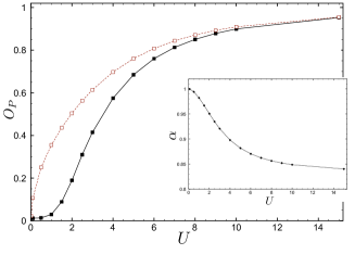
Figure 3: The parity order $O_{P}^{(c)}$ calculated according to Eq.(6) as a function of $U$ (dashed line) in the MI phase of the effective model (5) with $\alpha$ as in the inset figure, determined by tuning the spinless fermion energy to the exact Hubbard value. The results are compared with the numerical curve (continuous line) obtained for the Hubbard model and shown in Fig.2.

In conclusion, our work unveils that two (charge and spin) hidden parity string correlators play the role of order parameters for the gapped phases of the Hubbard model. In the bosonization approach these are found to be asymptotically finite only in the corresponding gapped MI and LE phases, and vanish with the gap at BKT transition point. The result is cleanly confirmed by DMRG numerical analysis. The emerging physical scenario is that of an insulator in which bound pairs of doublons and holons move in a AF background of single electrons. In the LE regime the role of doublons and holons and that of up and down electrons are exchanged. The picture allows to derive an effective free spinless fermion model which captures correctly the presence of non local order, and its vanishing at the transition. The spinless model is exact in the limit of large $U$ thus complementing the standard strong-coupling description with $t-J$ model.

The parity order is suitable for experimental detection by high resolution imaging ENDRES in ultracold Fermi gases. Possibly, some of the features described here could persist in two dimensions, where the localization of bound pairs could take place along one dimensional stripes. The scenario is quite suggestive also from the perspective of high-$T_{c}$ materials: the presence of bound doublon-hole pairs in the undoped insulator could play a role upon doping in the onset of the superconducting phase.

The present analysis could be further exploited to extended Hubbard models DOMO ; AAA , to describe other topologically ordered phases; noticeably, the fully gapped phase characterized by non vanishing charge and spin gaps should correspond to the non vanishing of both $O_{P}^{(\nu)}$’s. Work is in progress along these lines.

M.R. acknowledges support from the EU-ERC project no. 267915 (OPTINF) .

References

- (1) R. Jördens et al., Nature (London) 455, 204 (2008); U. Schneider et al., Science 322, 1520 (2008).
- (2) R. Resta, and S. Sorella, Phys. Rev. Lett. 82, 370 (1999)
- (3) M. Nakamura, and J. Voit, Phys. Rev. B 65 153110 (2002)
- (4) E.G. Dalla Torre, E. Berg, and E. Altman, Phys. Rev. Lett. 97, 260401 (2006).
- (5) E. Berg, E. G. Dalla Torre, T. Giamarchi, and E. Altman, Phys. Rev. B 77, 245119 (2008).
- (6) M. Endres et al., Science 334, 200 (2011).
- (7) H.V. Kruis, I.P. McCulloch, Z. Nussinov, and J. Zaanen, Phys. Rev. B 70, 075109 (2004).
- (8) T. Giamarchi, Quantum Physics in One Dimension, Oxford University Press, Oxford, 2004.
- (9) M. Nakamura, Physica B 329-333, 1000 (2003).
- (10) A.G. Abanov, D.A Ivanov, and Y. Qian, J. Phys. A: Math. Theor. 44, 485001 (2011).
- (11) E. H. Lieb, F.Y. Wu, Phys. Rev. Lett. 20, 1445 (1968).
- (12) E. Lieb, T. Schultz and D. Mattis, Ann. Phys. 16, 407 (1961).
- (13) M. Roncaglia, C. Degli Esposti Boschi, and A. Montorsi, Phys. Rev. B 82, 233105 (2010).
- (14) F. Dolcini, and A. Montorsi, Nucl. Phys. B 592, 563 (2001),
- (15) A. Aligia, et al., Phys. Rev. Lett. 99, 206401 (2007).