Turing patterns and apparent competition in predator-prey food webs on networks

Abstract

Reaction-diffusion systems may lead to the formation of steady state heterogeneous spatial patterns, known as Turing patterns. Their mathematical formulation is important for the study of pattern formation in general and play central roles in many fields of biology, such as ecology and morphogenesis. In the present study we focus on the role of Turing patterns in describing the abundance distribution of predator and prey species distributed in patches in a scale free network structure. We extend the original model proposed by Nakao and Mikhailov by considering food chains with several interacting pairs of preys and predators. We identify patterns of species distribution displaying high degrees of apparent competition driven by Turing instabilities. Our results provide further indication that differences in abundance distribution among patches may be, at least in part, due to self organized Turing patterns, and not necessarily to intrinsic environmental heterogeneity.

I Introduction

Reaction-diffusion systems, in which two or more species interact locally and diffuse through the medium, have long been focus of studies in many different fields, such as Physics, Chemistry and Biology. Part of the interest in these systems is related to their potential to form self-organized spatio-temporal patterns, like traveling and spiral waves murray_livro_v1 or stationary patterns, called Turing patterns murray_livro .

Working on the problem of morphogenesis turing Turing derived general analytical conditions for the formation of stationary patterns in reaction-diffusion systems under a mechanism today called diffusion driven instability (or Turing instability). Despite the specific nature of the original problem, the work led to a large number of applications in chemistry and biology, both theoretical murray_artigo1 ; murray_leopard ; murray_artigo2 ; meinhardt ; kishimoto ; baurmann and, more recently, empirical bansagi ; yamaguchi ; sawai . A key theoretical contribution was provided by Mimura and Murray murray_artigo2 , who applied Turing’s idea to understand patchiness in continuously distributed predator-prey populations.

Recently, Nakao and Mikhailov nakao proposed a discrete version of the prey-predator model of Mimura and Murray murray_artigo2 in which the species are organized in patches, instead of being continuously distributed in space. The patches are represented by nodes of a complex network such that predators and preys interact locally in each patch and diffusion occurs through connected nodes. The Turing patterns obtained in nakao present significant differences when compared to the ones obtained in the analogous system which considers space as a continuous medium.

In the present work, we extend of the model of Nakao and Mikhailov nakao by considering food chains with more than two species. We study the dynamics of several pairs of preys and predators that interact by consuming common preys. We show that the Turing patterns of population density displayed by the system present nontrivial correlations in the abundance distributions. In particular, we observe the emergence of strong competition between preys of adjacent species in the food chain, despite the fact that no direct competition between them are included in the equations. These correlations are strictly related to diffusion and correspond to a new mechanism of apparent competition, driven by Turing instabilities instead of local interactions. We characterize these patterns using numerical simulations and mean field approximations. We also discuss the relevance of these results to patterns of species distribution in real trophic systems.

II Dynamical model

In order to consider more complex reaction diffusion systems we extend the model introduced by Nakao and Mikhailov nakao to food chains composed by several species of preys and predators. We assume that each prey species has a primary predator associated to it, forming a pair. The pairs in the food chain are hierarchically coupled by secondary predation relations. Thus, the prey in the first pair is consumed by its main predator and also by the predator in the second pair, though with the lower intensity $\gamma$. Similarly, the prey of the second pair is consumed primarily by its associated predator and also by the predator of the third pair, and so on. Only the last species of prey in this ordered chain is consumed exclusively by its main predator as, illustrated by the diagram in figure 1.

The environment where these interactions take place consists of a network of patches. Species-species interactions, as described by the food chain, occur locally in each patch and the coupling between patches is exclusively due to diffusion, which is possible if the patches are connected in the network.

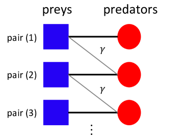
Figure 1: (Color online) Hierarchical food chain with three pairs of preys and predators. Each predator is linked to the previous prey (secondary predation) with strength $\gamma$.

The equations describing this dynamical system are given by:

$$\frac{d}{dt}u_{i}^{(l)}(t) =f(u_{i}^{(l)},v_{i}^{(l)})-\gamma u_{i}^{(l)}v_{i}^{(l+1)}+\epsilon\displaystyle\sum_{j}L_{ij}u_{j}^{(l)}$$

$$\frac{d}{dt}v_{i}^{(l)}(t) =g(u_{i}^{(l)},v_{i}^{(l)})+\phi\gamma u_{i}^{(l-1)}v_{i}^{(l)}+\sigma\epsilon\displaystyle\sum_{j}L_{ij}v_{j}^{(l)},$$ (1)

where $u_{i}^{(l)}(t)$ and $v_{i}^{(l)}(t)$ represent the populations of preys and predators at time $t$ respectively. The label $l=1,2,3,\cdots$ index the prey-predator pair.

The functions $f$ and $g$ describe the local interaction between preys and predators of each pair (also called reaction functions). The terms proportional to $\gamma$ represent the secondary predation relations between adjacent pairs and the parameter $\phi$ accounts for the ratio between predator gain and prey loss in the secondary interaction.

The parameters $\epsilon$ and $\sigma$ are, respectively, the prey mobility and the ratio between predator and prey mobilities. The matrix $L$ stands for the Laplacian matrix and accounts for the diffusion of populations across connected sites. For undirected networks $L$ is symmetric with $L_{ij}=A_{ij}-k_{i}\delta_{ij}$, where $A$ is the Adjacency Matrix and $k_{i}$ the degree of node $i$. The adjacency matrix defines the topology of the network and is given by $A_{ij}=1$ if nodes $i$ and $j$ are connected and $A_{ij}=0$ if they are not. The degree $k_{i}=\sum_{j}A_{ij}$ is the number of connections of node $i$.

The term $\sum_{j}L_{ij}u_{j}^{(l)}$ in eq.1 controls the diffusion of preys $u^{(l)}$. It gives the difference between the total population of preys $u^{(l)}$ in the sites connected to $i$ and $k_{i}$ times the population in the site $i$. If $u^{(l)}$ is the same in all sites the sum adds to zero and there is no diffusion. A similar term controls the diffusion of predators in the equation for $v^{(l)}$.

As a simplification, we consider that the intrinsic growth rate of all prey species are the same, as is the intrinsic death rate of all predator species. In that manner, the functions $f$ and $g$ and the parameters associated to these functions are the same for all pairs.

The functions $f$ and $g$ are chosen according to the model of Mimura and Murray murray_artigo2 :

$$\begin{array}[]{cc}f(u,v)&=\left(\displaystyle\frac{a+bu-u^{2}}{c}-v\right)u\\ g(u,v)&=[u-(1+dv)]v,\end{array}$$ (2)

where $a$, $b$, $c$ and $d$ are positive parameters that will be fixed to $a=35$, $b=16$, $c=9$ and $d=0.4$ throughout this paper murray_artigo2 .

Both the prey per capita growth rate and the pradator per capita death rate are density dependent. The hump effect that can be noted in the prey growth in $f$ represents what in Biology is called the Allee Effect allee1 ; allee2 ; begon , describing a positive correlation between population density and per capita growth rate in small populations. The linear function related to the predator per capita death rate accounts for intraspecific competition in the predator population.

The possibility of observing Turing patterns for these equations must be evaluated via linear analysis. Here we show the analysis for the case of a single prey-predator pair. The general case with $n$ pairs is slightly more complicated, but can be done following the same lines.

III Linear stability analysis

In this section we briefly review the stability analysis of network organized systems. For simplicity we consider only one pair of prey and predator, since the methodology generalizes immediately to the case of multiple pairs.

The equilibrium populations in the absence of diffusion, $(\bar{u},\bar{v})$, are the positive solution of:

$$\begin{array}[]{cc}f(\bar{u},\bar{v})=0\\ g(\bar{u},\bar{v})=0\end{array}$$ (3)

For diffusion driven instability to take place, the equilibrium must be stable against small perturbations in the absence of diffusion ($\epsilon=0.0$) and go unstable, when diffusion is considered.

Let

$$(u_{i},v_{i})=(\bar{u},\bar{v})+(\delta u_{i},\delta v_{i})$$ (4)

be small perturbations to the fixed point $(\bar{u},\bar{v})$ at site $i$. Substituting (4) in (1) and linearizing, we obtain

$$\begin{array}[]{cc}\displaystyle\frac{d}{dt}\delta u_{i}=f_{u}\delta u_{i}+f_{v}\delta v_{i}+\varepsilon\displaystyle\sum_{j=1}^{N}L_{ij}\delta u_{i}\\ \displaystyle\frac{d}{dt}\delta v_{i}=g_{u}\delta u_{i}+g_{v}\delta v_{i}+\sigma\varepsilon\displaystyle\sum_{j=1}^{N}L_{ij}\delta v_{i}\end{array}$$ (5)

where the derivatives are evaluated at the equilibrium.

Since we are dealing with network-organized systems, it is convenient to expand the perturbations in the basis formed by the eigenvectors of the Laplacian matrix, {$\vec{\Phi}^{\alpha}$} nakao . Here $\alpha=1,\cdots,N$ represent different modes, in direct analogy with the Fourier modes that appear in continuous systems where the Laplacian is the usual operator $\nabla^{2}$. We find

$$\begin{array}[]{cc}\delta u_{i}(t)=\displaystyle\sum_{\alpha=1}^{N}c_{\alpha}exp[\lambda_{\alpha}t]\phi_{i}^{(\alpha)}\\ \delta v_{i}(t)=\displaystyle\sum_{\alpha=1}^{N}c_{\alpha}B_{\alpha}exp[\lambda_{\alpha}t]\phi_{i}^{(\alpha)}\end{array}$$ (6)

Substituting (6) in (5) and using $\sum_{j=1}^{N}L_{ij}\Phi_{j}^{(\alpha)}=\varLambda_{\alpha}\Phi_{i}^{(\alpha)}$, we obtain, for each mode $\alpha$:

$$\lambda_{\alpha}\left(\begin{array}[]{c}1\\ B_{\alpha}\end{array}\right)=\left(\begin{array}[]{cc}f_{u}+\varepsilon\Lambda_{\alpha}&f_{v}\\ g_{u}&g_{v}+\sigma\varepsilon\Lambda_{\alpha}\end{array}\right)\left(\begin{array}[]{c}1\\ B_{\alpha}\end{array}\right)$$ (7)

The matrix obtained in (7) is the Jacobian of the system with diffusion. The linear growth rates, $\lambda_{\alpha}$, of each mode are, as expected, the eigenvalues of the Jacobian matrix. Turing instability appears when one of the modes becomes unstable. At the threshold, $Re(\lambda_{\alpha})=0$ for some $\alpha=\alpha_{c}$ and $Re(\lambda_{\alpha})<0$ for all other modes.

Above this threshold $Re(\lambda_{\alpha_{c}})>0$ and perturbations grow in time according to $exp[\lambda_{\alpha}t]$, eventually forming the stationary Turing pattern. A necessary condition for this is that the solutions of (5) are confined, otherwise the perturbation would diverge.

Figure 2 shows the linear growth rates, $\lambda_{\alpha}$, as a function of the eigenvalues of the Jacobian, $\Lambda_{\alpha}$, when we consider the functions (2), with parameters $a=35.0$, $b=16.0$, $c=9.0$, $d=0.4$ and $\epsilon=0.06$, and a network of $N=200$ nodes with power law degree distribution constructed according to the Barabási-Albert algorithm revbarabasi . Below the critical value $\sigma_{c}=15.5$ (see appendix A) $\lambda_{\alpha}<0.0$ for all the modes and the homogeneous state (3) is stable.

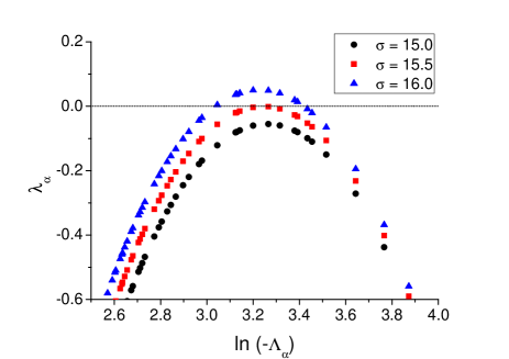
Figure 2: (Color online) Linear growth rates, $\lambda_{\alpha}$, as a function of the eigenvalues of the Laplacian, $\Lambda_{\alpha}$, for a Barabási-Albert network with $N=200$ and $\langle k\rangle=10$. In all the cases $\epsilon=0.06$ and three different values of $\sigma$ are shown for comparison. Modes with $\lambda_{\alpha}>0.0$ are observed for $\sigma>\sigma_{c}=15.5$.

IV 2 species

We first review the case of two species as a reference to the more complex patterns we study in the following sections. We consider a network with $N=1000$ nodes, constructed according to the Barabási-Albert model revbarabasi . The populations of preys, $u_{i}$, and predators, $v_{i}$, defined in each node $i$, interact locally and diffuse through the network nodes according to the equations (1), with $l=1$ (and $u_{i}^{(0)}=v_{i}^{(2)}=0$). Equations (1) are numerically integrated until a stationary distribution of the species abundance is obtained.

Figure 3 shows the stationary abundance patterns of preys, figure 3, and predators, figure 3, as a function of node index $i$, for $\epsilon=0.12$ and $\sigma=20.0$. The nodes are ordered according to decreasing degree $k_{i}$.

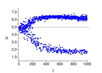
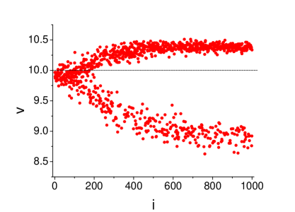
Figure 3: (Color online) Stationary abundance patterns for a single predator-prey pair as a function of node index $i$ for $\epsilon=0.12$ and $\sigma=20.0$ for (a) preys and (b) predators. The lines in $u_{i}=5.0$ and $v_{i}=10.0$ indicate the values of the homogeneous state, which is a fixed point for this set of parameters.

The pattern of prey distribution is formed by two groups of nodes presenting significant differentiation in relation to the homogeneous state: a group with high abundance (values of $u_{i}$ well above $\bar{u}$) and a group with low abundance (values of $u_{i}$ well below $\bar{u}$). The pattern of predators follows directly the pattern of the preys: nodes with large abundance of preys ($u_{i}>\bar{u}$) also have large abundance of predators ($v_{i}>\bar{v}$) and vice versa.

V 4 species

The 4 species system is described by Eq.(1) with $l=1,2$ (and $u_{i}^{(0)}=v_{i}^{(3)}=0$). The equations have a homogeneous equilibrium point that depends on the coupling parameter $\gamma$, as displayed by the table 1. The populations of preys and predators decrease as $\gamma$ increases.

$\gamma$	$u^{(1)}$	$v^{(1)}$	$u^{(2)}$	$v^{(2)}$
0.002	4.989	9.973	4.993	9.995
0.01	4.945	9.863	4.966	9.977
0.05	4.726	9.314	4.837	9.889

Table 1: Homogeneous fixed points for different values of $\gamma$ for the four species system.

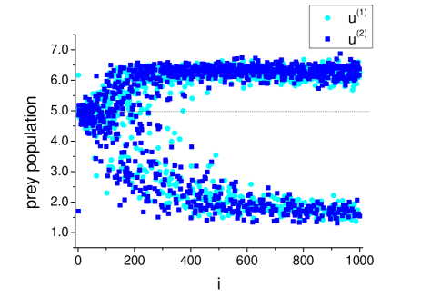
Figure 4: (Color online) Stationary abundance patterns for $u^{(1)}$ and $u^{(2)}$ as a function of node index $i$ for $\epsilon=0.12$, $\sigma=20.0$, $\phi=0.5$ and $\gamma=0.002$.

The stationary patterns of preys $u^{(1)}$ and $u^{(2)}$ as a function of the node index $i$ are shown in figure 4. These patterns of abundance (and also those of $v^{(1)}$ and $v^{(2)}$) are not very different from each other or from the previous case shown in figure 3. In particular, both types of preys and predators present the separation of nodes in high abundance and low abundance groups.

However, this similarity is partly an illusion, having to do with the way the data is plotted. Indeed, a new underlying pattern arises when difference between the prey abundances $u_{i}^{(1)}-u_{i}^{(2)}$ is plotted, as shown in figure 5 for different values of the coupling strength $\gamma$.

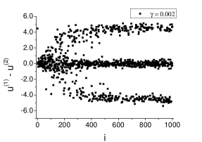
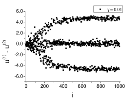
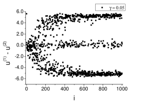
Figure 5: Stationary patterns for the difference $u^{(1)}-u^{(2)}$ as a function of node index $i$ for (a) $\gamma=0.002$, (b) $\gamma=0.01$ and (c) $\gamma=0.05$. In all cases $\epsilon=0.12$, $\sigma=20.0$ and $\phi=0.5$.

In all cases it is possible to distinguish three main branches: the upper branch, where $u^{(1)}-u^{(2)}\approx 4$, corresponding to nodes where $u^{(1)}$ is abundant but $u^{(2)}$ is not; the lower branch, where $u^{(1)}-u^{(2)}\approx-4$ where the abundances are reversed; and the middle branch, where $u^{(1)}-u^{(2)}\approx 0$ and $u^{(1)}$ and $u^{(2)}$ have similar abundances. This configuration of branches can be derived via a mean field approximation meanf1 ; meanf2 , as discussed in appendix B and displayed in Fig. 6.

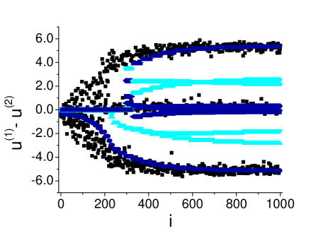
Figure 6: (Color online) Stationary pattern for the difference $u^{(1)}-u^{(2)}$ as obtained from simulations (black squares) and from the mean field approximation (blue) for $\epsilon=0.12$, $\sigma=20.0$, $\phi=0.5$ and $\gamma=0.05$. The cyan lines show unstable branches.

As $\gamma$ increases the middle branch gets less populated and the nodes are dominated mostly by a single species of prey and predator. This corresponds to a strong effect of apparent competition driven by Turing instabilities. The more important is the secondary predation (which is kept weaker than the direct predation in the each pair), the stronger is the effect.

VI 6 species

To investigate if the negative correlation between preys of coupled pairs also occur in larger trophic chains we consider a system with 6 species, again given by equation (1) with $l=1,2,3$ (and $u_{i}^{(0)}=v_{i}^{(4)}=0$). The stationary patterns of preys distributions are shown in figure 7.

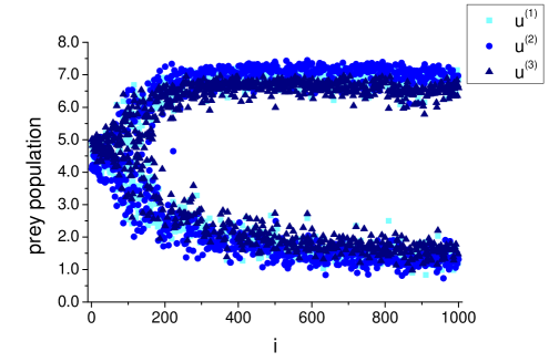
Figure 7: (Color online) Stationary patterns of preys distributions as a function of node index $i$ for the case of three pairs for $\epsilon=0.12$, $\sigma=20.0$, $\phi=0.5$ and $\gamma=0.05$.

Once again, for each prey species, the nodes cluster into groups of high and low abundances. The analysis of the correlations between different prey species, however, is now more involved. We first define the quantity:

$$\sigma_{i}^{(l)}=sng(u_{i}^{(l)}-\bar{u}^{(l)})=\left\{\begin{array}[]{rcl}+1,&\mbox{if}\ \ u_{i}^{(l)}>\bar{u}^{(l)}\\ -1,&\mbox{if}\ \ u_{i}^{(l)}<\bar{u}^{(l)}\end{array}\right.,$$ (8)

where $\sigma_{i}^{(l)}$ indicates if the $l$-th prey population at node $i$ has high ($\sigma_{i}^{(l)}=+1$) or low ($\sigma_{i}^{(l)}=-1$) abundance with respect to the homogeneous value.

Second, we separate the nodes in two groups: those with $\sigma^{(2)}=+1$ and those with $\sigma^{(2)}=-1$. Since nodes with large $k_{i}$ are not sensitive to the coupling, we restrict this analysis to nodes with $i\geq 250$, for which the differentiation is more evident. Finally we focus on the value of the sum $\sigma^{(1)}+\sigma^{(3)}$ for these nodes. The three possible values of this sum indicate the following situations: if $\sigma^{(1)}+\sigma^{(3)}=+2$, both $u^{(1)}$ and $u^{(3)}$ have high abundance in the node; if $\sigma^{(1)}+\sigma^{(3)}=-2$, both $u^{(1)}$ and $u^{(3)}$ have low abundance and if $\sigma^{(1)}+\sigma^{(3)}=0$, $u^{(1)}$ and $u^{(3)}$ have opposed abundance characteristics. If the hypothesis of negative correlation is to be valid, the group of nodes with $\sigma^{(2)}=+1$ must have most of its node with $\sigma^{(1)}+\sigma^{(3)}=-2$ and the group with $\sigma^{(2)}=-1$ must have most of its nodes with $\sigma^{(1)}+\sigma^{(3)}=+2$. The results are shown in figure 8 in the form of histograms.

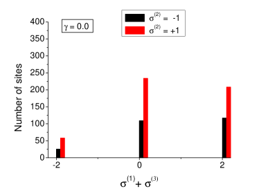
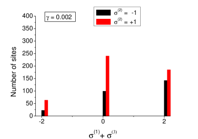
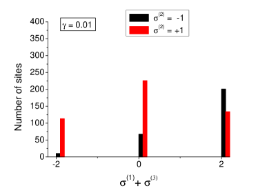
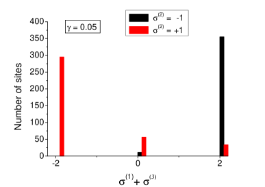
Figure 8: (Color online) Histogram of nodes with different values of $\sigma^{(1)}+\sigma^{(3)}$ for $\sigma^{(2)}=-1$ (black bars) and $\sigma^{(2)}=+1$ (red bars) for: (a) $\gamma=0.0$, (b) $\gamma=0.002$, (c) $\gamma=0.01$ and (d) $\gamma=0.05$

In Fig. 8 $\gamma=0.0$ and the three preys distributions are uncorrelated. Figures 8 and 8 display cases with increasing values of $\gamma$. As the coupling strength increases, the number of nodes with $\sigma^{(1)}+\sigma^{(3)}=+2$ increases in the group with $\sigma^{(2)}=-1$ and similarly with the number of nodes with $\sigma^{(1)}+\sigma^{(3)}=-2$ in the group where $\sigma^{(2)}=+1$. This separation is evident in figure 8, where $\gamma=0.05$, where it is clear that most of the nodes where $u^{(2)}$ has large abundance display low abundances of both $u^{(1)}$ and $u^{(3)}$ and vice versa, showing the persistence of the negative correlation between preys of coupled pairs.

VII Discussion

We have studied the formation of Turing patterns in an extended prey-predator system, considering trophic chains composed of 1, 2 and 3 prey-predator pairs, coupled by cross predation and dispersing through the connected nodes of a complex network. We detected the emergence of negative correlations between the populations of preys of coupled pairs in each node, even though there are no direct competition between preys in the equations. This effect, known in Biology as apparent competition appcomp1 ; appcomp2 , is triggered here by the Turing instabilities, and not by the local interactions.

The description of fragmented landscapes as complex networks is relatively recent in ecology fragment . Although large landscape networks have been studied minor , most of the empirical work has dealt with a relatively small number of patches urban and it is not obvious that the patterns observed here for networks with $N=1000$ nodes persist in smaller sets. We have checked that for $N$ as low as $100$ the same pattern of apparent competition can be clearly identified, but not so much for $N=50$, which seems to be a limiting size for the present set of parameters.

Another important concern in the application of our results to realist ecological problems is the topology of the network. All numerical simulations presented in the previous sections were performed for networks exhibiting power law decay of the degree distribution, that results from the application of the Barabási-Albert algorithm. Natural landscape networks can exhibit significant heterogeneity in the degree distribution fortuna , but are not necessarily scale free. In order to verify the robustness of our results against changes in the network topology we have also simulated networks with Poisson degree distribution, associated to random networks. We found that the negative correlations between preys still holds for $N=1000$ and average degree $\langle k\rangle=20$.

The occurrence of Turing patterns in real ecological systems is still an open question. This is in part due to the difficulties in conducting controlled ecological field experiments to distinguish between patterns related to space heterogeneity or to intrinsic mechanisms of the interaction. However, there is growing evidence of species distribution patterns formed by the Turing mechanism rietker ; maron .

Our results point to the possibility that, at least in part, species abundance patterns might be related to Turing instabilities and not to environmental heterogeneity. Moreover, strong effects of apparent competition might emerge spontaneously as Turing patterns, resulting from diffusion instabilities and not necessarily from local interactions.

VIII Aknowledgements

It is a pleasure to thank Carolina Reigada for important discussions. This work was partly supported by FAPESP and CNPq.

Appendix A Critical value for Turing instability

The eigenvalues of the Jacobian matrix of 7 are given by the roots of the characteristic polinomial

$$\lambda_{\alpha}^{2}-\lambda_{\alpha}(f_{u}+g_{v}+(1+\sigma)\varepsilon\varLambda_{\alpha})+(f_{u}+\varepsilon\varLambda_{\alpha})(g_{v}+\sigma\varepsilon\varLambda_{\alpha})-f_{v}g_{u}=0$$

which are given by

$$\lambda_{\alpha}=\frac{f_{u}+g_{v}+(1+\sigma)\varepsilon\varLambda_{\alpha}\pm\sqrt{4f_{v}g_{u}+(f_{u}-g_{v}+(1-\sigma)\varepsilon\varLambda_{\alpha})^{2}}}{2}.$$ (9)

For each mode $\alpha$ there are two possible values for $\lambda_{\alpha}$, but only the one associated to the plus sign can become positive, so we only need to consider this eigenvalue. Solving $d(\lambda_{\alpha})/d(\varLambda_{\alpha})=0$ we obtain the critical Laplacian eigenvalue. Substituting this value in 9 and imposing that $Re(\lambda_{\alpha_{c}})=0$ in the instability threshold, we obtain the critical value $\sigma_{c}$:

$$\sigma_{c}=\displaystyle\frac{f_{u}g_{v}-2f_{v}g_{u}+2\sqrt{f_{v}g_{u}(f_{v}g_{u}-f_{u}g_{v})}}{f_{u}^{2}}.$$ (10)

Appendix B Mean field approximation

The mean field approximation consists in averaging the heterogeneous degree distribution of the network by adjusting the strength by which each node senses the presence of its neighbors. Introducing the local fields

$$\begin{array}[]{cc}x_{i}^{l}=\sum_{j=1}^{N}A_{ij}u_{j}^{(l)}\\ y_{i}^{l}=\sum_{j=1}^{N}A_{ij}v_{j}^{(l)}\end{array}$$ (11)

and substituting in Eq.(1), we obtain

$$\frac{d}{dt}u_{i}^{(l)}(t) =f(u_{i}^{(l)},v_{i}^{(l)})-\gamma u_{i}^{(l)}v_{i}^{(l+1)}+\varepsilon\left(x_{i}^{l}-k_{i}u_{i}^{(l)}\right)$$

$$\frac{d}{dt}v_{i}^{(l)}(t) =g(u_{i}^{(l)},v_{i}^{(l)})+\phi\gamma u_{i}^{(l-1)}v_{i}^{(l)}+\sigma\varepsilon\left(y_{i}^{l}-k_{i}v_{i}^{(l)}\right).$$ (12)

We then consider the approximations $x_{i}^{l}\simeq k_{i}X^{l}$ and $y_{i}^{l}\simeq k_{i}Y^{l}$, where the global fields $X$ and $Y$ are defined as the weighted averages

$$\begin{array}[]{cc}X^{l}=\sum_{j=1}^{N}w_{j}u_{i}^{(l)}\\ Y^{l}=\sum_{j=1}^{N}w_{j}v_{i}^{(l)}\end{array}$$ (13)

with the weights

$$w_{j}=k_{j}\big{/}\sum_{l=1}^{N}k_{l}.$$ (14)

This choice gives hubs have a stronger influence in the calculation of the global fields.

With this approximation, and introducing the parameter $\beta(i)=\varepsilon k_{i}$, the dynamical system may be written as:

$$\frac{d}{dt}u^{(l)}(t) =f(u^{(l)},v^{(l)})-\gamma u^{(l)}v^{(l+1)}+\beta\left(X^{l}-u^{(l)}\right)$$

$$\frac{d}{dt}v^{(l)}(t) =g(u^{(l)},v^{(l)})+\phi\gamma u^{(l-1)}v^{(l)}+\sigma\beta\left(Y^{l}-v^{(l)}\right),$$ (15)

where each dynamical variable interacts only with its associated global field. Since every node now possesses the same dynamical equation, we may drop the index $i$.

In order to describe the patterns for the difference of prey populations, in the case with 2 prey-predator pairs, we define the new variables:

$$\begin{array}[]{cccc}u_{\pm}=u^{(1)}\pm u^{(2)}\\ v_{\pm}=v^{(1)}\pm v^{(2)}\end{array}$$ (16)

The system of equations (15), written with the new variables (16), is given by:

$$\frac{du_{\pm}}{dt} =F_{\pm}(u_{-},u_{+},v_{-},v_{+})-\frac{\gamma}{4}(u_{-}+u_{+})(v_{+}-v_{-})+\beta\left(X^{\pm}-u_{+}\right)$$

$$\frac{dv_{\pm}}{dt} =G_{\pm}(u_{-},u_{+},v_{-},v_{+})\pm\frac{\phi\gamma}{4}(u_{-}+u_{+})(v_{+}-v_{-})+\sigma\beta\left(Y^{\pm}-v_{+}\right),$$ (17)

where

$$\begin{array}[]{cccc}F_{\pm}=f(u^{(1)}(u_{-},u_{+}),v^{(1)}(v_{-},v_{+}))\pm f(u^{(2)}(u_{-},u_{+}),v^{(2)}(v_{-},v_{+}))\\ G_{\pm}=g(u^{(1)}(u_{-},u_{+}),v^{(1)}(v_{-},v_{+}))\pm g(u^{(2)}(u_{-},u_{+}),v^{(2)}(v_{-},v_{+}))\end{array}$$ (18)

and

$$\begin{array}[]{cccc}X^{\pm}=X^{1}\pm X^{2}\\ Y^{\pm}=Y^{1}\pm Y^{2}\\ \end{array}$$ (19)

If the global fields for each dynamical variable are given, the parameter $\beta$ may be seen as a bifurcation parameter. It is possible to note a saddle node bifurcation in the system, and the appearance of new stable fixed points, when the value of $\beta$ is increased from $\beta=0$.

We obtain the global fields (19) by numerically integrating equations (1) and using the stationary values of the dynamical variables in (13) and these in (19). We then construct bifurcation diagrams calculating, for each value of $\beta$, the fixed points of the system (17). Since each node has an associated degree $k_{i}$, and, therefore, an associated $\beta$, it is possible to project the bifurcation diagram in the stationary pattern that resulted of the numerical integration of (1). The projection of the bifurcation diagram relative to the variable $u_{-}$ on the stationary pattern for the difference $u^{(1)}-u^{(2)}$ is shown in figure 6.

References

- (1) J. Murray, Mathematical Biology I: An Introduction (Springer, New York, 2002).
- (2) J. Murray, Mathematical Biology II: Spatial Models and Biomedical Applications (Springer, New York, 2003).
- (3) A.M. Turing, Philosophical Transactions of the Royal Society of London. Series B, Biological Sciences, 237, 37 (1952).
- (4) J. Murray, Journal of Theoretical Biology, 98, 143 (1982).
- (5) J. Murray, Scientific American, 258, 80 (1988).
- (6) M. Mimura and J. Murray, Journal of Theoretical Biology, 75, 249 (1978).
- (7) A. Koch and H. Meinhardt, Reviews of Modern Physics, 66, 1481 (1994).
- (8) K. Kishimoto, Journal of Mathematical Biology, 16, 103 (1982).
- (9) M. Baurmann, T. Gross and U. Feudel Journal of Theoretical Biology, 245, 220 (2007).
- (10) T. Bánsági Jr, V. K. Vanag and I. R. Epstein, Science, 331, 1309 (2011).
- (11) M. Yamaguchi, E. Yoshimoto and S. Kondo, Proceedings of the National Academy of Sciences USA, 104, 4790 (2007).
- (12) S. Sawai, Y. Maeda and Y. Sawada, Physical Review Letters, 85, 2212 (2000).
- (13) H. Nakao and A. S. Mikhailov, Nature Physics, 6, 544 (2010).
- (14) R. Albert and A-L. Barabási, Reviews of Modern Physics, 74 (1), 47 (2002).
- (15) M. Hagen, W.D. Kissling, C. Rasmussen, M.A.M. de Aguiar, L.E. Brown, D.W. Carstensen et al. Advances in Ecological Research, 46 (2012) in press
- (16) M.A. Fortuna, C. Gómez-Rodríguez and J. Bascompte, Proceedings of the Royal Society B, 273, 1429 (2006).
- (17) M. Rietker and J. van de Koppel, Trends in Ecology and Evolution, 23 (3), 169 (2008).
- (18) J. Maron and S. Harrison Science, 278, 1619 (1997).
- (19) F. Courchamp, T. Clutton-Brock and B. Grenfell, Trends in Ecology and Evolution, 14 (10), 405 (1999).
- (20) P. Stephens and W. Sutherland, Trends in Ecology and Evolution, 14 (10), 401 (1999).
- (21) M. Begon, C. Townsend and J. Harper, Ecology: From Individuals to Ecosystems (Wiley-Blackwell, Oxford, 2006).
- (22) T. Ichinomiya, Physical Review E, 70, 026116 (2004).
- (23) H. Nakao and A. S. Mikhailov, Physical Review E, 79, 036214 (2009).
- (24) R. Holt and R. Lawton, Annual Review of Ecology and Systematics, 25, 495 (1994).
- (25) E. Chaneton and M. Bonsall Oikos, 88, 380 (2000).
- (26) E. S. Minor and D. L. Urban, Conservation Biology, 22, 297 (2008).
- (27) D. Urban and T. Keitt, Ecology, 82, 1205 (2001).