Dynamic shear responses of polymer-polymer interfaces

Abstract

In multi-component soft matter, interface properties often play a key role in determining the properties of the overall system. The identification of the internal dynamic structures in non-equilibrium situations requires the interface rheology to be characterized. We have developed a method to quantify the rheological contribution of soft interfaces and evaluate the dynamic modulus of the interface. This method reveals that the dynamic shear responses of interfaces in bilayer systems comprising polypropylene and three different polyethylenes can be classified as having hardening and softening effects on the overall system: a interface between linear long polymers becomes more elastic than the component polymers, while large polydispersity or long-chain-branching of one component make the interface more viscous. We find that the chain lengths and architectures of the component polymers, rather than equilibrium immiscibility, play an essential role in determining the interface rheological properties.

I Introduction

The rheological properties of emulsions or blends of immiscible materials have been the subject of much research. The physical properties of such multi-component complexes are not only a simple average of the properties of the components but also depend on the morphological structure and interface properties. Many studies have addressed the relationship between morphology and rheological properties.Sperling1997Polymeric ; Robeson2007Polymer In contrast, the rheological properties of an interface are still not fully understood.

Regarding the extrusion instability of a polymer melt, slippage at a polymer–wall interface has received much attention.Brochard1992Sheardependent ; Munstedt2000Stick ; Denn2001EXTRUSION ; Migler1993Slip ; Park2008Wall In contrast, slippage at a polymer–polymer interface was introduced to explain the anomalously low viscosity in immiscible polymer blends.ChenChongLin1979Mathematical ; LyngaaeJorgensen1988Influence Considering shear flow parallel to the flat interface between two polymers, the viscosity of this bilayer system under the stick boundary condition, $\eta^{\text{st}}$, becomes the harmonic mean of the viscosities of the components, $\eta_{1}$ and $\eta_{2}$:

$$\frac{1}{\eta^{\text{st}}} =\sum_{\alpha=1,2}\frac{\phi_{\alpha}}{\eta_{\alpha}},$$ (1)

where $\phi_{\alpha}$ is the volume fraction of the polymer $\alpha$. Lin defined the ratio of the stick viscosity to the measured viscosity, $\eta$, to characterize the slip: $\beta=\eta^{\text{st}}/\eta$.ChenChongLin1979Mathematical The physical origin of the partial slip of $\beta>1$ was attributed to the viscosity of the interfacial layer, $\eta_{I}$, by Lyngaae-Jørgensen et al.LyngaaeJorgensen1988Influence as

$$\frac{1}{\eta} =\sum_{\alpha=1,2}\frac{\phi_{\alpha}}{\eta_{\alpha}}+\frac{\phi_{I}}{\eta_{I}},$$ (2)

where $\phi_{I}$ is the volume fraction of the interfacial layer. Rewriting Eq. (2) with $\beta$ under the thin-interface limit of $\phi_{I}\to 0$ gives the ratio of the bilayer viscosity to the interface viscosity, $1-1/\beta=\eta\phi_{I}/\eta_{I}$. Let the interface thickness be $h_{I}$; the slip velocity of the interface, $\Delta V_{I}=h_{I}\dot{\gamma}_{I}$, can be defined to be finite even under the thin-interface limit of $h_{I}\to 0$. In a bilayer system with the thickness $h_{W}$, let the shear stress be $\tau$ and the apparent shear rate of the bilayer be $\dot{\gamma}_{W}$. We have the relation $\eta\phi_{I}/\eta_{I}=\dot{\gamma}_{I}h_{I}\tau/(\dot{\gamma}_{W}h_{W}\tau)=\Delta V_{I}/\Delta V_{W}$, where $\Delta V_{W}$ is the relative velocity between both surfaces of the bilayer. Lam et al. redefined the degree of slip as $\varphi=1-1/\beta=\Delta V_{I}/\Delta V_{W}$, which they called the energy dissipation factor in relation to the contribution of the interface to the total energy dissipation of the bilayer system.Lam2003Interfacial_properties Along with the energy dissipation factor, another slip index $\phi_{I}\gamma_{I}/\gamma_{W}$ under oscillatory shear deformation parallel to the interface was usedJiang2005Rheological , where $\gamma_{I}$ and $\gamma_{W}$ are the strain amplitudes of the interface layer and the entire bilayer, respectively. The existence of the slippage at different polymer–polymer interfaces have been reported by observing non-zero $\varphi$.Lam2003Interfacial_properties ; Jiang2005Rheological ; Lam2003Interfacial ; Jiang2003Energy

The slip velocity’s onset and dependence on the shear stress have also been studied.Migler2001Visualizing ; Zhao2002Slip ; lee09:_polym_polym_inter_slip_in_multil_films ; Park2010Polymerpolymer These studies focused on the slip at rather high shear rate. The sigmoidal dependence of $\Delta V_{I}$ on $\tau$ and power-law regimes of $\Delta V_{I}\propto\tau^{n}$ were observed in different polymer–polymer interfaces, and the exponent $n$ depends on pairs. The differences in exponents might be related to the miscibility, molecular weight distributions and entanglement structures of the components, but this matter still requires more systematic studies.

A polymer–polymer interface has a small but finite thickness.Jones1999Polymers Thus, different conformations from the bulk in a certain region around an interface may induce different relaxations, i.e., different viscoelastic properties. From this viewpoint, the slip velocity under steady shear determines the viscous property of the interface. For bulk polymers, the dynamic response reflects the internal structure of a material; therefore, rheological measurements are used to assess structural information.dealy06:_struc_and_rheol_of_molten_polym Thus, the dynamic response of a polymer–polymer interface can be used as a probe of the interface structure.

An attempt to measure the dynamic modulus of polymer–polymer interfaces was reported. Song and DaiSong2010TwoParticle applied a passive microrheology technique to an interface between polydimethylsiloxane and polyethylene glycol using Pickering emulsions at room temperature. In this technique, a tracer particle is confined to the interface region by physico-chemical absorption.

In this article, we developed a method to evaluate the dynamic modulus of a polymer–polymer interface in the linear-response regime. To form an interface for study, bilayer samples of immiscible polymers were prepared. From independent dynamic measurements of a bilayer and its component polymers, the dynamic modulus of an interface was evaluated. This technique was applied to interfaces between polypropylene and different polyethylenes with different chain architectures and molecular weight distributions.

II Interfacial boundary layer and its dynamic modulus

We consider a system with two immiscible polymers melts A and B having a macroscopically flat interface. In equilibrium, the interface between the two immiscible polymers has a small but finite thickness of $a_{I}$.Jones1999Polymers

To discuss the dynamic response of the interface, we apply an oscillatory shear stress

$$\tau(\omega,\tau_{0}) =\tau_{0}e^{i\omega t},$$ (3)

parallel to the interface on the polymer A and measure a response strain of the overall bilayer system, $\gamma_{W}$. In this measurement, the applied stress on the polymer A is transmitted to the polymer B through the interface. It is assumed that a region around the interface exists whose response strain, $\gamma_{I}$, to the applied shear stress is different from those of the A and B bulk layers, $\gamma_{A}$ and $\gamma_{B}$. We call this region the interfacial boundary layer (Fig. 1). The thickness of the interfacial boundary layer $h_{I}$, which is defined under non-equilibrium steady state, may be different from the equilibrium thickness $a_{I}$, which is determined thermodynamically by the free energy of the entire bilayer system.

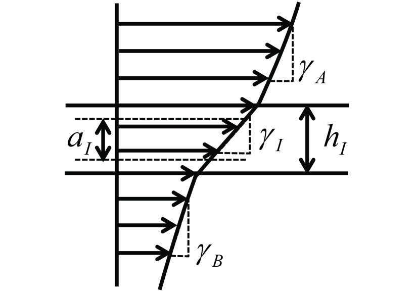
Figure 1: Schematic of the displacement across an interfacial boundary layer.

Similarly, a layer deforming with the strain response of the bulk polymer A(B), $\gamma_{A}$($\gamma_{B}$), is called the layer A(B). The thickness of the layer A(B) is denoted as $h_{A}$($h_{B}$). Therefore, the thickness of the overall system is $h_{W}=h_{A}+h_{I}+h_{B}$.

We then define the thickness fraction as

$$c_{\alpha} =\frac{h_{\alpha}}{h_{W}},~{}~{}(\alpha=A,B,I)$$ (4)

where the relation $1=\sum_{\alpha=A,B,I}c_{\alpha}$ holds. With these thickness fractions, the apparent deformation $\gamma_{W}$ of the overall system is expressed as

$$\gamma_{W} =\sum_{\alpha=A,B,I}\gamma_{\alpha}c_{\alpha},$$ (5)

We note that, although the thickness of the interfacial boundary layer is supposed to be much smaller than those of the bulk layers ($c_{I}\ll c_{A},c_{B}$), the deformation of the interfacial boundary layer can be comparable to those of the bulk layers. Suppose that $\gamma_{I}\approx\gamma_{A},\gamma_{B}$. The contribution of the interfacial boundary layer to the total strain is much smaller than those of the bulk layers due to the small thickness of the interfacial boundary layer, i.e., $c_{I}\gamma_{I}\ll c_{A}\gamma_{A},c_{B}\gamma_{B}$ and is therefore barely detectable macroscopically. In this case, the interface would be referred to as macroscopically stick. In contrast, suppose that $c_{I}\gamma_{I}\gtrsim c_{A}\gamma_{A},c_{B}\gamma_{B}$, where the deformation of the interfacial boundary layer is comparable to that of the bulk layers. In this case, the interface would be referred to as macroscopically non-stick or slip.

We are ready to consider the dynamic modulus of each layer. The time-dependent strain of the $\alpha$th layer is written as $\gamma_{\alpha}=\gamma_{\alpha,0}e^{i\omega t}$ with a time-independent amplitude $\gamma_{\alpha,0}$. The complex modulus of the $\alpha$th layer in the linear response regime, $G_{\alpha}^{*}(\omega)$, is defined as

$$\tau =G_{\alpha}^{*}\gamma_{\alpha,0}e^{i\omega t},$$ (6)

$$G_{\alpha}^{*} =\left|G_{\alpha}^{*}\right|e^{i\delta_{\alpha}}=G_{\alpha}^{{}^{\prime}}+iG_{\alpha}^{{}^{\prime\prime}},$$ (7)

where $G^{\prime}_{\alpha}$, $G^{\prime\prime}_{\alpha}$, and $\delta_{\alpha}$ are the storage modulus, loss modulus, and phase lag of the $\alpha$th layer, respectively. Combining Eqs. (5) and (6) yields

$$\frac{G_{I}^{*}}{c_{I}} =\left[\frac{1}{G_{W}^{*}}-\sum_{\alpha=A,B}\frac{c_{\alpha}}{G_{\alpha}^{*}}\right]^{-1},$$ (8)

which is the dynamic modulus of the interfacial boundary layer up to the interface thickness fraction. Let

$$D_{s}-iD_{L} =\frac{1}{G_{W}^{*}}-\sum_{\alpha=A,B}\frac{c_{\alpha}}{G_{\alpha}^{*}},$$ (9)

then the amplitude and the phase lag of the interface dynamic modulus are expressed as

$$\frac{\left|G_{I}^{*}\right|}{c_{I}} =\frac{1}{\sqrt{D_{S}^{2}+D_{L}^{2}}},$$ (10)

$$\tan\delta_{I} =\frac{D_{L}}{D_{S}}.$$ (11)

$D_{S}$ and $D_{L}$ are determined by $G_{W}^{*}$, $G_{A}^{*}$ , $G_{B}^{*}$, $c_{A}$ and $c_{B}$. Henceforth, Eqs. (10) and (11) are used to determine the dynamic modulus of the interfacial boundary layer up to $c_{I}$. Note that the phase lag of the interfacial boundary layer can be determined independently of $c_{I}$.

III Assessment of the interfacial contribution to the overall bilayer system

To obtain the dynamic modulus of the interfacial boundary layer, the thickness fractions, $c_{A}$ and $c_{B}$ , in addition to the moduli $G_{W}^{*}$, $G_{A}^{*}$, and $G_{B}^{*}$, are required. In this section, we introduce a method of assessing the presence and extent of the rheological contribution of the interface to the overall bilayer system solely from the moduli $G_{W}^{*}$, $G_{A}^{*}$, and $G_{B}^{*}$.

Assume that no interfacial boundary layer exists under shear such that the interface exhibits a completely stick response. In this case, the modulus of the overall system can be completely determined by those of the bulk layers of the polymers A and B. Equation (8) is reduced to

$$\frac{e^{-i\delta_{W}}}{\left|G_{W}^{*}\right|} =\sum_{k=A,B}c_{k}\frac{e^{-i\delta_{k}}}{\left|G_{k}^{*}\right|}.$$ (12)

We note that this relation (12) can be regarded as a linear simultaneous equation with two unknowns $c_{A}$ and $c_{B}$ for given $G_{W}^{*}$, $G_{A}^{*}$, and $G_{B}^{*}$. Let $c_{A}^{\text{st}}$ and $c_{B}^{\text{st}}$ be the solutions of Eq. (12). If the assumption of the stick interface, namely no interface contribution, is valid, the relation $c_{A}^{\text{st}}+c_{B}^{\text{st}}=1$ is expected. On the contrary, if an interfacial contribution exists, this effect is reflected in $c_{A}^{\text{st}}+c_{B}^{\text{st}}\neq 1$. From this observation, we define a measure of the interface contribution by $c_{I}^{\text{ns}}=c_{A}^{\text{st}}+c_{B}^{\text{st}}-1$, which we call the non-stick degree of interface.

To understand the physical implication of $c_{I}^{\text{ns}}$, we consider a model case of two immiscible polymers with the same modulus $G_{A}^{*}=G_{B}^{*}$. For simplicity, we assume that $\delta_{W}=\delta_{A}$. In this case, Eq. (12) reduces to

$$\frac{\left|G_{A}^{*}\right|}{\left|G_{W}^{*}\right|} =c_{A}^{\text{st}}+c_{B}^{\text{st}}=1+c_{I}^{ns}.$$ (13)

When the interface is stick, $\left|G_{W}^{*}\right|=\left|G_{A}^{*}\right|$ implies that $c_{I}^{\text{ns}}=0$. When the interface is non-stick, both positive and negative $c_{I}^{\text{ns}}$ are possible. A positive $c_{I}^{\text{ns}}$ implies that $\left|G_{W}^{*}\right|<\left|G_{A}^{*}\right|$, which means that the bilayer is softened due to the existence of the interfacial boundary layer (Fig. 2). In this case, the excess length of $h_{W}c_{I}^{\text{ns}}$ is a counterpart of the slip length, $l=\Delta V_{I}/\dot{\gamma}$, in slippage under steady shear. gennes79:_viscom_flows_of_tangl_polym Conversely, a negative $c_{I}^{\text{ns}}$ implies that $\left|G_{W}^{*}\right|>\left|G_{A}^{*}\right|$, which means that the bilayer is hardened due to the existence of the interfacial boundary layer (Fig. 3). In this case, to explain the apparent strain of the bilayer system, $\gamma_{W}$, solely from the strains $\gamma_{A}$ and $\gamma_{B}$, a finite interfacial boundary layer is required; a layer with a finite thickness of $h_{W}\left|c_{I}^{\text{ns}}\right|$ has zero strain. For the interface modulus to be finite, a thickness of the interfacial boundary layer $h_{I}>h_{W}\left|c_{I}^{\text{ns}}\right|$ is implied. In other words, $h_{W}\left|c_{I}^{\text{ns}}\right|$ gives a lower limit for the thickness of the interfacial boundary layer.

In general, a nonzero $c_{I}^{\text{ns}}$ implies the existence of an interface contribution to the bilayer modulus. Moreover, the different sign of $c_{I}^{\text{ns}}$ reflects a different qualitative contribution of the interface to the bilayer modulus.

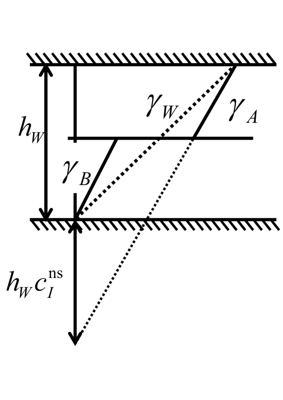
Figure 2: Schematic illustration of displacement for a negative non-stick degree of interface, $c_{I}^{\text{ns}}>0$. To explain the apparent strain for the bilayer system $\gamma_{W}$ from the strains $\gamma_{A}$ and $\gamma_{B}$, large strain at the thin interface is implied.

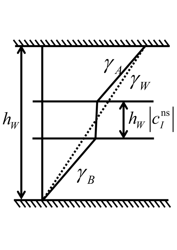
Figure 3: Schematic illustration of displacement for a positive non-stick degree of interface, $c_{I}^{\text{ns}}<0$. To explain the apparent strain of the bilayer system $\gamma_{W}$ from the strains $\gamma_{A}$ and $\gamma_{B}$, a finite interfacial boundary layer with a small strain is implied.

IV Experimental

IV.1 Materials

The polymers used in this study are listed in Table 1. Three different polyethylenes were obtained from the Japan Polyethylene Corporation: linear low-density polyethylene (LLDPE)( NOVATEC™-LL(UJ960)), high-density polyethylene (HDPE)( NOVATEC™-HD(HJ362N)), and low-density polyethylene (LDPE)( NOVATEC™-LD(LF640MA)). Polypropylene (PP) was obtained from the Japan Polypropylene Corporation (NOVATEC™-PP (BC4BSW)) The molecular weight distributions of LLDPE, HDPE, and PP were estimated from their melt dynamic moduli by an algorithm developed by Mead.Mead1994Determination This method has been implemented in Rheometric Scientific’s Orchestrator software of TA instruments. The Mead’s algorithm is based on theory for a linear polymer and cannot be used for a polymer with long-chain-branching. The weight-averaged molecular weight, $M_{w}$, and polydispersity, $M_{w}/M_{n}$, of LDPE was supplied by the manufacturer. The polymers were in pellet form. The melting point, $T_{m}$, and thermal decomposition temperature were obtained through thermogravimetry and differential thermal analysis in air.

Table 1: Characteristics of the polymer samples. Molecular weight distributions estimated from the melt dynamic moduli by an algorithm developed by Mead.Mead1994Determination , with the exception of LDPE, for which the manufacturer supplied the information.

polymer	$M_{w}$(kg/mol)	$M_{w}/M_{n}$	$T_{m}$(∘C)	$T_{d}$(∘C)
polyethylene
LLDPE	71.2	4.49	127	232
HDPE	70.4	13.3	132	220
LDPE	65	3.82	114	229
polypropylene
PP	155	9.85	168	236

IV.2 Sample Preparation

Polymer pellets were dried for at least 24 h at 100^∘C in a vacuum oven prior to use. Each polymer was compression-molded at a temperature of approximately 60^∘C above each melting point in a hot press to form a plaque and then cooled to room temperature. The thickness of each polymer plaque was kept at approximately 1 mm using a spacer frame made of stainless steel so that the plaque was suitable for the rheological measurements described below. Each polymer melt was pressed between two sheets of polytetrafluoroethylene (Naflon™PTFE from NICHIAS Corporation).

IV.3 Rheological measurements

We focused on pairs of polypropylene and different polyethylenes, namely PP/LLDPE, PP/LDPE, and PP/HDPE bilayer systems.

For both pure polymers and bilayers, the dynamic shear moduli were measured in parallel-plate geometry with a plate diameter of 25 mm in a rheometer (Rheometric Dynamic Analyzer II , TA instruments) at different temperatures under a nitrogen atmosphere. The measurement was performed within the frequency range 0.1-$5\times 10^{2}$ rad/s. The strain amplitude was set at approximately 10% or lower, which corresponded to the linear response regime in all of the pure polymers and bilayers, as identified through preliminary amplitude sweeps.

Bilayer samples were prepared in the sample chamber of the rheometer. We loaded two different polymer plaques in the sample chamber and raised the chamber temperature to a given measurement temperature to melt the polymers. At the measurement temperature, the gap between the parallel plates was compressed to approximately 2 mm. We note that the thicknesses of two polymers in a bilayer at a given measurement temperature differ because of the difference in each polymer’s thermal expansion. To equilibrate the polymer-polymer interface, we held the bilayer at the measurement temperatures for 30 min. Subsequently, dynamic measurements were obtained.

Thickness fractions for each bilayer at a given measurement temperature were computed from a digital photograph of the sample chamber up to two decimal places.

V Results and Discussion

V.1 Linear dynamic moduli and chain architectures of the pure polymers

Frequency-sweep measurements were made for each polymer listed in Table 1 at different temperatures between $T_{m}$ and $T_{d}$: 180, 190, and 220^∘Cfor PP and 140, 190, and 220^∘Cfor LLDPE, LDPE, and HDPE, respectively. Figure 4 shows the linear dynamic modulus of each polymer in the form of a van Gurp–Palmen plot (phase lag versus absolute value of the complex modulus).

Figure 4: The van Gurp–Palmen plots of the pure polymers at a reference temperature of 190^∘C.

In the van Gurp–Palmen plot, the frequency is eliminated to examine the applicability of time-temperature superposition. Figure 4 shows that for all the pure polymers, a master curve was obtained by applying both frequency shift and amplitude shift.

Next, we consider the chain architectures of the pure polymers. It was reported that the van Gurp–Palmen curves had shapes specific to the different chain architectures dealy06:_struc_and_rheol_of_molten_polym ; Lohse2002WellDefined ; Trinkle2002Van ; schlatter05:_fourier_trans_rheol_branc_polyet ; VictorHugoRolonGarrido2007Molecular ; Malmberg2002LongChain . Although the frequency range was limited in our measurements, the van Gurp–Palmen curves of the pure polymers in Fig. 4 exhibited different characteristic shapes. For PP and LLDPE, the curves started from nearly $\delta=90^{\circ}$ and exhibited cap-convex shapes, which are characteristic of linear polymers. For LDPE, the curves also started from nearly $\delta=90^{\circ}$ but decreased more rapidly than a linear polymer and had a cup-convex shape, which is characteristic of the long-chain-branching of densely branched polymers. For HDPE, the curves started from $\delta\approx 70^{\circ}$ and had a lower $\delta$ than LLDPE, which manifested a higher elasticity than LLDPE. The difference in the van Gurp–Palmen curves of HDPE and LLDPE might be explained by the difference in polydispersity and/or a possible difference in chain architectures. The higher the degree of polydispersity, the more the van Gurp–Palmen curve is stretched at low modulus.Trinkle2001Van The large value of $M_{w}/M_{n}=13.3$ for HDPE seems to explain in part the van Gurp–Palmen curve for HDPE. However, the smaller $\delta$ in the low-modulus region is still far from the curves of linear chains. This characteristic was similar to the curves of the long-chain-branching of sparsely branched polymers ($<$1 branch per chain). Trinkle2002Van ; schlatter05:_fourier_trans_rheol_branc_polyet To summarize these observations, the three polyethylenes used in this study were inferred to have different chain architectures: linear (LLDPE), densely branched (LDPE), and sparsely branched (HDPE) architectures.

V.2 Linear dynamic moduli of bilayers and non-stick degrees of interfaces

The linear moduli of polypropylene and polyethylene bilayers are depicted in Figs. 5, 6, and 7. The modulus amplitude and phase lag of the PP/LLDPE bilayer lies between those of pure PP and LLDPE  (Fig. 5). At a glance, the dynamic modulus of the PP/LLDPE bilayer appears to be an average of those of the component polymers. However, even for this case, some interface contribution was detected, as described below. Unlike PP/LLDPE, the bilayer modulus of PP/LDPE was close to that of LDPE (Fig. 6). This result implies that the PP/LDPE bilayer was softer than the average of the component polymers due to an interface effect. More distinct softening was observed in PP/HDPE bilayer (Fig. 7). The bilayer modulus of PP/HDPE was lower than those of the component polymers. Moreover, a larger phase lag of the PP/HDPE bilayer than those of the component polymers occurred in a certain frequency range. This observation in the PP/HDPE bilayer also implies an interface effect.

Figure 5: Amplitude of the complex modulus and phase lag for PP, LLDPE, PP/LLDPE bilayer, and PP/LLDPE interface at 190^∘C.

Figure 6: Amplitude of the complex modulus and phase lag for PP, LDPE, PP/LDPE bilayer, and PP/LDPE interface at 190^∘C.

Figure 7: Amplitude of the complex modulus and phase lag for PP, HDPE, PP/HDPE bilayer, and PP/HDPE interface at 190^∘C.

We now evaluate the non-stick degrees of the interfaces between polypropylene and different polyethylenes. For the measured moduli of a bilayer and its two component polymers at a given frequency, $(c_{A}^{\text{st}},c_{B}^{\text{st}})$ are obtained by solving Eq. (12). By definition, $c_{I}^{\text{ns}}$ might depend on frequency. However, the sign of $c_{I}^{\text{ns}}$ would be insensitive to frequency because the softness or hardness of an interface is qualitatively determined by the pair of polymers. Therefore, we focus on one representative $c_{I}^{ns}$ for each pair. From a technical viewpoint, we computed $c_{I}^{ns}$ at a frequency at which the condition number of the matrix in Eq. (13) is minimum and where $c_{I}^{ns}$ is least affected by the measurement error of $G_{I}^{*}$.

The non-stick degrees $c_{I}^{\text{ns}}$ were -0.023 for the PP/LLDPE interface, 0.17 for the PP/LDPE interface, and 0.32 for the PP/HDPE interface. This result revealed that each interface contributed to the dynamic response of each bilayer at a certain level in all the pairs of the polypropylene and polyethylenes. Depending on the sign of $c_{I}^{\text{ns}}$, the interfaces are classified into two groups. The positive $c_{I}^{\text{ns}}$ for PP/LDPE and PP/HDPE showed that these bilayers had a softer dynamic response than the averages of the components. In contrast, the negative $c_{I}^{\text{ns}}$ for PP/LLDPE indicated a hardening contribution of the interface to the dynamic response of the bilayer.

The three polyethylenes used were similar in weight-averaged molecular weights but differed in molecular weight distribution and chain architecture. The difference in the responses of the interfaces indicated that the dynamical structure of an interfacial boundary layer depended on the chain structure rather than solely on the miscibility. It is presumed that a substantial chain component comprising an interface differs depending on the chain structures.

In the PP/LLDPE bilayer, both PP and LLDPE are entangled linear chains. In this case, the chains comprising the interface can have a number of entanglement points. This entanglement would make the PP/LLDPE interfacial boundary layer hard. In contrast, HDPE has a larger polydispersity than LLDPE, indicating that HDPE has a certain proportion of shorter chains. Short chains are more likely to be near the interface than in the bulk. Therefore, at the PP/HDPE interface, the number of entanglement points would be less than at the PP/LLDPE interface, which would make the PP/HDPE interface boundary layer soft.

In the case of a long-chain-branching LDPE, the PP/LDPE interface also showed a softening behavior. This fact indicates that short side chains mainly contributed to the interface structure. Densely branched chains are less likely to diffuse into the interfacial layer. Thus, backbone chains would tend to be in the bulk. This feature could be a possible cause of a softening contribution of the PP/LDPE interface. The $c_{I}^{\text{ns}}$ for the PP/LDPE interface was smaller than that for the PP/HDPE interface. This difference would be due to the lower mobility of a densely branched chain.

These results suggest that chain lengths and chain architectures are responsible for the dynamic response of an interface. Equilibrium miscibility is not sufficient to predict the dynamic response of an interface.

V.3 Dynamic modulus of interface

We now consider the dynamic moduli of interfaces between the polypropylene and different polyethylenes. To compute $G_{I}^{*}$ by Eqs. (10) and (11), the thickness fractions of the bulk layers A and B and the interfacial boundary layer are required. The thicknesses of the layers A and B at a given measurement temperature were estimated from the digital image of a bilayer sample in the chamber. However, the thickness of an interfacial boundary layer $h_{I}$ is not known a priori. For the softening interfaces of PP/LDPE and PP/HDPE, we assume that $h_{I}$ is of the same order of magnitude as the equilibrium thickness of an interface $a_{I}$, which is a lower bound of the thickness of the interfacial boundary layer. For a hardening interface of PP/LLDPE, the non-stick degree indicates that the thickness of the interfacial boundary layer is much larger than the equilibrium thickness. There is no such large length scale in equilibrium. Therefore, we assume an arbitrary $h_{I}$ for the PP/LLDPE interface to estimate its dynamic modulus, at least qualitatively, in a physically consistent manner.

In mean-field theory, the thickness of an interface is Jones1999Polymers ; helfand71:_theor

$$a_{I} =2\sqrt{\frac{b_{A}b_{B}}{6\chi}},$$ (14)

where $b_{\alpha}$($\alpha=A,B$) and $\chi$ are the Kuhn statistical segment length of the polymer $\alpha$ and the Flory–Huggins interaction parameter between polymers A and B, respectively. The Kuhn lengths have been measured or may be estimated for many polymers.fetters94:_connec_polym_molec_weigh_densit ; fetters99:_chain ; mark06:_physic_proper_polym_handb Flory–Huggins parameters are estimated by brandrup99:_polym_handb_edition ; mark06:_physic_proper_polym_handb ; young11:_introd_polym_third_edition

$$\chi =\frac{V_{ref}}{RT}\left(\delta_{1}-\delta_{2}\right)^{2},$$ (15)

where $V_{ref}$ is an equivalent monomer reference volume, which might be the geometric mean of two components, $\delta_{\alpha}$ is the solubility parameter of the polymer $\alpha$, $R$ is the gas constant, and $T$ is the temperature. Using Eqs. (14) and (15), the equilibrium interface thickness between polypropylene and polyethylene is estimated to be $a_{I}=3.58$ nm. In addition to the mean-field prediction, the thermal capillary wave correction is required to improve the accuracy compared to experimental measurements of the equilibrium interface thickness.Jones1999Polymers However, this correction does not change the order of the prediction. Thus, we neglect the thermal capillary wave correction in $a_{I}$. The effect of long-chain-branching on the Flory–Huggins parameter is not accounted for in Eq. (15) but should not change the order of $a_{I}$.

From the digital image of a bilayer sample, the apparent thickness fractions of the bulk layers, $c^{\prime}_{A}$ and $c^{\prime}_{B}$, were measured, where $c^{\prime}_{A}+c^{\prime}_{B}=1$. Combining an assumed $h_{I}$ with the apparent thickness fractions, the thickness fractions are estimated as $c_{\alpha}=c^{\prime}_{\alpha}-c_{I}/2$ ($\alpha=A,B$) where $c_{A}+c_{B}+c_{I}=1$ holds. The interface moduli, $G_{I}^{*}$, of PP/LLDPE, PP/LDPE, and PP/HDPE estimated using Eqs. (10) and (11) are shown in Figs. 5, 6, and 7, respectively.

In the case of PP/LLDPE, $h_{W}\left|c_{I}^{\text{ns}}\right|\approx 48\mu$m, which gives a lower bound of the thickness of the interfacial boundary layer. For the strain of the interfacial boundary layer, $c_{I}\gamma_{I}=\gamma_{W}-c_{A}\gamma_{A}-c_{B}\gamma_{B}$, to be positive, a larger length scale than $h_{W}\left|c_{I}^{\text{ns}}\right|$ should exist. A value of at least $240~{}\mu$m for $h_{I}$ was required for the interface phase lag to be positive. This fact indicates that the thickness of the interfacial boundary layer for PP/LLDPE is much greater than the gyration radii of the components. This length scale is considered to be associated with the collective motion of chains under dynamic shear.

In Fig. 5, $G_{I}^{*}$ is shown for the PP/LLDPE interface estimated with $h_{I}=300~{}\mu$m. The amplitude $\left|G_{I}^{*}\right|$ for PP/LLDPE was larger than those of the bulk layers and the bilayer when $h_{I}$ was assumed to be in the range of 240-400$\mu$m. Moreover, the interface phase lag was estimated to be lower than those of the bulk layers and the bilayer at a low frequency, indicating that the interfacial boundary layer of PP/LLDPE had an additional slower relaxation mode compared to the bulk layers.

Concerning softening interfaces, $G_{I}^{*}$ for the PP/LDPE and PP/HDPE interfaces estimated with $h_{I}=a_{I}$ are shown in Figs. 6 and 7, respectively. In these cases, the amplitudes of the interface dynamic moduli were much lower than those of bulk layers. Moreover, the interface phase lags were larger than those of the bulk layers and the bilayer, indicating that relaxations in the interfacial boundary layers of PP/LDPE and PP/HDPE were faster than in the bulk layers. These observations were irrespective of the choice of $h_{I}$, although the absolute values of $\left|G_{I}^{*}\right|$ and $\tan\delta_{I}$ depend on the scale $h_{I}$.

The results revealed that the dynamic shear response of a polymer-polymer interface is different from those of the bulk components in both the amplitude and the phase lag, indicating the existence of an interfacial boundary layer, which is a finite region with a different dynamical response than the bulk components. The difference in the phase lag indicates the existence of additional relaxation modes in the interfacial boundary layer. Moreover, the characteristic thickness scale of the interfacial boundary layer differed from the equilibrium interface thickness predicted by mean-field theory. This result would indicate that both polymer chains within the equilibrium interface and those in the bulk region near the interface collectively contribute to a relaxation of the interfacial boundary layer. Therefore, the length and architecture of the chains near the interface are supposed to strongly affect the dynamical response of the interfacial boundary layer. These results support this view.

VI Concluding Remarks

In this article, we developed a way to assess the rheological contribution of an interface to a bilayer system under small-amplitude oscillatory shear. A non-stick degree of interface was proposed to quantify the deviation from stick boundary conditions. The application of the method to three immiscible bilayer systems of polypropylene and different polyethylenes revealed that the dynamic shear response of the interfacial boundary layer depended on the chain length, polydispersity, and architecture of the component polymers rather than the equilibrium miscibility.

The interface between two linear, long polymers showed a hardening contribution to the bilayer, which was characterized by a negative non-stick degree or negative slip length. The thickness of the hardening interfacial boundary layer would be much larger than the equilibrium thickness determined by mean-field theory, indicating the existence of collective motion of chains near the interface. The interface between linear, long polypropylene and long-chain-branching polyethylene and the interface between linear, long polypropylene and a polyethylene with large polydispersity showed a softening contribution to the bilayer, which was characterized by a positive non-stick degree or positive slip length. Based on the estimation of the dynamic moduli of the interfaces, the phase lag of an interfacial boundary layer was different from that of the bulk layers. The interfacial boundary layer was more elastic in the hardening case and more viscous in the softening case. These findings suggest that interfacial boundary layer has different relaxation modes than the bulk layers. Further studies on chain dynamics around the interface are required to determine the length scales and structure of the interfacial boundary layer.

The proposed method can be applied to other systems having complex interfaces with internal structures. For soft bulk materials, the dynamic response is a convenient and useful probe to study the internal relaxation structure. Therefore, the proposed method is a useful rheological tool for investigating the dynamic structure of complex interfaces, including copolymer compatibilized interfaces, colloid/nanoparticle-absorbed interfaces, and biological interfaces.

References

- (1) L. H. Sperling, Polymeric Multicomponent Materials: An Introduction, 2nd edition ed. (Wiley-Interscience, New York, 1997).
- (2) L. M. Robeson, Polymer Blends: A Comprehensive Review (Hanser Fachbuchverlag, Munich, 2007).
- (3) F. Brochard and P. G. de Gennes, Langmuir 8, 3033 (1992).
- (4) H. Münstedt, M. Schmidt, and E. Wassner, J. Rheol. 44, 413 (2000).
- (5) M. M. Denn, Annu. Rev. Fluid Mech. 33, 265 (2001).
- (6) K. B. Migler, H. Hervet, and L. Leger, Phys. Rev. Lett. 70, 287 (1993).
- (7) H. E. Park et al., J. Rheol. 52, 1201 (2008).
- (8) C.-C. Lin, Polym. J. 11, 185 (1979).
- (9) J. Lyngaae-Jørgensen et al., Int. Polym. Process. 2, 123 (1988).
- (10) Y. C. Lam et al., J. Appl. Polym. Sci. 87, 258 (2003).
- (11) L. Jiang, Y. C. Lam, and J. Zhang, J. Polym. Sci. B Polym. Phys. 43, 2683 (2005).
- (12) Y. C. Lam et al., J. Rheol. 47, 795 (2003).
- (13) L. Jiang et al., J. Appl. Polym. Sci. 89, 1464 (2003).
- (14) K. B. Migler et al., J. Rheol. 45, 565 (2001).
- (15) R. Zhao and C. W. Macosko, J. Rheol. 46, 145 (2002).
- (16) P. C. Lee, H. E. Park, D. C. Morse, and C. W. Macosko, J. Rheol. 53, 893 (2009).
- (17) H. E. Park, P. C. Lee, and C. W. Macosko, J. Rheol. 54, 1207 (2010).
- (18) R. A. L. Jones and R. W. Richards, Polymers at Surfaces and Interfaces (Cambridge University Press, Cambridge, UK, 1999).
- (19) J. M. Dealy and R. G. Larson, Structure and Rheology of Molten Polymers (Carl Hanser Verlag, Munich, 2006).
- (20) Y. Song and L. L. Dai, Langmuir 26, 13044 (2010).
- (21) P. G. de Gennes, C. R. Acad. Sci. Paris, Ser. B 288, 219 (1979).
- (22) D. W. Mead, J. Rheol. 38, 1797 (1994).
- (23) D. J. Lohse et al., Macromolecules 35, 3066 (2002).
- (24) S. Trinkle, P. Walter, and C. Friedrich, Rheol. Acta 41, 103 (2002).
- (25) G. Schlatter, G. Fleury, and R. Muller, Macromolecules 38, 6492 (2005).
- (26) V. H. R. Garrido, Molecular Structure and constructive modelling of polymer melts (TU Berlin Universitätsbibliothek, Berlin, 2007).
- (27) A. Malmberg et al., Macromolecules 35, 1038 (2002).
- (28) S. Trinkle and C. Friedrich, Rheol. Acta 40, 322 (2001).
- (29) E. Helfand and Y. Tagami, J. Polym. Sci. B Polym. Lett. 9, 741 (1971).
- (30) L. J. Fetters et al., Macromolecules 27, 4639 (1994).
- (31) L. J. Fetters, D. J. Lohse, and W. W. Graessley, J. Polym. Sci. B Polym. Phys. 37, 1023 (1999).
- (32) Physical Properties of Polymers Handbook, 2nd ed., edited by J. E. Mark (Springer, New York, 2006).
- (33) Polymer Handbook, 4th ed., edited by J. Brandrup, E. H. Immergut, and E. A. Grulke (Wiley-Interscience, New York, 1999).
- (34) R. J. Young and P. A. Lovell, Introduction to Polymers, 3rd ed. (CRC Press, Boca Raton, FL, 2011).