Behavior of Phantom Scalar Fields near Black Holes

Abstract

We present the accretion of a phantom scalar field into a black hole for various scalar field potentials in the full non-linear regime. Our results are based on the use of numerical methods and show that for all the cases studied the black hole’s apparent horizon mass decreases. We explore a particular subset of the parameter space and from our results we conclude that this is a very efficient black hole shrinking process because the time scales of the area reduction of the horizon are short. We show that the radial equation of state of the scalar field depends strongly on the space and time, with the condition $\omega=p/\rho>-1$, as opposed to a phantom fluid at cosmic scales that allows $\omega<-1$.

I Introduction

In cosmological models at present time the universe is assumed to have various ingredients of exotic nature like the dark energy candidates, among which we find the phantom scalar field Corasaniti . The reason is that supernovae Ia data allow an equation of state of the dark energy component with $\omega=p/\rho<-1$, where $p$ and $\rho$ are the pressure and the energy density of the fluid, which is a condition that a phantom scalar field satisfies at cosmic scales. This is a reason to start up an exploration of the consequences such type of scalar field might have at local scales, for instance on black holes. On the other hand, the behavior of the area of the horizon when the black holes is accreting matter is a very important property of black hole physics, because the accretion of such exotic material may impose important restrictions on the mass of black nowadays black hole candidates.

In order to study this process in the full non-linear regime we start up with a model coupling the phantom scalar field and gravity. The model assumes the Lagrangian density of the phantom scalar field is given by

$${\cal L}=R+\frac{1}{2}g_{\mu\nu}\partial^{\mu}\phi\partial^{\nu}\phi-V(\phi),$$ (1)

where $R$ is the Ricci scalar of the space-time, $g_{\mu\nu}$ is the space-time metric, $\phi$ is a scalar field and $V(\phi)$ is the potential of the field. The property defining a phantom scalar field is that the relative sign between the Ricci scalar and the kinetic term are the same. When the action constructed with such a Lagrangian density is varied with respect to the metric, the arising Einstein’s equations are related to a stress energy-tensor that violates the null energy condition, that is $T_{\mu\nu}k^{\mu}k^{\nu}<0$, where $k^{\mu}$ is a null vector. The immediate implication of this violation is the violation of the weak energy condition too, which in turn implies that observers following time-like trajectories might measure negative energy densities. Although this property is at odds with the nowadays physics observed in laboratories, there are cosmological observations indicating the presence of such kind of matterCorasaniti . In this paper we explore the implications of this at astrophysical scales.

The fact that the scalar field violates the null energy condition motivates the study of possible unusual implications in astrophysical scenarios, because the area increasing theorem does not apply in this case. For instance, using exact solutions corresponding to stationary accretion of a test phantom fluid, it was found that the mass of black holes decreases in a phantom energy dominated universe approaching the big rip Babichev . It has also been studied recently the behavior of a black hole apparent horizon (AH) in a FRW background, and the conditions under which a naked singularity can be formed due to the coincidence of the AH of the black hole and the cosmic horizon Faraoni ; in such case the authors consider the effects of the back reaction of the scalar field on the space-time metric and indicate that cosmic censorship does not only forbid the existence of naked singularities but also the existence of a phantom field. Assuming that the null energy condition is satisfied the area of the horizon only increase. However, if this condition is violated, the area of the event horizon decreases and the black hole shrinks as shown recently in the full non-linear regime using numerical relativity in Guzman . The present paper is a detailed follow up of previous one, in which we also explore the effects of the scalar field potential on the accretion rates and final state of the black hole.

Two important items are presented in this paper: i) the relation $p/\rho<-1$ is not fulfilled at local scales by the scalar field (at least near to a black hole) although the null energy condition is not satisfied and ii) the accretion of such scalar field reduces the area of a black hole at similar rates for different types of potentials driving the scalar field.

This paper is organized as follows. In section II we describe the 3+1 decomposition of the space-time, the evolution system of equations driving the evolution of the geometry and the construction of the initial data. In section III we present the results obtained. Finally in section IV we draw some conclusions and comments.

II The system of equations

We formulate Einstein’s field equations coupled to the scalar field in such a way that these can be integrated numerically. In this model, we will use spherical symmetry and use geometrized units for which the speed of light and Newton’s constant are equal to one.

In order to the study the dynamics of a spherically symmetric space-time, we write the general metric for the coordinate system $(t,r,\theta,\vartheta)$ in the following form

$$ds^{2} = -(\alpha^{2}-\beta^{r}\beta^{r}\frac{g_{rr}}{\chi})dt^{2}+2\beta_{r}dtdr$$ (2)

$$+ \frac{1}{\chi}[g_{rr}dr^{2}+g_{\theta\theta}(d\theta^{2}+\sin^{2}\theta d\phi^{2})],$$

where $\chi$ acts as a conformal factor relating this metric to a space-like flat metric, $\beta^{r}$ is the only non-zero component of the shift vector and $\alpha$ is the lapse function as in Brown .

We solve the evolution Einstein’s field equations using the Generalized BSSN evolution formulation of the 3+1 decomposition of General Relativity described in Brown as opposed to previous successful analyzes refereed to the accretion of scalar field using Eddington-Finkelstein like coordinates under the ADM formulation Thornburg .

II.1 Evolution

For the construction of the space-time we carry out a Cauchy-type evolution of initial data based on the 3+1 decomposition of the space-time. Within such decomposition there are various formulations of the evolution equations with different hyperbolic properties. Among such formulations the most popular nowadays is the so called BSSN formulation BSSN which helped at solving the problem of the binary black hole collision system recently NASA ; Brownsville using the punctures technique that allowed the adequate treatment of the black hole singularity Bruegmann . The BSSN formulation assumes that the conformal metric has determinant equal to one, but in spherical coordinates the flat metric the determinant is different to one. This issue is addressed relaxing this condition over the determinant, obtaining the Generalized BSSN equations (GBSSN) Brown2 , which is the formulation we use in our simulations. The GBSSN system of equations in a spherically symmetric space-time reduce to a set of six equations for the independent dynamical variables $\chi$, $g_{rr}$, $g_{\theta\theta}$, the non-zero trace-free part of the extrinsic curvature $A_{rr}$, the trace of the extrinsic curvature $K$ and the contracted Christoffel non-zero symbol (conformal connection function) $\Gamma^{r}$. The explicit expressions in the presence of matter are:

$$\partial_{t}g_{rr}=-2A_{rr}\alpha-\frac{v\beta^{r}g_{rr}^{\prime}}{3}+\beta^{r}g_{rr}^{\prime}-\frac{2g_{rr}v\beta^{r}g_{\theta\theta}^{\prime}}{3g_{\theta\theta}}+2g_{rr}\beta^{r^{\prime}}-\frac{2g_{rr}v\beta^{r^{\prime}}}{3},$$

$$\partial_{t}g_{\theta\theta}=\frac{A_{rr}g_{\theta\theta}\alpha}{g_{rr}}-\frac{g_{\theta\theta}v\beta^{r}g_{rr}^{\prime}}{3g_{rr}}-\frac{2v\beta^{r}g_{\theta\theta}^{\prime}}{3}+\beta^{r}g_{\theta\theta}^{\prime}-\frac{2g_{\theta\theta}v\beta^{r^{\prime}}}{3},$$

$$\partial_{t}\chi=\frac{2K\alpha\chi}{3}-\frac{v\beta^{r}g_{rr}^{\prime}\chi}{3g_{rr}}-\frac{2v\beta^{r}g_{\theta\theta}^{\prime}\chi}{3g_{\theta\theta}}-\frac{2v\beta^{r^{\prime}}\chi}{3}+\beta^{r}\chi^{\prime},$$

$$\partial_{t}A_{rr}=-\frac{2\alpha A^{2}_{rr}}{g_{rr}}+K\alpha A_{rr}-\frac{v\beta^{r}g_{rr}^{\prime}A_{rr}}{3g_{rr}}-\frac{2v\beta^{r}g_{\theta\theta}^{\prime}A_{rr}}{3g_{\theta\theta}}-\frac{2v\beta^{r^{\prime}}A_{rr}}{3}+2\beta^{r^{\prime}}A_{rr}+\frac{2\alpha\chi(g_{rr}^{\prime})^{2}}{3g^{2}_{rr}}-\frac{\alpha\chi(g_{\theta\theta}^{\prime})^{2}}{3g^{2}_{\theta\theta}}$$

$$\qquad\qquad-\frac{\alpha(\chi^{\prime})^{2}}{6\chi}-\frac{2g_{rr}\alpha\chi}{3g_{\theta\theta}}+\beta^{r}A_{rr}^{\prime}+\frac{2g_{rr}\alpha\chi\Gamma^{r^{\prime}}}{3}-\frac{\alpha\chi g_{rr}^{\prime}g_{\theta\theta}^{\prime}}{2g_{rr}g_{\theta\theta}}+\frac{\chi g_{rr}^{\prime}\alpha^{\prime}}{3g_{rr}}+\frac{\chi g{\theta\theta}^{\prime}\alpha^{\prime}}{3g_{\theta\theta}}-\frac{\alpha g_{rr}^{\prime}\chi^{\prime}}{6g_{rr}}-\frac{\alpha g_{\theta\theta}^{\prime}\chi^{\prime}}{6g_{\theta\theta}}$$

$$\qquad\qquad-\frac{2\alpha^{\prime}\chi^{\prime}}{3}-\frac{\alpha\chi g_{rr}^{\prime\prime}}{3g_{rr}}+\frac{\alpha\chi g_{\theta\theta}^{\prime\prime}}{3g_{\theta\theta}}-\frac{2\chi\alpha^{\prime\prime}}{3}+\frac{\alpha\chi^{\prime\prime}}{3}-\chi\alpha M_{rr},$$

$$\partial_{t}K=\frac{3\alpha A^{2}_{rr}}{2g^{2}_{rr}}+\frac{K^{2}\alpha}{3}+\beta^{r}K^{\prime}+\frac{\chi g_{rr}^{\prime}\alpha^{\prime}}{2g^{2}_{rr}}-\frac{\chi g_{\theta\theta}^{\prime}\alpha^{\prime}}{g_{rr}g_{\theta\theta}}+\frac{\alpha^{\prime}\chi^{\prime}}{2g_{rr}}-\frac{\chi\alpha^{\prime\prime}}{g_{rr}}+\frac{\alpha}{2}(\rho+S),$$

$$\partial_{t}\Gamma^{r}=-\frac{v\beta^{r}(g_{\theta\theta}^{\prime})^{2}}{g_{rr}g^{2}_{\theta\theta}}+\frac{A_{rr}\alpha g_{\theta\theta}^{\prime}}{g^{2}_{rr}g_{\theta\theta}}-\frac{v\beta^{r^{\prime}}g_{\theta\theta}^{\prime}}{3g_{rr}g_{\theta\theta}}+\frac{\beta^{r^{\prime}}g_{\theta\theta}^{\prime}}{g_{rr}g_{\theta\theta}}-\beta^{r}\Gamma^{r^{\prime}}+\frac{A_{rr}\alpha g_{rr}^{\prime}}{g^{3}_{rr}}-\frac{4\alpha K^{\prime}}{3g_{rr}}-\frac{2A_{rr}\alpha^{\prime}}{g^{2}_{rr}}+\frac{vg_{rr}^{\prime}\beta^{r^{\prime}}}{2g^{2}_{rr}}$$

$$\qquad\qquad-\frac{g_{rr}^{\prime}\beta^{r^{\prime}}}{2g^{2}_{rr}}-\frac{3A_{rr}\alpha\chi^{\prime}}{g^{2}_{rr}\chi}+\frac{v\beta^{r}g_{rr}^{\prime\prime}}{6g^{2}_{rr}}+\frac{v\beta^{r}g_{\theta\theta}^{\prime\prime}}{3g_{rr}g_{\theta\theta}}+\frac{v\beta{r^{\prime\prime}}}{3g_{rr}}+\frac{\beta^{r^{\prime\prime}}}{g_{rr}}-\frac{2\alpha}{g_{rr}}S_{r}.$$

where primes denote derivatives with respect to $r$ and the gauge parameter $v$ is such that for $v=0$ the coordinates are Eulerian, whereas for $v=1$ the coordinates are Lagrangian.

We have introduced the matter sources $\rho$, $S_{r}$, $M_{rr}$ and $S$ which represent the energy density, the momentum current density, the non-zero trace free part of the stress tensor and the trace of the stress tensor respectively. These quantities can be computed after projecting the stress-energy tensor onto the unit normal vector $n_{\alpha}$ to the space-like hyper-surfaces,

$$\rho = n_{\alpha}n_{\beta}T^{\alpha\beta},$$

$$S_{r} = -\gamma_{r\alpha}n_{\beta}T^{\alpha\beta},$$

$$M_{rr} = \gamma_{r\alpha}\gamma_{r\beta}T^{\alpha\beta},$$

$$S = \gamma^{ij}S_{ij}.$$

The constraints of the system are: the Hamiltonian constraint $H$, the momentum constraint $M_{i}$ and the constraint arising from the definition of the conformal connection functions $G^{i}$. In spherical symmetry they are:

$$H=-\frac{3A^{2}_{rr}}{2g^{2}_{rr}}+\frac{2K^{2}}{3}-\frac{5(\chi^{\prime})^{2}}{2\chi g_{rr}}+\frac{2\chi^{\prime\prime}}{g_{rr}}+\frac{2\chi}{g_{\theta\theta}}-\frac{2\chi g_{\theta\theta}^{\prime\prime}}{g_{rr}g_{\theta\theta}}$$

$$\qquad+\frac{2\chi^{\prime}g_{\theta\theta}^{\prime}}{g_{rr}g_{\theta\theta}}+\frac{\chi g_{rr}^{\prime}g_{\theta\theta}^{\prime}}{g^{2}_{rr}g_{\theta\theta}}-\frac{\chi^{\prime}g_{rr}^{\prime}}{g^{2}_{rr}}+\frac{\chi(g_{\theta\theta}^{\prime})^{2}}{2g_{rr}g^{2}_{\theta\theta}}-2\rho,$$ (3a)

$$M_{r}=\frac{A_{rr}^{\prime}}{g_{rr}}-\frac{2K^{\prime}}{3}-\frac{3A_{rr}\chi^{\prime}}{2\chi g_{rr}}$$

$$\qquad\qquad\qquad+\frac{3A_{rr}g_{\theta\theta}^{\prime}}{2g_{rr}g{\theta\theta}}-\frac{A_{rr}g_{rr}^{\prime}}{g^{2}_{rr}}-S_{r},$$ (3b)

$$G^{r}=-\frac{g_{rr}^{\prime}}{2g^{2}_{rr}}+\Gamma_{r}+\frac{g_{\theta\theta}^{\prime}}{g_{rr}g_{\theta\theta}}.$$ (3c)

In order to specify the gauge, we evolve the lapse according to the standard 1+$\log$ slicing condition

$$\partial_{t}\alpha=\beta^{a}\partial_{a}\alpha-2\alpha K,$$ (4)

or the related condition obtained by dropping the advection term $\beta^{a}\partial_{a}\alpha$. For the shift vector we implemented the recipe for the $\Gamma$-driver condition

$$\partial_{t}\beta^{a} = \frac{3}{4}B^{a}+\beta^{c}\partial_{c}\beta^{a},$$

$$\partial_{t}B^{a} = \partial_{t}\Gamma^{a}+\beta^{c}\partial_{c}B^{a}-\beta^{c}\partial_{c}\Gamma^{a}-\eta B^{a},$$ (5)

which helps to avoid the slice stretching near the horizon, which is known to kill the numerical evolution. In order to avoid instabilities near the origin (the puncture), we implement a sort of excision without excision excision using a factor function on the source of the evolution equations of the form $(r/(1+r))^{4}$ from the coordinate origin out to $r_{ex}$ an appropriate fraction of the size of the apparent horizon radius such that $r_{ex}$ is smaller that the apparent horizon of the final black hole. Even though this function violates the constrains, the violations do not propagate out of the black hole horizon as shown by the convergence tests. In all our simulations we use Eulerian coordinates, that is, we set $v=1$.

The evolution of the scalar field is driven by the Klein-Gordon equation

$$\Box\phi-\frac{dV}{d\phi}=\frac{1}{\sqrt{-g}}\partial_{\mu}[\sqrt{-g}g^{\mu\nu}\partial_{\nu}\phi]-\frac{dV}{d\phi}=0.$$ (6)

In order to reduce this equation to a first order system as the geometric counterpart, we define two new variables $\pi=\partial_{t}\phi$ and $\psi=\partial_{r}\phi$, and (6) reduces to the system

$$\partial_{t}\pi = \partial_{t}\beta^{r}+(-\pi+\beta^{r})\partial_{t}\ln\left(\frac{\sqrt{g_{rr}}g_{\theta\theta}}{\alpha\chi^{3/2}}\right)$$

$$+ \partial_{r}\ln\left(\frac{\sqrt{g_{rr}}g_{\theta\theta}}{\alpha\chi^{3/2}}\right)\left[\left(\frac{\alpha^{2}\chi}{g_{rr}}-\beta^{r}\right)\psi+\beta^{r}\pi\right]$$

$$+ \partial_{r}\left[\left(\frac{\alpha^{2}\chi}{g_{rr}}-\beta^{r}\right)\psi+\beta^{2}\pi\right]+\alpha^{2}\frac{dV}{d\phi}$$

$$\partial_{t}\psi = \partial_{r}\pi.$$ (7)

which together with the evolution equations for the geometry and the completes the system of equations to be solved.

II.2 Initial data

In order to start up an evolution including the matter terms it is necessary to solve the constraints a the initial time slice, and afterwards Bianchi identities guarantee that such constraints are satisfied. We assume that the initial slice is time-symmetric, which implies that the shift vector $\beta^{r}$ and its time derivative are zero initially. In addition, time symmetry imply that all the components of the extrinsic curvature are zero initially. In this way, the momentum constraint is satisfied identically at initial time. On the other hand, we use the pre-collapsed condition for the lapse $\alpha=(1+M/2r)^{-2}$.

In order to provide a local nature to the scalar field we assume that $\phi$ has a Gaussian profile or is a train of Gaussians one next to the other, which implies initial data for the first order variable $\psi$, and the time symmetry provides the condition $\pi=0$. With this information about the matter source we solve the Hamiltonian constraint. Now, in order to achieve a smooth coordinate system we use the initial ansatz that the space-time metric has a form similar to that of a Schwarzschild black hole in isotropic coordinates. Thus we assume that the metric at initial time has the form

$$g_{rr}=1,~{}~{}~{}g_{\theta\theta}=r^{2},~{}~{}~{}\chi=\left(1+\frac{M}{2r}+u\right)^{-4}$$ (8)

where $M$ is the mass of the apparent horizon and $u=u(r,t=0)$ is the function to be determined through the solution of the Hamiltonian constraint. The Hamiltonian constraint is thus reduced to the equation

$$\partial_{rr}u=\frac{(\partial_{r}\phi)^{2}}{8}\left(1+\frac{M}{2r}+u\right)$$

$$-\frac{2\partial_{r}u}{r}-\frac{V(\phi)}{4}\left(1+\frac{M}{2r}+u\right)^{5},$$ (9)

which we solve using a fourth order Runge-kutta integrator. In the last equation (9), $V(\phi)$ is the self-interaction potential of the phantom scalar field.

We finally rescaled the coordinate $r$ in such way that $\chi\rightarrow 1$ when $r\rightarrow\infty$. These initial data are used to start up a Cauchy type evolution using the GBSSN evolution equations (II.1), the gauge conditions (4 - 5) and the scalar field equation (7).

II.3 Implementation and diagnostics

The numerical method used to approximate the constraint and evolution equations is a fourth order finite differences approximation. We only perform the evolution on a finite domain with artificial boundaries at a finite value of $r$ where we implement radiative-type boundary conditions. The integration in time uses a method of lines with a fourth order accurate Runge-Kutta integrator. Throughout the evolution, we monitor the Hamiltonian, Momentum and $G^{r}$ constraints, so that we check that they converge to zero as resolution is increased with fourth order.

Apparent horizons. In order to track the radius, area and mass of the apparent horizon during the evolution in terms of the $3+1$ variables, we search for the marginally trapped surfaces (MTS) through the condition

$$\Theta=\nabla_{i}n^{i}+K_{ij}n^{i}n^{j}-K=0,$$ (10)

where we take $n^{i}$ to be the outward pointing unit vector normal to the horizon, $K_{ij}$ are the components of the extrinsic curvature and $K$ its trace of a space-like hypersurface on which one calculates the MTSs. The apparent horizon is the outermost MTS. In our coordinates equation (10) for the metric (2) reads

$$\frac{\partial_{r}g_{\theta\theta}}{g_{\theta\theta}}-\frac{\partial_{r}\chi}{\chi}-2\sqrt{\frac{g_{rr}}{\chi}}\left(\frac{K}{3}-\frac{A_{rr}}{2g_{rr}}\right)=0.$$ (11)

In order to track the evolution of the apparent horizon we calculate $\Theta$ at every time step and locate the outermost zero of it at the coordinate radius $r_{AH}$. Then calculate the area of the corresponding 2-sphere $A_{AH}=4\pi R_{AH}^{2}$ and its mass $M_{AH}=R_{AH}/2$, where $R_{AH}=\sqrt{g_{\theta\theta/\chi}}$ is the areal radius evaluated at $r_{AH}$.

Misner-Sharp mass function This quantity is a space-dependent measure of the mass of the space-time. We use this function in order to compare the mass of the apparent horizon and the mass of the space-time, so that we can monitor the consistency of our simulations. The Misner-Sharp mass function in our case is written as

$$M_{MS}=\frac{R}{2}\left[1+\frac{(\partial_{t}R)^{2}}{\alpha^{2}}-\frac{2\beta^{r}(\partial_{t}R)(\partial_{r}R)}{\alpha^{2}}\right.$$

$$\left.\qquad\qquad-\left(\frac{\chi}{g_{rr}}-\frac{(\beta^{r})^{2}}{\alpha^{2}}\right)(\partial_{r}R)^{2}\right],$$ (12)

where $R=\sqrt{g_{\theta\theta}/\chi}$.

The Misner-Sharp mass reduces to the Arnowitt-Deser-Misner (ADM) at space-like infinity,

$$M_{ADM}=\lim_{r\rightarrow\infty}M_{MS},$$ (13)

so we can estimate the mass of the space-time at a finite radius at any time during the evolution. On the other hand, the Misner-Sharp mass function reduces to the Bondi-Sachs mass at future null infinity.

Event horizon. Aside of the apparent horizon which is a gauge dependent 2-surface, we track a bundle of radial outgoing null rays in order to approximately locate the event horizon during the evolution as the 3-surface from which outgoing null rays diverge when launched toward the future. For this we solve the geodesic equation for radial null rays on the fly during the evolution, and fine-tune their location initially so that both, outgoing null rays escaping toward future null infinity and outgoing null rays that reach the singularity converge to the same surface for as much time as possible during the evolution, after which they spread. Such surface is the approximate location of the event horizon.

III Results

In Fig. 1 we show a particular case of an initial scalar field profile. We can see that the solution of the Hamiltonian constraint implies already at initial time a negative energy density as expected from the violation of the null energy condition of this type of field. This also opens another possibility to be explored, that is, once we know that the scalar field contributes with a negative energy density it is also possible to construct initial configurations whose ADM mass is negative, that is, the contribution of the scalar field energy density to the space-time is bigger in absolute value than that due to the black hole’s horizon.

On the other hand, we also show in Fig. 1 the relation $\omega=p/\rho$ where $p=T^{r}{}_{r}$, which clearly indicates that at local scales, the Lagrangian of the phantom scalar field does not behave at all as phantom matter since $p/\rho>-1$, and in fact runs from cosmological constant $\omega=-1$ to stiff matter $\omega=1$.

Figure 1: In the top panels we show the initial profile of $\phi$ as function of the radial coordinate (in units of the initial mass of the apparent horizon) for the exponential potential in the case of positive ADM mass (a single Gaussian) and negative ADM mass (train of three Gaussians); these profiles were used to solve the Hamiltonian constraint at initial time. In the bottom panels we show the energy density of the scalar field $\rho=T_{\mu\nu}n^{\mu}n^{\nu}$ labeled with the left axes, and the equation of state $\omega=p/\rho$ labeled with the right axes as function of the radial coordinate (using the same units as before) at initial time for two cases: i) the initial scalar field profile corresponds to a Gaussian $\phi(r,t=0)=0.28e^{-(r-5)^{2}}$ and exponential potential, and ii) the initial scalar field profile corresponds to the superposition of three gaussians $\phi(r,t=0)=0.25e^{-(r-5)^{2}}+0.125e^{-(r-10)^{2}}+0.05e^{-(r-15)^{2}}$, also for the exponential potential. At further values of time, the behavior of $\omega$ is the same, except that it appears shifted in the spatial direction. This behavior indicates that $\omega$ does not only depend highly on the space, but also on time.

In our study we set up two classes of initial data corresponding to positive ADM mass and negative ADM mass for all the potentials studied. In order to reduce the parameter space of our study, for each potential we fine-tune the initial scalar field profile so that the ADM mass has the same value for all the potentials explored. The potential we used are: a) quadratic: $V(\phi)=V_{0}\phi^{2}$, b) quartic: $V(\phi)=V_{0}\phi^{2}+V_{1}\phi^{4}$ and c) exponential: $V(\phi)=V_{0}e^{-\phi}$, where $V_{0}$ and $V_{1}$ are negative constant parameters. We also explored the potentials $V(\phi)=V_{0}(\cosh\phi-1)$ and $V_{0}=\sinh\phi$, however the behavior with these potentials is very similar to the obtained with the potentials mentioned before.

In Fig. 2 we show the accretion of the scalar field for all the potentials, in particular, we show the mass of the apparent horizon and the Misner-Sharp masses. The finding is that despite of the potential used, the final mass of the apparent horizon is nearly the same in all cases, that is, the potential has no effect on the final state of the resulting black hole.

For both classes of configurations, positive and negative ADM mass, we found that the apparent horizon mass decreases and converges asymptotically to the Misner-Sharp mass. As a particular example, we show in Fig. 2 the behavior of the apparent horizon mass, the Misner-Sharp mass and the even horizon location for the exponential potential case.

In order to make sure that the decrease of the black hole is real, we fine-tuned a bundle of outgoing null rays for the positive and negative ADM mass cases, and estimated the location of the event horizon, since it is gauge invariant. We show the results in Fig. 2 where we present the location of the event horizon for the exponential potential case. The behavior shown in Fig. 2 is generic and applies to all the cases studied, that is, the event horizon -not only the apparent horizon- shrinks and is located approximately at the apparent horizon surfaces when the system has stabilized.

Finally, in order to validate our numerical results we show in Fig. 3 the convergence of the $L_{2}$ norm of the constraints to zero as the resolution is increased with fourth order for two representative cases with the exponential potential.

In Fig. 4 we summarize the results related to the accretion mass rate and final mass of the apparent horizon for all various potential used. In each case we fine-tuned different scalar field profiles for the different potentials in order to use only one value of the ADM mass for the positive case and one value for the negative case.

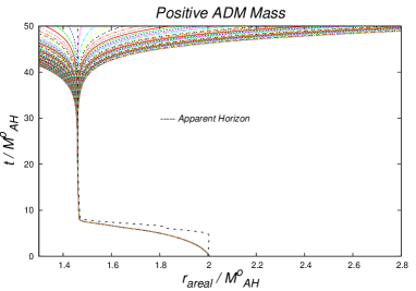
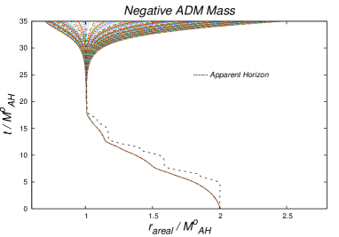
Figure 2: In the top panels we present the behavior of the different masses versus the coordinate time for the exponential potential and both, positive and negative ADM mass cases. The solid line represent the mass of the apparent horizon, the bold dashed line is the Misner-Sharp mass and the thin dashed line is the ADM mass of the space-time. In the positive ADM mass the apparent horizon of the black hole reduces up to 30 percent of its initial mass whereas in the negative case it is reduced up to 50 percent. In the bottom panel we show a set of outgoing null rays that help estimating approximately the location of the event horizon. For comparison we also show the location of the apparent horizon: at early stages of the accretion the apparent horizon lies outside of the event horizon, which is not surprising given that the energy conditions are not fulfilled and we notice that after the system has stabilized the event horizon and the apparent horizon coincide.

Figure 3: We show the convergence of the $L_{2}$ norm of the violation of the Hamiltonian, momentum and $G^{r}$ constraints to zero for positive and negative ADM mass cases.

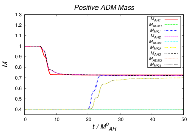
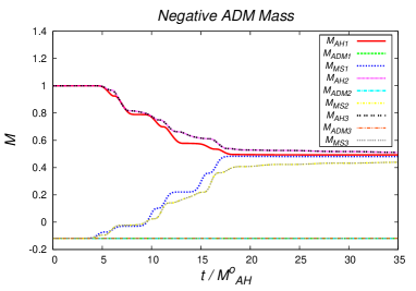
Figure 4: In these plots, we show the behavior of the apparent horizon, Misner-Sharp and ADM masses with three self-interaction potentials: i) curves with subindex 1 correspond to the exponential potential. ii) curves with subindex 2 correspond to the quadratic potential. iii) Curves with subindex 3 correspond to the quartic potential. In the case of the exponential potential the decrease is faster than in the other cases, however the final mass of the horizon is not quite different considering that the scalar field profile is so free that the in-going profile depends on the scalar field potential.

IV Conclusions

We present the full non-linear spherical accretion of a phantom scalar field with various potentials into a black hole.

This accretion process is very efficient at reducing the black hole horizon area, which is a potentially important process that may impose restrictions on the existing black hole masses, or for instance primordial black holes. In our simulations we were able to reduce the mass of the initial black hole up to 50$\%$. Attempts to reduce the area even further presents difficulties with our approach due to the steep gradients in the equations near the origin, and other techniques might be implemented in order to sort this problem out.

We show that the final mass of the black hole’s horizon is nearly independent of the potential used. This results is physically interesting because the process of area reduction will apply independently of the cosmologically motivated potential used.

We show that even though the Lagrangian (1) of the scalar field corresponds to a phantom field, at local scales the radial equation of state is always $p/\rho\geq-1$, and it depends on space and time, with values ranging from a cosmological constant equation of state $\omega=-1$ up to a stiff mater $\omega=1$.

We want to stress the importance of the equation of state of the scalar field given by the Lagrangian (1), and point out that perhaps the big rip scenario would strongly depend on the homogeneity and isotropy of the scalar field. We have shown how much the equation of state can depend on space and time for the model of a scalar field, at least in the strong gravitational field regime.

The astrophysical possibility of this accretion process strongly depends on the chance of having a phantom scalar field located near a black hole with a rather sharp profile.

References

- (1) P. S. Corasaniti et al., Foundations of observing dark energy dynamics with the Wilkinson Microwave Anisotropy Probe. Phys. Rev. D 70, 083006, 2004.
- (2) Babichev E., Dokuchaev V., and Eroshenko Yu.. Black hole mass decreasing due to phantom energy accretion. Phys. Rev. Lett., 93, 021102 (2004).
- (3) Gao Ch., Chen X., Faraoni V., and Shen Y-G, Does the mass of a black hole decrease due to the accretion of phantom energy? Phys. Rev. D 78, 024008 (2008).
- (4) González J.A., and Guzmán F.S., Accretion of phantom scalar field into a black hole. Phys. Rev. D 79, 121501 (2009).
- (5) Brown J.D., BSSN in spherical symmetry. Class. Quantum Grav., 25, 205004 (2008).
- (6) Thornburg J., A 3+1 computational scheme for dynamic spherically symmetric black hole space-times II: time evolution. Phys. Rev. D 59, 104007, (1999).
- (7) M. Shibata, T. Nakamura, Evolution of three dimensional gravitational waves: harmonic slicing case. Phys. Rev. D 52 5428, 1995. T. W. Baumgarte, S. L. Shapiro, On the numerical integration of Einstein’s field equations. Phys. Rev. D 59 024007,1999.
- (8) John G. Baker, et al.. Gravitational wave extraction from inspiraling configuration of merger black holes. Phys. Rev. Lett. 96, 111102 (2006).
- (9) M. Campanelli, et al., Accurate evolution of orbiting black hole binaries without excision. Phys. Rev. Lett. 96, 111101 (2006).
- (10) S. Brandt, B. Bruegmann, A simple construction of initial data for multiple black holes. Phys. Rev. Lett 78 3606, 1997.
- (11) Brown J.D., 2005, Conformal invariance and the conformal–traceless decomposition of the gravitational field. Phys. Rev. D 71, 104011.
- (12) Brown J. D. et al., Excision without excision: the relativistic turducken. Phys. Rev. D 76, 051503 (2007).