Abstract

In a nonlinear optical fiber communication (OFC) system with signal power much stronger than noise power, the noise field in the fiber can be described by linearized noise equation (LNE). In this case, the noise impact on the system performance can be evaluated by moment-generating function (MGF) method. Many published MGF calculations were based on the LNE using continuous wave (CW) approximation, where the modulated signal needs to be artificially simplified as an unmodulated signal. Results thus obtained should be treated carefully. More reliable results can be obtained by improving the CW-based LNE with the accurate LNE proposed by Holzl$\ddot{\mbox{o}}$hner et al in Ref. [1]. In this work we show that, for the case of linearized noise amplified by EDFAs, its MGF can be calculated by obtaining the noise propagation information directly from the accurate LNE. Our results agree well with the experimental data of multi-span DPSK systems.

OCIS codes: (060.2330) Fiber optics communications; (060.4370) Nonlinear optics,fiber; (060.5060) Phase modulation;(190.4410) Nonlinear optics, parametric process.

1 Introduction

The amplified spontaneous emission (ASE) noise from optical amplifiers, e.g., Erbium Doped Fiber Amplifiers (EDFAs), is one of the fundamental reasons for the bit-error-rate (BER) in an optical fiber communication (OFC) system. For an OFC system with non-negligible Kerr nonlinearity, the ASE impact evaluation is complicated due to the nonlinear interaction between signal and ASE noise. In the case of signal power much stronger than the noise power, the noise-noise beating is relatively small so that the noise field in the fiber can be approximately described by linearized noise equation (LNE), which was proposed separately in Ref. [1] and Refs. [2]-[8].

Noise propagator is a matrix used to show noise field propagation in the fiber. In the case of linear perturbation, it is independent of the specific noise realizations, which makes it possible to calculate the moment-generating function (MGF) of the filtered photoelectric current at the receiver [1]-[8].

MGF method is an approach making use of MGF to evaluate the noise impact on the system performance. Now, it is well known that this method is accurate for various linear OFC systems. For nonlinear OFC systems, the MGF method can also be applied, provided their noise fields obey LNE. One can see this from Doob’s theorem, which means that, in a linearizable system driven by Gaussian-distributed noise, each of the independent random variable keeps Gaussian (cf. P. 35 of Ref. [9]). Thus the MGF of the received photoelectric current can be calculated as those for linear OFC systems.

The common form of LNE [2]-[8] is based on the continuous wave (CW) assumption, i.e., the noise-free signal in the LNE is artificially simplified as a CW wave. As a result, a semi-analytical form of noise propagator and the noise power spectral density (PSD), so called parametric gain (PG), can be obtained. The drawback of this simplification is that the noise-free signal in this LNE neglects chromatic dispersion (CD) effect. As a result, the couplings between noise components (in frequency domain) cannot be taken into account.

A LNE beyond CW, named accurate LNE in this work, was first proposed and discussed in Ref. [1]. Dynamically taking into account the local CD and Kerr nonlinearity along the fiber, this LNE provides accurate noise information, with its computational cost being much higher than the CW approach. For example, given a noise-free signal obtained from nonlinear Schr$\ddot{\mbox{o}}$dinger equation (NLSE), the computation required to update the accurate LNE has cubic complexity in the number of Fourier components [1]. To reduce the computational complexity, covariance matrix method (CMM) was proposed in Ref. [1], where the noise covariance matrix was obtained by processing large noise realizations. In Refs. [10, 11], the computational cost of CMM was further reduced by a deterministic approach using perturbation solution. Since the raw covariance matrix obtained from NLSE via Monte Carlo noise realizations [1] or perturbation solution [10, 11] may contain nonlinear noise contribution, it needs to be separated from the nonlinearity-induced phase and timing jitter. Thus, the obtained pdfs of the receiver voltage agrees well with Monte Carlo simulation [1, 10, 12].

With the help of linear perturbation, the noise covariance matrix can also be solved from its ordinary differential equation (ODE) proposed by [1, 13]. The covariance matrix obtained by solving such linear ODE does not need jitter separation, although this ODE is more complicated than the accurate LNE [13]. So far there is little comparison between the approaches of Ref. [13] and Refs. [1, 10, 11].

In this work, we simplify the CMM by showing that the noise propagator matrix can be obtained directly from the accurate LNE. Therefore, there is no nonlinearity-induced jitter. To effectively reduce the computational complexity in updating the LNE, one can decompose the Kerr effect related matrix into a symmetric and an antisymmetric matrices [cf. the discussion after Eq. (35) in Appendix A]. Making use of the fourth-order Runge-Kutta in the interaction picture (RK4IP) method [14, 15], the accurate LNE can be solved with large step size, as detailed in Sec. 2. We evaluate the impacts of noise propagator on moment-generating function (MGF) and BER in Sec. 3. The accuracy of this new approach depends on how far the linearized noise deviates from the actual noise. To numerically verify this new approach, we consider the BERs in a 20-span DPSK system with nonlinear phase of $\bar{\Phi}_{N}=0.2\pi$ [5] in Sec. 5. Our BER calculations agree well with the published CMM results. In Sec. 5, we also simulate the experiments of the multi-span DPSK systems discussed in Ref. [7] and show that, to fit the experimental data, one needs to take into account the nonlinearity induced phase difference between noise and noise-free signal, which will affect the signal-noise beating significantly.

2 Noise propagator obtained from the accurate LNE

In an OFC system amplified by EDFAs, the noise propagator is a fundamental matrix that determines the noise impacts on MGF and BER. In this section, we show that the noise propagator matrix in a fiber of length $L$ can be obtained from the accurate LNE given by Eq. (37). For a multi-span OFC system, one needs to introduce an equivalent noise propagator which can be obtained from PG.

2.1 Noise propagator in a fiber of length $L$

The noise propagator in a fiber of length $L$ can be obtained by extending the RK4IP in Refs. [14, 15] to the accurate LNE given by Eq. (37) in Appendix A, where the linear operator $\hat{L}$ is associated with CD effect, whereas the nonlinear operator $\hat{N}$ is caused by Kerr nonlinearity. By introducing $\tilde{a}=e^{\hat{L}(z-z_{0})}\tilde{a}^{I}$ and $\hat{N}^{I}=e^{-\hat{L}(z-z_{0})}\hat{N}e^{\hat{L}(z-z_{0})}$, Eq. (37) in the interaction picture (IP) has the form

$$\frac{d\tilde{a}^{I}}{dz}=\hat{N}^{I}\tilde{a}^{I}$$ (1)

Taking $z_{0}=z_{n}+h/2$ with step size $h=z_{n+1}-z_{n}$ and denoting $\tilde{a}_{n}=\tilde{a}(z_{n})$, $\tilde{a}_{n+1}=\tilde{a}(z_{n+1})$, $\hat{N}^{I}_{n}=e^{\hat{N}h/2}\hat{N}(z_{n})e^{-\hat{N}h/2}$, $\hat{N}^{I}_{n+1/2}=\hat{N}(z_{n}+h/2)$, and $\hat{N}^{I}_{n+1}=e^{-\hat{L}h/2}\hat{N}(z_{n+1})e^{\hat{L}h/2}$, one can use RK4IP [14, 15] to to solve Eq. (1) with

$$\tilde{a}_{n+1}=e^{\hat{L}h/2}[\tilde{a}_{n}^{I}+\frac{hk_{1}}{6}+\frac{hk_{2}}{3}+\frac{hk_{3}}{3}+\frac{hk_{4}}{6}]$$

$$\tilde{a}_{n}^{I}=e^{\hat{L}h/2}\tilde{a}_{n}$$

$$k_{1}=\hat{N}_{n}^{I}\tilde{a}_{n}^{I}=e^{\hat{L}h/2}\hat{N}(z_{n})\tilde{a}_{n}\equiv\hat{k}_{1}\tilde{a}_{n}$$

$$k_{2}=\hat{N}^{I}_{n+1/2}[\tilde{a}_{n}^{I}+\frac{hk_{1}}{2}]=\hat{N}(z_{n}+h/2)[e^{\hat{L}h/2}+\frac{h\hat{k}_{1}}{2}]\tilde{a}_{n}\equiv\hat{k}_{2}\tilde{a}_{n}$$

$$k_{3}=\hat{N}^{I}_{n+1/2}[\tilde{a}_{n}^{I}+\frac{hk_{2}}{2}]=\hat{N}(z_{n}+h/2)[e^{\hat{L}h/2}+\frac{h\hat{k}_{2}}{2}]\tilde{a}_{n}\equiv\hat{k}_{3}\tilde{a}_{n}$$

$$k_{4}=\hat{N}_{n+1}^{I}[\tilde{a}_{n}^{I}+hk_{3}]=e^{-\hat{L}h/2}\hat{N}(z_{n+1})e^{\hat{L}h/2}[e^{\hat{L}h/2}+h\hat{k}_{3}]\tilde{a}_{n}\equiv\hat{k}_{4}\tilde{a}_{n}$$ (2)

or

$$\tilde{a}_{n+1}=\Bigg{(}e^{\hat{L}h/2}\bigg{[}e^{\hat{L}h/2}+\frac{h\hat{k}_{1}}{6}+\frac{h\hat{k}_{2}}{3}+\frac{h\hat{k}_{3}}{3}\bigg{]}+\frac{h}{6}\hat{N}(z_{n+1})e^{\hat{L}h/2}(e^{\hat{L}h/2}+h\hat{k}_{3})\Bigg{)}\tilde{a}_{n},$$ (3)

which means the noise propagator for the fiber of length $h=z_{n+1}-z_{n}$ can be calculated as

$$H(z_{n+1},z_{n})=e^{\hat{L}h/2}\bigg{[}e^{\hat{L}h/2}+\frac{1}{3}(\frac{h}{2}\hat{k}_{1}+\frac{2h}{2}\hat{k}_{2}+h\hat{k}_{3})\bigg{]}+\frac{h}{6}\hat{N}(z_{n+1})e^{\hat{L}h/2}\bigg{[}e^{\hat{L}h/2}+h\hat{k}_{3}\bigg{]}$$ (4)

For the fiber of length $L$, the noise propagator has the form

$$p_{n}(L,0)=H(L,L-h_{L})\cdots H(h_{1},0).$$ (5)

Note that the RK4IP used here is different from the RK4IP in Ref. [15], where what to be solved was the noise-free signal (a 1D matrix), while here what we want is the noise propagator (a 2D matrix). The computational complexity for this 2D matrix is $O(N_{w}^{3})$, due to that each $\hat{k}_{i}$ ($i=2,3,4$) in Eq. (2) needs one dense matrix multiplication. Here $N_{w}$ is the number of Fourier components used for signal representation, as mentioned between Eqs. (35) and (36).

2.2 Equivalent noise propagator of a multi-span system

As discussed in Appendix A, the ASE from an EDFA can be modeled as additive white Gaussian noise (AWGN) with its variance given by Eq. (38). Given the ASE injected at the input of a fiber and the noise propagator obtained from Eqs. (2), (4), and (5), the noise PSD (or PG) at the output of a fiber of length $L$ can be written as [1, 5, 7, 8]

$$PG_{1}=p_{n}(L,0)\sigma^{2}Ip_{n}^{T}(L,0)=\sigma^{2}p_{n}(L,0)p_{n}^{T}(L,0),$$ (6)

where $I$ is a unit matrix and Eq. (38) has been used. In Eq. (6), $p_{n}^{T}$ is the transpose of $p_{n}$.

For a $K$-span system consisting of $(K+1)$ EDFAs (cf. Fig. 4), its PG has the form

$$\widehat{PG}=\big{(}G\sigma_{in}^{2}+\sigma^{2}\big{)}P_{n}(K,0)P_{n}^{T}(K,0)+\sigma^{2}\sum_{k=1}^{K}P_{n}\big{(}K,k\big{)}P_{n}^{T}\big{(}K,k\big{)},$$

$$P_{n}\big{(}K,k\big{)}=p_{n}\Big{(}KL,(K-1)L\Big{)}\cdots p_{n}\Big{(}(k+1)L,kL\Big{)},\;\;\;\;\;(k=0,1,\cdots,K-1)$$

$$P_{n}\big{(}K,K\big{)}=I,$$ (7)

where $\sigma_{in}^{2}=N_{\mathrm{in}}/(2T_{0})$ and $\sigma^{2}$ is given by Eqs. (21) and (38). In Eq. (7), the real symmetric matrix $\widehat{PG}$ is positive definite. It can be factorized as

$$\widehat{PG}=\sigma^{2}P_{n,eq}P_{n,eq}^{T},$$ (8)

where the equivalent noise propagator $P_{n,eq}$ can be obtained either by using Cholesky decomposition or symmetric (square root) decomposition [16]. The latter yields $P_{n,eq}=P_{n,eq}^{T}$.

3 MGF calculation

With the noise propagator matrix, one can evaluate the BER in the OFC system by calculating the MGF of the electrically filtered current $I(t_{\mathrm{s}})$ expressed using Karhunen-Lo$\grave{\mbox{e}}$ve series expansion (KLSE).

Due to the noise in the OFC system, the received (or filtered photoelectric) current fluctuates around its expectation value. The MGF of such current is a useful form of its probability distribution. To get a simple form of MGF, the received current needs to be expressed using KLSE. For a nonlinear OFC system with its noise being linearizable, the KLSE form of the received current can be formulated as Eq. (49) and the related formulas in Appendix B. All the parameters for the nonlinear case are generalized from those for the linear case, which has been well discussed in Refs. [17, 18] and other publications. In Eqs. (48) and (49), the Dirac notation $|\tilde{Z}\rangle$ is used to represent the normalized noise (in Re-Im form) expressed by Karhunen-Lo$\grave{\mbox{e}}$ve bases (in Re-Im form). Averaging $|\tilde{Z}\rangle_{i}$ ($i=1,\cdots,4M_{n}+2$) with formula [17, 18]

$$E\Big{[}\exp\Big{(}s(\tilde{\lambda}c^{2}+2c\tilde{b})\Big{)}\Big{]}=\!\!\int_{-\infty}^{\infty}\!\!\frac{dc}{\sqrt{2\pi\sigma^{2}}}\exp(-\frac{c^{2}}{2\sigma^{2}})\exp[s(\tilde{\lambda}c^{2}+2c\tilde{b})]=\frac{\exp[\frac{2\sigma^{2}s^{2}\tilde{b}^{2}}{1-2\sigma^{2}s\tilde{\lambda}}]}{\sqrt{1-2\sigma^{2}s\tilde{\lambda}}},$$ (9)

the MGF of the filtered current, denoted as $\Psi_{t_{\mathrm{s}}}(s)$ here, can be written as

$$\Psi_{t_{\mathrm{s}}}(s)=E\Big{[}\exp[sI(t_{\mathrm{s}})]\Big{]}=\exp[sI_{\mathrm{ss}}(t_{\mathrm{s}})]\prod_{i=1}^{4M_{n}+2}\frac{\exp[\frac{2\sigma^{2}s^{2}\tilde{b}_{i}^{2}(t_{\mathrm{s}})}{1-s\beta_{i}}]}{(1-s\beta_{i})^{\xi}},\;\;\;\;(\beta_{i}=\!2\sigma^{2}\tilde{\lambda}_{i})$$ (10)

where $I(t_{\mathrm{s}})$ is the filtered photoelectric current at time $t_{\mathrm{s}}$. It consists of signal-signal beating ($y_{ss}$), noise-noise beating ($y_{nn}$), and signal-noise beating ($y_{ns}$), which are detailed in Eqs. (39) and (49) respectively. In Eq. (10), $\tilde{b}_{i}(t_{\mathrm{s}})$ is the $i$th component of $|\tilde{b}(t_{\mathrm{s}})\rangle$ in (49), while $\tilde{\lambda}_{i}$ is the power of $i$th component of the noise in Karhunen-Lo$\grave{\mbox{e}}$ve presentation. In Eq. (10), $\sigma^{2}$ is given by Eq. (38). In this work, we take $\xi=1/2$ for polarized noise.

With the help of Eq. (10) as well as Eqs. (7) and (8) in Ref. [18], the BER can be calculated.

4 OSNR at the receiver

For an optical system with ASE power being much larger than other noise sources, the OSNR with reference bandwidth $B_{r}$ (0.1nm) can be calculated as

$$OSNR_{0.1nm}=\frac{\bar{P_{s}}}{P_{ASE}(B_{r})}.$$ (11)

In Eq. (11), $\bar{P_{s}}$ is the time-averaged (noise free) signal power, while $P_{ASE}(B_{r})$ is the noise power within $B_{r}$. To obtain $\bar{P_{s}}$ and $P_{ASE}(B_{r})$, one needs to notice that the measurement bandwidth $B_{m}$ [e.g., the bandwidth of the transfer function of an optical spectrum analyzer (OSA)] may not be the same as $B_{r}$. Thus the $\bar{P_{s}}$ in Eq. (11) becomes the power of the signal filtered by $B_{m}$, while $P_{ASE}(B_{r})$ becomes the ASE filtered by $B_{m}$ and weighted by a factor $B_{r}/B_{m}$ [19].

In a linear optical system, the ASE noise along the fiber can be treated as AWGN. Thus, for the system of Fig. 4, its OSNR can be simply calculated as

$$OSNR_{L,0.1nm}=\frac{\bar{P_{s}}}{P_{ASE}(B_{m})}\times\frac{B_{m}}{B_{r}}\;\;\;\;\;\;\Big{(}P_{ASE}(B_{m})=[GN_{in}+N_{0}(K+1)]B_{m}\Big{)},$$ (12)

where $P_{ASE}(B_{m})$ is the ASE power within $B_{m}$ and $N_{0}$ is given by Eq. (21). In Eq.(12), the filter ($B_{m}$) effect on the ASE has been neglected.

In a nonlinear optical system, the ASE noise “amplified by” PG cannot be treated as a white noise. Similar to the noise-noise beating given in Eq. (49), the measured ASE power will only relate with the self-beating terms of the noise, which yields

$$OSNR_{NL,0.1nm}=\frac{\bar{P_{s}}}{P_{ASE}(B_{m})}\times\frac{B_{m}}{B_{r}}\;\;\;\Big{(}P_{ASE}(B_{m})=Tr(O^{T}_{m}\widehat{PG}O_{m})\sigma^{2}=Tr(\widehat{PG}O_{m}O^{T}_{m})\sigma^{2}\Big{)}.$$ (13)

Here $O_{m}$ is the low-pass transfer function of the bandpass filter (bandwidth $B_{m}$). In Eq. (13), $\sigma^{2}$ and $\widehat{PG}$ are given by Eq. (38) and Eq. (7), respectively.

In the case of traditional OSA-based out-of-band OSNR monitoring, the ASE power can be interpolated using

$$P_{ASE}(B_{m},\pm\Delta\lambda)=\frac{Tr\Big{[}\widehat{PG}\Big{(}O_{m}(-\Delta\lambda)O^{T}_{m}(-\Delta\lambda)+O_{m}(+\Delta\lambda)O^{T}_{m}(+\Delta\lambda)\Big{)}\Big{]}\sigma^{2}}{2},$$ (14)

where $O_{m}(\pm\Delta\lambda)$ is the filter function centered at $\pm\Delta\lambda$. When $\Delta\lambda=0$, Eq. (14) returns to the ASE power in Eq. (13), where $P_{ASE}(B_{m})\equiv P_{ASE}(B_{m},0)$.

Fig. 1: BER versus received OSNR for a 20Gb/s 20-span RZ-DPSK system with $\bar{\Phi}_{NL}=0.2\pi$. Solid: obtained using CMM of Ref. [1]. Dashed (dotted): improved CW approach of Ref. [5] with CW power being peak power (average power), respectively. Dash-dotted: RK4IP approach. All curves, except the dash-dotted, are obtained from Fig. 8 of Ref. [5].

5 Applications to DPSK systems

To show that the new approach to get the noise propagator is numerically applicable, we will compare our RK4IP results with the CMM results given by Ref. [5] and with the experimental data given by Ref. [7]. Both consider systems with $R_{b}=$20 Gb/s, using RZ-50$\%$ DPSK modulation. In the receiver, the optical filter is Gaussian type, while the electric filter is the fifth-order Bessel type. In the following calculations, we set $T_{0}=NT_{b}$ by changing $\mu$ in Eq. (41). This means, given the noise propagator matrix, the computational cost for BER is much higher than that in the linear case. For BER calculations, the length of the de Bruijn sequence is $N=2^{5}$ [17]. Based on the relation between the RK4IP step and the fiber dispersion length ($L_{D}$) or nonlinear length ($L_{N}$) discussed in Ref. [15] as well as the detailed fiber parameters in the following discussion, we let the RK4IP step for the transmission fiber ($h_{tr}$) and that for the DCF fiber ($h_{DCF}$) be related with $h_{tr}:h_{DCF}=(5\sim 6):1$. The value of $h_{tr}$ and the required computational time will be detailed below.

5.1 Comparison with CMM results

We consider the 20-span DPSK system discussed in Ref. [5], where BERs using the CMM and the (improved) CW approaches were plotted against the received OSNR in the Fig. 8 of Ref. [5]. In fact this system is basically the same as the one shown in Fig. 4 in Appendix A, provided that one removes the pre- and postcompensating fibers and their amplifiers in the Fig. 2 of Ref. [5] and removes the first EDFA and $N_{in}$ in our Fig. 4. Thus the first term of $\widehat{PG}$ [in Eq. (7)] needs to be ignored. Like Refs. [5, 20], where OSNR was calculated in the absence of PG, we obtain OSNR from Eq. (12) with $N_{in}=0$ and $(K+1)$ being replaced by $K$. According to Ref. [5], we change OSNR by changing the $n_{sp}$ in Eq. (21). As plotted in Fig. 4, each span contains a transmission fiber followed by a dispersion-compensating fiber (DCF). The transmission fiber is $l=$100 km long with its CD parameter $D_{tx}=8$ ps/nm/km. Each span is fully compensated. The nonlinear phase accumulated in the fiber, defined as $\bar{\Phi}_{NL}=\int_{0}^{z}\gamma(\xi)P_{in}e^{-\alpha(\xi)\xi}d\xi$ with $P_{in}$ being the time averaged signal power (at the input of the fiber), is $0.2\pi$. The bandwidth of the optical (electrical) filter in the receiver is $B_{o}=1.8R_{b}$ ($B_{e}=0.65R_{b}$), respectively.

To let our results be reproducible, we provide, as detailed as possible, other related parameters below. The DCF in each span is 8 km long with $D_{DCF}=-100$ ps/nm/km. Transmission fiber and DCF are assumed to have same fiber loss ($\alpha=$0.2 dB/km) and same nonlinear coefficient ( $\gamma=$2.0 /W/km). The EDFA in each span is used to compensate the total loss in the fiber of $L=(100+8)$ km. Therefore the signal power at the input of each span ($P_{in}$) keeps constant. Ignoring the nonlinear phase contribution of DCF [21], we set $P_{in}$=0.7307 mW, obtained from $\bar{\Phi}_{NL}=K\gamma P_{in}(1-e^{-\alpha l})/\alpha=0.2\pi$ with $K=20$ and $l=100$ km. The OSNR is obtained using Eq. (12) with $B_{m}/B_{r}=1.35$.

As shown in Fig. 1, the curve using the proposed RK4IP approach (dash-dotted) agrees very well with the CMM curve (solid) given by Ref. [5]. In Fig. 1, the curves using improved CW approach [5] with CW power being transmitted peak power (dashed) and average power (dotted) are plotted for comparison.

For each calculated point in Fig. 1, the CPU time for the noise propagator calculation is $\sim$1.8 hr with RK4IP step for transmission fiber ($20\times$100 km long) being $h_{tr}=$3.5 km. The CPU time for each BER calculation is $\sim$ 0.5 hr. In fact, $h_{tr}$ ranged within $0.3\sim 5$ km yields almost the same curve.

Fig. 2: BER versus received OSNR for the multi-span RZ-50$\%$ DPSK systems with $\bar{\Phi}_{NL}=0.9$. Each span consists of a SMF fiber (42 km long) and a DCF file (7 km long). Other fiber parameters were detailed in Table 1 of Ref. [7]. According to Fig. 7 (b) in Ref. [7], where the experimental curves for 5-, 10-, and 25-span systems were almost the same, here we replot these three curves using a thick solid curve.

Fig. 3: BER vs RX-OSNR for the 5-span RZ-50$\%$ DPSK system with $\bar{\Phi}_{NL}=0.9$. Other parameters are same as those used in Fig. 2. Solid: experimental results. Dotted (Dash-dotted): numerical calculation using RK4IP with (without) phase shift $\Delta$.

5.2 Comparison with experimental data

The optical system discussed in Ref. [7] can be modelled by Fig. 4, except that each EDFA should be replaced by an EDFA followed by an optical filter (Gaussian) $O_{lk}$ with bandwidth $B_{lk}=$5 nm. Also, the input noise $N_{in}$ needs to be filtered by an optical filter $O_{in}$ (Gaussian, $B_{in}=$3 nm). As a result, in Eq. (7), the noise propagator $p_{n}\Big{(}(k+1)L,kL\Big{)}$ ($k=0,\cdots,K-1$) should be replaced with $O_{lk}p_{n}\Big{(}(k+1)L,kL\Big{)}$, $P_{n}(K,K)=1$ with $P_{n}(K,K)=O_{lk}$, and $G\sigma^{2}_{in}P_{n}(K,0)P^{T}_{n}(K,0)$ with $G\sigma^{2}_{in}P_{n}(K,0)O_{in}O^{T}_{in}P^{T}_{n}(K,0)$. Since we only consider the curves plotted in Fig. 7 (b) of Ref. [7], each fiber ($L$ km long) in Fig. 4 contains a SMF (42 km long) followed by a DCF (7 km long). In our calculation, all the related fiber parameters are same as those given in Table 1 of Ref. [7]. In the receiver, the bandwidth of the optical filter is $1.87R_{b}$, while the bandwidth of the electrical filter is $0.75R_{b}$.

We first consider the back-to-back case. Similar to Ref. [7], we modify the 20Gb/s RZ-50$\%$ signal at the transmitter by comparing its calculated spectrum [22] and its measured spectrum[7]. Due to that the input noise $N_{in}$ is filtered by $O_{in}$, the OSNR is calculated using Eq. (13) with $B_{m}/B_{r}=0.95$, yielding the back-to-back RK4IP curve shown in Fig. 2.

For the 5-, 10-, 25-span systems, their accumulated nonlinear phases are calculated according to Eq. (48) of Ref. [7]. Because of the spectral modification of the input signal, the optical power at the input of each span $P_{in}=P_{SMF}$ is smaller than $E_{b}/T_{b}$, where $E_{b}$ is the energy per bit before the spectral modification. For example, to get nonlinear phase $\bar{\Phi}_{N}=0.9$ for the 25-span system, the fiber input power $P_{in}=P_{SMF}$ should be 1.516 mW, which means $E_{b}/T_{b}=$0.127 mW or $G(E_{b}/T_{b})=2.316$ mW ($G=18.197$). Different from the DPSK receiver shown in Fig.4, where the delay is $T_{b}=1/R_{b}=50$ ps, the delay in the receiver of Ref. [7] was $T^{\prime}_{b}$=(24.84 GHz)^-1=40.26 ps. Thus, the DPSK phase factors given in Eq. (40) should be modified as

$$D^{ss}_{l^{\prime}l}=\frac{e^{j\frac{2\pi l^{\prime}}{N^{\prime}}}\!+\!e^{-j\frac{2\pi l}{N^{\prime}}}}{2},\;\;D^{nn}_{m^{\prime}m}=\frac{e^{j\frac{2\pi m^{\prime}T^{\prime}_{b}}{T_{0}}}\!+\!e^{-j\frac{2\pi mT^{\prime}_{b}}{T_{0}}}}{2},\;D^{ns}_{ml}=\frac{e^{j\frac{2\pi mT^{\prime}_{b}}{T_{0}}-j\Delta}+e^{-j\frac{2\pi l}{N^{\prime}}+j\Delta}}{2},$$ (15)

with $N^{\prime}=N(T_{b}/T^{\prime}_{b})$, $T^{\prime}_{b}=T_{b}+\Delta T_{b}$. In Eq. (15), $\Delta$ is introduced as

$$\Delta=\phi_{0}-<\delta\phi>,$$ (16)

where $<\delta\phi>$, given by Eq. (52) in Appendix C, is the nonlinear phase difference between noise and noise-free signal. As shown in Fig. 2, all RK4IP curves ($\phi_{0}=0.31$) agree very well with the experiment results. The ASE power is calculated using Eq. (14) with $\Delta\lambda=2B_{m}$. In Eq. (16), $\phi_{0}$ is a calibration constant that basically shifts the RK4IP curves in the OSNR direction, while $<\delta\phi>$ determines the slope of the RK4IP curves. To show this, we plot in Fig. 3 the RK4IP results for the 25-span system with $\Delta=0.31-<\delta\phi>$ and $\Delta=0$. Also, we consider the RK4IP curves using Eq. (13) to calculate ASE power. Our results for the 5-span, 10-span, and 25-span systems confirm that there is almost no difference between the curve using Eq. (14) with $\phi_{0}=0.31$ and the curve using Eq. (13) with $\phi_{0}=0.57$.

In Eq. (16), the calibration constant $\phi_{0}$ can be temporally considered as a fitting parameter. As mentioned above, it basically affects the BER vs OSNR curve in the OSNR direction and is related with the detailed OSNR monitoring technique used in Ref. [7]. As there is few information about its OSNR measurement, evaluation of $\phi_{0}$ is expected to be discussed elsewhere.

In the above calculation, our CPU time for the noise propagator calculation is $\sim$0.8 hr with RK4IP step for transmission fibers ($25\times$40 km long) being $h_{tr}=$6.0 km. The CPU time for each BER calculation is $\sim$ 0.5 hr. The step size $h_{tr}$ within $0.3\sim 10$ km will result in almost the same curve.

6 Summary

For linear OFC systems, MGF method is useful for one to evaluate the noise impacts on BERs. This is true not only because it is computationally efficient for the cases with low BER (e.g., $<10^{-9}$) but also it can provide reliable information for the cases using coherent detection, which is now widely used in modern OFC systems. It is now well recognized that traditional Gaussian fitting Q-factor approximation is accurate for OOK detection, while MGF method is accurate for various linear OFC systems.

To extend the MGF method to a nonlinear OFC system, one needs to make sure its noise propagator varies within linear regime. This means the noise-noise interaction needs to be neglected and the noise field should follow LNE.

In CMM of Refs. [1, 11, 12], the noise propagator was obtained from NLSE. It may contain the nonlinearity-induced jitter, which is beyond the linear regime and should be removed. In this work we simplify the CMM by directly solving the accurate LNE [Eq. (1)] with RK4IP. Like the CW approximations (cf. Refs. [2]-[8] and many others) as well as the approach of Ref. [13], where the noise propagation information obtained from the related linearized noise equation is automatically free from nonlinearity-induced jitter, the noise propagator obtained from accurate LNE also varies within linear regime.

To numerically verify this new approach, we consider a 20-span RZ-DPSK system discussed in Ref. [5]. The BERs obtained using this new RK4IP agree well with those using CMM in Ref. [5]. Taking account the phase difference between noise and noise-free signal leads to quantitative matching between numerical evaluation and experimental result [7].

Appendix A: Accurate LNE in the EDFA-based systems

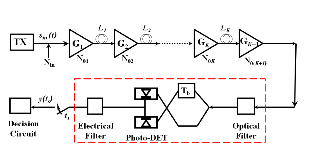
Fig. 4: Low-pass equivalent optical model. The receiver consists of optical and electrical filters and DPSK balance detection. Our calculations, except those in Sec. 5.1, are based on the assumptions that $N_{0k}=N_{0}$ and $G_{k}=G$ [$k=1,2,...(K+1)$]. Also, the fiber in each span is assumed to have same length ($L$ km) and same loss ($\alpha$ dB/km). $\mathrm{N}_{\mathrm{in}}$ is the ASE noise added at the transmitter. Changing $\mathrm{N}_{\mathrm{in}}$ will change the OSNR at the receiver. In a typical balanced DPSK receiver, the delay in one branch of the interferometer is $T_{b}=1/R_{b}$. In this work, $R_{b}=20$ Gb/s.

The optical field $u(z,t)$ in a fiber satisfies

$$\frac{\partial u}{\partial z}=j\frac{\beta_{\omega\omega}}{2}\frac{\partial^{2}u}{\partial t^{2}}+\frac{\beta_{\omega\omega\omega}}{6}\frac{\partial^{3}u}{\partial t^{3}}-j\gamma|u|^{2}u-\frac{\alpha}{2}u,$$ (17)

where $\alpha$ is the fiber loss and $\beta_{\omega\omega}=\partial^{2}\beta/\partial\omega^{2}$ relates to the CD parameter $D(\lambda)$ (ps/nm/km) with $\beta_{\omega\omega}$=-$\frac{\lambda^{2}D(\lambda)}{2\pi c}$ (c=3$\times$10⁸ m/s). The slope parameter $\beta_{\omega\omega\omega}=(\frac{\lambda}{2\pi c})^{2}[2\lambda D(\lambda)+\lambda^{2}D^{\prime}(\lambda)]$ [$D^{\prime}(\lambda)=\frac{dD(\lambda)}{d\lambda}$ (ps/nm${}^{2}\cdot$km)] can be neglected if bit rate $R_{b}$ satisfies $R_{b}>|\beta_{\omega\omega}/\beta_{\omega\omega\omega}|$ [17].

Introducing the transformation $u(z,t)=v(z,t)e^{-\alpha z/2}$, Eq. (17) can be reduced as

$$\frac{\partial v}{\partial z}=j\frac{\beta_{\omega\omega}}{2}\frac{\partial^{2}v}{\partial t^{2}}+\frac{\beta_{\omega\omega\omega}}{6}\frac{\partial^{3}v}{\partial t^{3}}-je^{-\alpha z}\gamma|v|^{2}v.$$ (18)

In a $K$-span system amplified by $(K+1)$ EDFAs (cf. Fig. 4), Eq. (18) can be modified as

$$\frac{\partial v}{\partial z}=j\frac{\beta_{\omega\omega}}{2}\frac{\partial^{2}v}{\partial t^{2}}+\frac{\beta_{\omega\omega\omega}}{6}\frac{\partial^{3}v}{\partial t^{3}}-je^{-\alpha z}\gamma|v|^{2}v-jw(z,t),$$ (19)

where $w(z,t)$ is the ASE forcing modeled as the complex AWGN with correlation

$$r(z,z^{\prime},t,t^{\prime})=E\{w(z,t)w^{*}(z^{\prime},t^{\prime})\}=\delta(t-t^{\prime})\delta(z-z^{\prime})\sum_{k=1}^{K+1}N_{0k}\delta(z-(k-1)L).$$ (20)

In Eq. (20), the fiber length in each span is assumed to be $L$ (km) long, According to Wiener-Kinchine theorem [23], $N_{0k}$ in Eq. (20) is the ASE PSD (in one polarization direction) at the output of the $k$th EDFA. Suppose each EDFA has the same gain $G$ and spontaneous-emission parameter $n_{sp}$, we have [17]

$$N_{0k}=N_{0}=n_{sp}(G-1)\hbar\omega\;\;\;\;\;\;\Big{(}k=1,2,...K,(K+1)\Big{)}$$ (21)

Decomposing optical field $v(z,t)$ in the fiber into noise-free field $v_{0}(z,t)$ and its perturbation $\delta v(z,t)$ [i.e., $v(z,t)=v_{0}(z,t)+\delta v(z,t)$] and assuming that $|v_{0}|>>|\delta v|$ (so that the nonlinear terms of $\delta v$ can be neglected), Eq. (19) can be decomposed as [1]

$$\frac{\partial v_{0}}{\partial z}=j\frac{\beta_{\omega\omega}}{2}\frac{\partial^{2}v_{0}}{\partial t^{2}}+\frac{\beta_{\omega\omega\omega}}{6}\frac{\partial^{3}v_{0}}{\partial t^{3}}-je^{-\alpha z}\gamma|v_{0}|^{2}v_{0}$$ (22)

$$\frac{\partial\delta v}{\partial z}=j\frac{\beta_{\omega\omega}}{2}\frac{\partial^{2}\delta v}{\partial t^{2}}+\frac{\beta_{\omega\omega\omega}}{6}\frac{\partial^{3}\delta v}{\partial t^{3}}-j2e^{-\alpha z}\gamma|v_{0}|^{2}\delta v-je^{-\alpha z}\gamma v_{0}^{2}\delta v^{*}-jw(z,t).$$ (23)

Noise equation Eq. (23) differs from common equations in that the real and imaginary parts of the complex noise field need to be treated separately [1].

Denoting $a_{l}=a(\omega_{l})=\int\delta ve^{-j\omega_{l}t}dt$ and the circulant matrices $[M_{\nu}]_{lm}=\nu_{l-m}$, $[M_{\mu}]_{lm}=\mu_{l+m}$ with

$$\nu_{l}=\nu(\omega_{l})=e^{-\alpha z}\int|v_{0}|^{2}e^{-j\omega_{l}t}dt,\;\;\;\;\mu_{l}=\mu(\omega_{l})=e^{-\alpha z}\int v_{0}^{2}e^{-j\omega_{l}t}dt,$$ (24)

in frequency domain, Eq. (23) has the form

$$\frac{da_{l}}{dz}=-j\frac{\beta_{\omega\omega}}{2}\omega_{l}^{2}a_{l}-j\frac{\beta_{\omega\omega\omega}}{6}\omega_{l}^{3}a_{l}-j2\gamma(z)[M_{\nu}]_{lm}a_{m}-j\gamma(z)[M_{\mu}]_{lm}a_{m}^{*}-jW_{l},$$ (25)

where $W_{l}=W(z,\omega_{l})$ is the Fourier component of the forcing term $w(z,t)$ in Eq. (19). As indicated in Ref. [1], since $|v_{0}|^{2}$ in (24) is real, $\nu_{l}=\nu_{-l}^{*}$. So $M_{\nu}$ in (25) is Hermitian, or, its real part $M_{\nu}^{R}$ is symmetric, while its imaginary part $M_{\nu}^{I}$ is anti-symmetric. Also, as $[M_{\mu}]_{km}=\mu_{k+m}$, both the real ($M_{\mu}^{R}$) and imaginary parts ($M_{\mu}^{I}$) of $M_{\mu}$ are symmetric.

The matrix form of Eq. (25) is

$$\frac{da}{dz}=\bar{L}a+\nu a+\mu a^{*}-jW$$ (26)

$$\bar{L}=jL_{CD},\;\;\;\nu=-2j\gamma(z)(M_{\nu}^{R}+jM_{\nu}^{I}),\;\;\mu=-j\gamma(z)(M_{\mu}^{R}+jM_{\mu}^{I})$$ (27)

Introducing $\tilde{a}=(a_{R},a_{I})^{T}$ (for $a=a_{R}+ja_{I}$) and $\tilde{W}=(W_{I},-W_{R})^{T}$ (for $-jW=W_{I}-jW_{R}$), Eq. (26) is equivalent to

$$\!\!\!\frac{d\tilde{a}}{dz}=(\hat{L}+\hat{\nu}+\hat{\mu})\tilde{a}+\tilde{W}$$ (28)

$$\!\!\!\hat{L}=\left(\begin{array}[]{cc}0&-L_{CD}\\ L_{CD}&0\end{array}\right),\;\;\hat{\nu}=\left(\begin{array}[]{cc}\nu_{AA}&-\nu_{SS}\\ \nu_{SS}&\nu_{AA}\end{array}\right),\;\;\hat{\mu}=\left(\begin{array}[]{cc}\mu_{R}&\mu_{I}\\ \mu_{I}&-\mu_{R}\end{array}\right),$$ (35)

with $(L_{CD})_{ij}=-[\frac{\beta_{\omega\omega}}{2}\omega^{2}+\frac{\beta_{\omega\omega\omega}}{6}\omega^{3}]\delta_{ij}$, $\nu_{AA}=2\gamma M_{\nu}^{I}$, $\nu_{SS}=-2\gamma M_{\nu}^{R}$, $\mu_{R}=\gamma M_{\mu}^{I}$, and $\mu_{I}=-\gamma M_{\mu}^{R}$. According to the discussion given below Eq. (25), $\hat{\nu}$ ($\hat{\mu}$) in Eq. (35) is antisymmetric (symmetric), respectively. Calculation of the Kerr term $(\hat{\nu}+\hat{\mu})$ according to Eq. (35) has the computational complexity much less than $O(N_{W}^{3})$, where $N_{W}$ is the number of Fourier components used for signal representation. In fact, the computational cost of this way is basically determined by the FFTs in Eq. (24), which has the computational complexity of $O(N_{W}logN_{W})$.

In frequency domain, ASE correlation relation (20) has its matrix form ( $\tilde{W}(\omega_{l})\rightarrow\tilde{W}_{l}\sqrt{\Delta f}$ )

$$E\{\tilde{W}_{l}(z)\tilde{W}_{l^{\prime}}^{*}(z^{\prime})\}=\delta_{z,z^{\prime}}\delta_{l,l^{\prime}}\sum_{k=0}^{K}\frac{N_{0}}{2T_{0}}\delta_{z,kL}\;\;\;\;(l=1,\cdots,4M_{n}+2),$$ (36)

where Eq. (21) has been used. In Eq. (36), $T_{0}=1/\Delta f$ and $M_{n}$ are given by Eq. (41). Eq. (36) means that Eq. (28) can be equivalently replaced by

$$\frac{d\tilde{a}}{dz}=(\hat{L}+\hat{N})\tilde{a};\;\;\;\;(\hat{N}=\hat{\nu}+\hat{\mu})$$ (37)

with boundary condition [25]

$$E\{\tilde{W}(z_{f})\tilde{W}^{*}(z_{f})\}=\frac{N_{0}}{2T_{0}}I\equiv\sigma^{2}I$$ (38)

with $I$ being a $(4M_{n}+2)\times(4M_{n}+2)$ unit matrix and $\sigma^{2}$ being the variance of the real or imaginary part of input ASE.

Appendix B: Filtered photoelectric current expressed using KLSE Given a linear optical system, based on the discussions in Ref. [17] and the notations introduced in Ref. [18], the filtered photoelectric current $I(t)$ can be expressed in the form of $I(t)=[\langle s^{o}(t+T_{b})+n^{o}(t+T_{b})|s^{o}(t)+n^{o}(t)\rangle+c.c.]/2$. Here $s^{o}(t)$ ($n^{o}(t)$) represents the signal (noise) field at the input of the optical filter. Dirac bra $\langle x|$ is the conjugate transpose (or Hermitian transpose) of Dirac ket $|x\rangle$ [$x=s^{o}(t),n^{o}(t),s^{o}(t)+n^{o}(t),etc.$]. The Dirac ket differs from usual complex vector in that the $i$th element of the latter is just the $i$th Fourier coefficient of the (signal or noise) field, while the $i$th element of the former is the product of the $i$th Fourier coefficient and its base function (cf. Eq. (17) in Ref. [18]). According to Refs. [17, 18], the filtered current in a linear system can be formally expressed as $I(t)=y_{ss}+y_{nn}+y_{ns}$ with ($l=-L_{s},\cdots L_{s}$; $m=-M_{n}\cdots M_{n}$)

$$y_{ss}(t_{\mathrm{s}})\!\!\! \!\!\!=\!\!\! \!\!\![\langle s^{o}(t_{\mathrm{s}}+T_{b})|R_{ss}|s^{o}(t_{\mathrm{s}})\rangle+c.c.]/2=\langle s^{o}(t_{\mathrm{s}})|R_{ss}^{D}|s^{o}(t_{\mathrm{s}})\rangle$$

$$y_{nn}(t_{\mathrm{s}})\!\!\! \!\!\!=\!\!\! \!\!\![\langle n^{o}(t_{\mathrm{s}}+T_{b})|R_{nn}|n^{o}(t_{\mathrm{s}})\rangle+c.c.]/2=\langle N^{o}|R_{nn}^{D}|N^{o}\rangle=\langle Z|\Lambda|Z\rangle$$

$$y_{ns}(t_{\mathrm{s}})\!\!\! \!\!\!=\!\!\! \!\!\![\langle n^{o}(t_{\mathrm{s}}+T_{b})|R_{ns}|s^{o}(t_{\mathrm{s}})\rangle+\langle n^{o}(t_{\mathrm{s}})|R_{ns}|s^{o}(t_{\mathrm{s}}+T_{b})\rangle+c.c.]/2$$ (39)

$$\!\!\!=\!\!\! \!\!\![\langle N_{in}|O^{\dagger}_{nn}R_{ns}^{D}|s^{o}(t_{\mathrm{s}})\rangle+c.c]=[\langle Z|b^{D}(t_{\mathrm{s}})\rangle+c.c.]$$

where $\Lambda\equiv U^{\dagger}O^{\dagger}_{nn}R_{nn}^{D}O_{nn}U=diag\{\lambda_{1},\cdots,\lambda_{2M_{n}+1}\}$, $|b^{D}(t_{\mathrm{s}})\rangle=U^{\dagger}O^{\dagger}_{nn}R_{ns}^{D}|s^{o}(t_{\mathrm{s}})\rangle$, and

$$\!\!\!\!\!(R_{ss}^{D})_{l^{\prime}l}=(R_{ss})_{l^{\prime}l}D^{ss}_{l^{\prime}l},\;\;(R_{nn}^{D})_{m^{\prime}m}\!=\!(R_{nn})_{m^{\prime}m}D^{nn}_{m^{\prime}m},\;\;(R_{ns}^{D})_{ml}=(R_{ns})_{ml}D^{ns}_{ml}$$

$$\!\!\!\!\!D^{ss}_{l^{\prime}l}=\frac{e^{j\frac{2\pi l^{\prime}}{N}}\!+\!e^{-j\frac{2\pi l}{N}}}{2},\;\;D^{nn}_{m^{\prime}m}=\frac{e^{j\frac{2\pi m^{\prime}T_{b}}{T_{0}}}\!+\!e^{-j\frac{2\pi mT_{b}}{T_{0}}}}{2},\;D^{ns}_{ml}=\frac{e^{j\frac{2\pi mT_{b}}{T_{0}}}+e^{-j\frac{2\pi l}{N}}}{2}.$$ (40)

In Eqs. (39)-(40), $|Z\rangle$ represents the decoupled Gaussian random variables with zero mean and real part and imaginary part variance of $\sigma^{2}$. The effects of the optical and electrical filters in the receiver are represented by matrices with their elements being $(O_{nn})_{mm^{\prime}}=\delta_{m,m^{\prime}}H_{o}(\frac{m}{T_{0}})$, $(O_{ss})_{ll^{\prime}}=\delta_{l,l^{\prime}}H_{o}(\frac{l}{NT_{b}})$ and $(R_{ss})_{ll^{\prime}}=H_{r}(\frac{l^{\prime}-l}{NT_{b}}),(R_{nn})_{mm^{\prime}}=H_{r}(\frac{m^{\prime}-m}{T_{0}}),(R_{ns})_{ml}=H_{r}(\frac{l}{NT_{b}}-\frac{m}{T_{0}})$. Due to the optical and electrical filters, signal (noise) components outside $\pm L_{s}$ ($\pm M_{n}$) can be neglected. Here [17]

$$L_{s}=\eta NT_{b}B_{o},\;\;M_{n}=\eta B_{o}T_{0},\;\;T_{0}=\mu(\frac{1}{B_{o}}+\frac{1}{B_{r}})\;.$$ (41)

For a nonlinear optical system, to get the noise propagator from the accurate LNE (28), one needs to separate complex numbers into their real and imaginary parts. Denoting the Re-Im form of a complex matrix $x$ as $\tilde{x}=\left(\begin{array}[]{cc}Re\{x\}&-Im\{x\}\\ Im\{x\}&Re\{x\}\end{array}\right)$ [where $x$ can be any complex matrix in Eq. (39)] and introducing $|n^{o}\rangle=P_{n,eq}|a_{0}\rangle$ with $|a_{0}\rangle$ being the AWGN from EDFA,

$$|\tilde{s}^{o}\rangle=\left[\begin{array}[]{c}Re\{|s^{o}\rangle\}\\ Im\{|s^{o}\rangle\}\end{array}\right],\;\;|\tilde{a}_{0}\rangle=\left[\begin{array}[]{c}Re\{|a_{0}\rangle\}\\ Im\{|a_{0}\rangle\}\end{array}\right],\;\;|\tilde{Z}\rangle=\left[\begin{array}[]{c}Re\{|Z\rangle\}\\ Im\{|Z\rangle\}\end{array}\right],$$ (48)

it is easy to generalize the noise related currents in Eq. (39) as [1, 5, 7, 8, 17]

$$\!\!\!\!\!\!\!\!y_{nn}(t_{\mathrm{s}})\!\!=\!\!\langle\tilde{a}_{0}|\tilde{U}\tilde{\Lambda}\tilde{U}^{T}|\tilde{a}_{0}\rangle\!\!\equiv\!\!\langle\tilde{Z}|\tilde{\Lambda}|\tilde{Z}\rangle\;\;\;\;\;(\tilde{\Lambda}\!\!=\!\!\tilde{U}^{T}P_{n,eq}^{T}\tilde{O}_{nn}^{T}\tilde{R}^{D}_{nn}\tilde{O}_{nn}P_{n,eq}\tilde{U}\!\!=\!\!diag\{\tilde{\lambda}_{1},\cdots,\tilde{\lambda}_{4M_{n}+2}\})$$

$$\!\!\!\!\!\!\!\!y_{ns}(t_{\mathrm{s}})\!\!=\!\!\langle\tilde{Z}|\tilde{U}^{T}P_{n,eq}^{T}\tilde{O}_{nn}^{T}\tilde{R}^{D}_{ns}\tilde{O}_{ss}|\tilde{s}^{o}(t_{\mathrm{s}})\rangle\!\!=\!\!\langle\tilde{Z}|\tilde{B}|\tilde{s}^{o}(t_{\mathrm{s}})\rangle\equiv\langle\tilde{Z}|\tilde{b}(t_{\mathrm{s}})\rangle\;\;\;(\tilde{B}\!\!=\!\!\tilde{U}^{T}P_{n,eq}^{T}\tilde{O}_{nn}^{T}\tilde{R}^{D}_{ns}\tilde{O}_{ss}),$$ (49)

where $P_{n,eq}$ can be obtained from Eqs. (2)-(5) and (7)-(8).

Appendix C: Nonlinearity induced phase difference between noise and noise-free signal I: The phase difference caused by $\mathrm{N_{in}}$

In this part, we assume that, in Fig. 4, the external noise injected at the transmitter ( $\mathrm{N_{in}}$ ) is much larger than the ASE noise from the EDFAs, which is true for the experiments discussed in Ref. [7]. Thus, one can only consider the phase difference caused by $\mathrm{N_{in}}$ and ignores the effect of $\mathrm{N}_{0k}$ ($k=1,\cdots,K$).

It is well known that, for the noise-free signal with its path average power being $\bar{P}$, its nonlinear phase accumulated at the fiber output is $\bar{\Phi}_{NL}=\bar{P}\gamma KL$, where $L$ is the fiber length of each span, as denoted in Fig. 4. Due to the optical power fluctuation $\delta\bar{P}$, the actual nonlinear phase becomes

$$\phi_{NL}=(\bar{P}+\delta\bar{P})\gamma KL.$$ (50)

Relative to the noise-free signal, the noise-induced phase change, $\phi_{NL}-\bar{\Phi}_{NL}$, varies randomly. The average variance of such phase noise can be calculated as

$$<\delta\phi^{2}>=\equiv<\phi_{NL}^{2}-\bar{\Phi}_{NL}^{2}>\approx 2\bar{P}<\delta\bar{P}>(\gamma KL)^{2}.$$ (51)

With the approximation of negligible $N_{0k}$ ($k=1\cdots K$), $<\delta\bar{P}>$ in Eq. (51) is basically caused by $\mathrm{N_{in}}$ in Fig. 4. For the experiments in Ref. [7], $\mathrm{N_{in}}$ is filtered with bandwidth of $B_{in}$=3nm. Thus, we have $<\delta\bar{P}>=G\mathrm{N_{in}}B_{in}$. Eq. (51) yields

$$<\delta\phi>\approx\sqrt{2}\bar{P}\gamma KL/\sqrt{\bar{P}/<\delta\bar{P}>}=\sqrt{2}\bar{\Phi}_{NL}/\sqrt{OSNR},$$ (52)

where $OSNR\approx\bar{P}/(G\mathrm{N_{in}}B_{in})$ is the input OSNR.

Considering that $\delta\bar{P}\geq 0$, we have $\phi_{NL}>\bar{\Phi}_{NL}$. This means $\phi_{NL}$ rotates faster than $\bar{\Phi}_{NL}$ and there is a phase difference between the actual optical field and the noise-free field. As part of the actual field, the noise field also has the same phase shift relative to the noise-free signal. Note that this phase shift will not affect signal-signal and noise-noise beatings. But it will affect the signal-noise beating. In fact, when calculating the signal-noise beating, the noise and signal should be treated consistently. Or, they should be considered within the same coordinate system. In this work, $<\delta\phi>$ given by Eq. (52) is approximated as the average of such phase shift. Our numerical results plotted in Figs. 2 and 3 confirm this approximation.

For the experiments in Ref. [7], we have $\bar{\Phi}_{NL}=0.9$. In this case, Eq. (52) yields

$$<\delta\phi>\approx 1/\sqrt{OSNR}\approx\pi/2-\mathrm{arctan}(\sqrt{OSNR}),$$ (53)

where $\mathrm{arctan}(x)+\mathrm{arctan}(1/x)=\pi/2$ and $\mathrm{arctan}(x)\approx x$ (for $x\rightarrow 0$) have been used. Obviously, $<\delta\phi>$ in Eq. (53) relates $\phi_{GM}$ in Eq.(23) of Ref. [26] with $<\delta\phi>+\phi_{GM}=\pi/2$. Also, $\phi_{0}$ in Ref. [26] now becomes $\phi_{0}+\pi/2\rightarrow\phi_{0}$ in Eq. (16), while $\Delta_{GM}$ in Ref. [26] is named as $\Delta$ in this work.

II: The phase difference caused by $\mathrm{N_{in}}$ and $\mathrm{N}_{0k}$ ($k=1,\cdots,K$)

For the $K$-span system of Fig. 4 with $N_{in}\neq 0$ and $K$ not being large enough and with the ASE from each EDFA being filtered by $O_{lk}$ and the ASE injected at the transmitter being filtered by $O_{in}$, Eq. (51) can be generalized as

$$<\delta\phi^{2}>=2\Big{[}GN_{in}B_{in}+N_{0}B_{lk}\frac{K}{3}(1+\frac{1}{K})(1+\frac{1}{2K})\Big{]}\bar{\Phi}_{NL}^{2}/\bar{P},$$ (54)

where $\sum_{k=1}^{K}k^{2}=\frac{K^{3}}{3}(1+\frac{1}{K})(1+\frac{1}{2K})$ has been used. Obviously, in the case of $GN_{in}B_{in}>>KN_{0}B_{lk}$ [7], Eq. (54) yields Eq. (52).

Acknowledgment

The authors acknowledge the financial support from Canada Research Chair program. The first author sincerely thanks Paolo Serena and Leonardo D. Coelho for providing their detailed calculations in Refs. [5, 7]. The authors wish to thank the anonymous reviewers for their valuable comments and suggestions.