A finite element exterior calculus framework for the rotating shallow-water equations

Abstract

We describe discretisations of the shallow water equations on the sphere using the framework of finite element exterior calculus, which are extensions of the mimetic finite difference framework presented in Ringler, Thuburn, Klemp, and Skamarock (Journal of Computational Physics, 2010). The exterior calculus notation provides a guide to which finite element spaces should be used for which physical variables, and unifies a number of desirable properties. We present two formulations: a “primal” formulation in which the finite element spaces are defined on a single mesh, and a “primal-dual” formulation in which finite element spaces on a dual mesh are also used. Both formulations have velocity and layer depth as prognostic variables, but the exterior calculus framework leads to a conserved diagnostic potential vorticity. In both formulations we show how to construct discretisations that have mass-consistent (constant potential vorticity stays constant), stable and oscillation-free potential vorticity advection.

1 Introduction

In a recent paper on horizontal grids for global weather and climate models, [1] listed a number of desirable properties that a numerical discretisation should have, which can be paraphrased as accurate representation of geostrophic adjustment, mass conservation, curl-free pressure gradient, energy conserving pressure terms, energy conserving Coriolis term, steady geostrophic modes, and absence/control of spurious modes. Of this list as presented here, the first property could be said to relate to the stability and accuracy of the discrete Laplacian formed from divergence and gradient operators, whilst the next five all relate to mimetic properties (i.e. the numerical discretisations exactly represent differential calculus identities such as $\nabla\times\nabla=0$), and the last property relates to the kernels of the various discretised operators (see [2, 3, 4] and related papers by Le Roux and coworkers for extended discussion of these issues in the context of finite element methods). In the context of the rotating shallow-water equations on the sphere, which represent the standard nonlinear framework for investigating horizontal grids for global models, the C-grid staggering on the latitude-longitude grid combined with an appropriate choice of reconstruction of the Coriolis term provides all of these properties, but leaves us with a grid system with a polar singularity. This, together with a need for models with variable resolution, has started a quest for alternative grids and discretisations that satisfy these properties.

The extension of the C-grid to triangular meshes (and the finite element analogue, the RT0-P0 discretisation) satisfies the first six properties and has been popular in both atmosphere and ocean applications ([5, 6]), however it is now well understood that the triangular C-grid supports spurious inertia-gravity mode branches because of the decreased ratio of velocity degrees of freedom (DOFs) to pressure DOFs relative to quadrilaterals (from 2:1 to 3:2) [7, 8]. More recently, a Coriolis reconstruction for the hexagonal C-grid was derived in [9] that provides the mimetic properties described above, and this was extended to arbitrary orthogonal C-grids (grids in which dual grid edges that join pressure points intersect the primal grid edges orthogonally) in [10]. The hexagonal C-grid has an increased ratio of velocity DOFs to pressure DOFs (from 2:1 to 3:1), and so does not support spurious inertia-gravity mode branches, but does have a branch of spurious Rossby modes. This reconstruction can be used to construct energy and enstrophy conserving C-grid discretisations for the nonlinear rotating shallow-water equations using the vector invariant form [11], in which mimetic properties are used to produce a velocity-pressure formulation in which the diagnosed potential vorticity is locally conserved in a shape-preserving advection scheme, and is consistent with the discrete mass conservation (i.e. constant potential vorticity stays constant in the unforced case).

Two directions remain outstanding from this approach, namely the relaxation of the orthogonality requirement which constrains cubed sphere grids so that grid resolution increases much more quickly in the corners than at the middle of the faces [12], and the construction of higher-order operators to avoid grid imprinting. Two recent papers by the authors attempted to address these issues. In [13] a framework was set up to generalise the mimetic approach of [11] to non-orthogonal grids, but the method of constructing sufficiently high-order operators was not clear. Meanwhile, in [14], it was shown that mixed finite element methods in the framework of finite element exterior calculus (see [15] for a review) provide the first six properties listed above, plus sufficient flexibility to adjust the ratio of velocity DOFs to pressure DOFs to 2:1 to avoid spurious mode branches. The BDFM1 space on triangles and the RTk hierarchy of spaces on quadrilaterals were advocated as examples of spaces that satisfy that ratio. However, in that paper it was not clear how the extension to nonlinear shallow-water equations would be made. In this paper we address both of these open questions by describing a finite element exterior calculus framework for the shallow-water equations, which enables us to write the equations in a very compact form that is coordinate-free, and reveals the underlying structure behind the mimetic properties. The goal is to have a numerical discretisation for the shallow water equations with velocity and layer thickness as prognostic variables, but with a conserved diagnostic potential vorticity. We shall discuss two formulations: a primal grid formulation in which potential vorticity is represented on a continuous finite element space, and a primal-dual grid formulation that makes use of the discrete Hodge star operator introduced in [16, 17] in which potential vorticity is represented on a discontinuous finite element space. In the latter case, discontinuous Galerkin or finite volume methods can be used for locally conservative, bounded, mass-consistent potential vorticity advection, whilst in the former case we show that streamline-upwind Petrov-Galerkin methods with discontinuity-capturing schemes can be be incorporated into the framework to provide conservative, high-order, stable, non-oscillatory advection of potential vorticity.

Throughout the paper we express our formulations in the language of differential forms. In [15, 18] it was shown that this language provides a unifying structure for a wide range of different finite element spaces, which provides a coherent framework for finite element approximation theory and stability theory where previously there was a broad range of bespoke techniques of proof for specific cases. This framework has yielded new finite element spaces and new stability proofs. In this paper, we make use of this framework to design new numerical schemes for the rotating shallow-water equations. The approach makes clear what kind of geometric objects are being dealt with in the equations, and whether they should be interpreted as point values, edge integrals, or cell integrals. In particular, in makes it clear which terms involve the metric (and are necessarily more complicated, especially on unstructured grids), and which do not (and hence should be easy to discretise in a simple and efficient way). Furthermore, the exterior derivative $\operatorname{d}$ is a very simple operation, since it requires no metric information; this should be reflected by choosing a simple discrete form of $\operatorname{d}$. The fundamental reason why curl-grad and div-curl both vanish is because $\operatorname{d}^{2}=0$; fundamentally these are very simple properties and this should be reflected in the discretisation.

The rest of this paper is structured as follows. In Section 2 we provide a “hands-on” introduction to the calculus of differential forms, then write the rotating shallow water equations in differential form notation. In Section 3.2 we describe our primal grid finite element exterior calculus formulation of the shallow water equations, and in Section 3.3 we describe our primal/dual grid formulation. In Section 4, we present some numerical results obtained using these methods. Finally, in Section 5, we provide a summary and outlook.

2 Differential forms on manifolds

In this section, we introduce the required concepts from the language of differential forms, in an informal manner where we shall quote a number of basic results without proof. For more rigorous definitions, the reader is referred to [19, 15, 20]. We then combine these concepts to write the rotating shallow-water equations on the sphere in differential form notation.

2.1 Differential form preliminaries

Solution domain

We shall consider the case in which the solution domain $\Omega$ is a closed compact oriented two-dimensional surface. In applications the main surfaces of interest are the surface of the sphere, or a rectangle in the $x-y$ plane with periodic boundary conditions in both Cartesian directions. For brevity of notation we do not consider domains with boundaries; this avoids the need to include boundary terms when integrating by parts, although they can easily be included.

It is useful to define local coordinates on a patch $U\subset\Omega$ via an invertible mapping $\phi_{U}:U\to V\subset\mathbb{R}^{2}$; the coordinates of a point $\boldsymbol{x}\in U$ are given by the value of $(x^{1},x^{2})=\phi_{U}(\boldsymbol{x})$.

Vector fields

The tangent space $T_{\boldsymbol{x}}\Omega$ associated with a point $\boldsymbol{x}\in\Omega$ is the space of vectors that are tangent to $\Omega$ at $\boldsymbol{x}$. A vector field $\boldsymbol{u}$ on $\Omega$ is a mapping from each point $\boldsymbol{x}\in\Omega$ to the tangent space $T_{\boldsymbol{x}}\Omega$, i.e. it is a velocity field that is everywhere tangent to $\Omega$. We denote $\mathfrak{X}(\Omega)$ as the space of vector fields on $\Omega$. On a coordinate patch $U$ with coordinates $(x^{1},x^{2})$, a vector field $\boldsymbol{u}$ can be expanded in the basis $(\partial/\partial x^{1},\partial/\partial x^{2})$ as $\sum_{i=1}^{2}u^{i}\frac{\partial}{\partial x^{i}}$.

Differential forms

In this paper we shall make use of three types of differential forms: 0-forms (which are simply scalar-valued functions), 1-forms, 2-forms. In general, 1-forms are used to compute line integrals, and 2-forms are used to compute surface integrals. We shall denote $\Lambda^{k}$ as the space of $k$-forms.

1-forms

Cotangent vectors at a point $\boldsymbol{x}\in\Omega$ are the dual objects to tangent vectors, i.e., linear mappings from $T_{\boldsymbol{x}}\Omega$ to $\mathbb{R}$. The space of cotangent vectors at $\boldsymbol{x}$ is written as $T^{*}_{\boldsymbol{x}}\Omega$. A differential 1-form $\omega$ assigns a cotangent vector $v\in T^{*}_{\boldsymbol{x}}\Omega$ to each point $\boldsymbol{x}\in\Omega$. This means that each 1-form $\omega$ defines a mapping from vector fields $\boldsymbol{u}$ to scalar functions, with the corresponding scalar function $\omega(\boldsymbol{u})$ evaluated at a point $\boldsymbol{x}$ being written as $\omega(\boldsymbol{u})(\boldsymbol{x})$.

In local coordinates, we can obtain a basis $(\operatorname{d}x^{1},\operatorname{d}x^{2})$ for 1-forms that is dual to the basis $(\partial/\partial x^{1},\partial/\partial x^{2})$ for vector fields, and we can expand 1-forms as

$$\omega=\sum_{i}\omega_{i}\operatorname{d}x^{i}.$$ (1)

A 1-form can be integrated along a one-dimensional oriented curve $C\subset\Omega$ using the usual definition of line integration

$$\int_{C}\omega=\int_{\phi_{U}(C)}\sum_{i}\omega_{i}\operatorname{d}x^{i}.$$ (2)

Due to the change-of-variables formula for integration, this definition is coordinate independent.

$2$-forms

A 2-form is a function that assigns a skew-symmetric bilinear map $T_{\boldsymbol{x}}\Omega\times T_{\boldsymbol{x}}\Omega\to\mathbb{R}$ on the tangent space $T_{\boldsymbol{x}}\Omega$ to each point $\boldsymbol{x}\in\Omega$, that is used to define surface integration on $\Omega$.

Wedge product

The wedge product of a $k$-form and a $l$-form is a $k+l$-form, and satisfies the following conditions:

1. Bilinearity:

   $$(a\alpha+b\beta)\wedge\omega=a(\alpha\wedge\omega)+b(\beta\wedge\omega),\qquad\alpha\wedge(a\omega+b\epsilon)=a(\alpha\wedge\omega)+b(\alpha\wedge\epsilon),$$ (3)

   where $a$ and $b$ are scalars, $\alpha$ and $\beta$ are $k$-forms and $\omega$ and $\epsilon$ are $l$-forms.

2. Anticommutativity:

   $$\omega\wedge\gamma=(-1)^{kl}\gamma\wedge\omega,$$ (4)

   for a $k$-form $\omega$ and an $l$-form $\gamma$, and

3. Associativity:

   $$(\omega\wedge\gamma)\wedge\kappa=\omega\wedge(\gamma\wedge\kappa).$$ (5)

Here, we only consider two cases:

1. For two 1-forms $\alpha$ and $\beta$ on $\Omega$, the wedge product $\alpha\wedge\beta$ is a 2-form on $\Omega$, defined by

   $$\alpha\wedge\beta(\boldsymbol{v}_{1},\boldsymbol{v}_{2})=\alpha(\boldsymbol{v}_{1})\beta(\boldsymbol{v}_{2})-\alpha(\boldsymbol{v}_{2})\beta(\boldsymbol{v}_{1}),$$ (6)

   for all pairs of vector fields $\boldsymbol{v}_{1}$, $\boldsymbol{v}_{2}$.

2. The wedge product of a scalar function (0-form) $f$ with a $k$-form $\omega$ is simply the arithmetic product:

   $$f\wedge\omega=f\omega.$$ (7)

From these properties it may be deduced that the wedge product of two arbitrary 1-forms $\omega$, $\gamma$ may be written in coordinates as

$$\omega\wedge\gamma=\alpha\operatorname{d}x^{1}\wedge\operatorname{d}x^{2},$$ (8)

for some scalar function $\alpha$, and hence this is the general form for 2-forms in Cartesian coordinates.

Integration of 2-forms and the surface form

In coordinates, the integral of a 2-form $\omega=\alpha\operatorname{d}x^{1}\wedge\operatorname{d}x^{2}$ over a 2-dimensional submanifold $M\subset\Omega$

$$\int_{M}\omega=\int_{\phi_{U}(M)}\alpha\operatorname{d}x^{1}\operatorname{d}x^{2}.$$ (9)

This definition is coordinate independent, due to the change of variables formula. For chosen oriented coordinates, there exists a unique $\alpha_{S}$ such that this integral provides the surface area of each submanifold $M$ (using a suitable Riemannian metric on $M$, for example using the Euclidean metric inherited from the three dimensional space in which $\Omega$ is embedded). The corresponding 2-form is called the surface form, and is written

$$\operatorname{d}S=\alpha_{S}\operatorname{d}x^{1}\wedge\operatorname{d}x^{2}.$$ (10)

This definition is also coordinate independent, and hence we may write any 2-form in the form $\omega=\beta\operatorname{d}S$, for a scalar function $\beta$.

Contraction with vector fields

Contractions of $k$-forms with vector fields are used to calculate advective fluxes. In general, the contraction of a vector field $\boldsymbol{u}$ with a $k$-form $\omega$ results in a (k-1)-form, denoted $\boldsymbol{u}\righthalfcup\omega$. The contraction of a vector field $\boldsymbol{u}$ with a $0$-form is zero, and with a 1-form $\omega$ is simply the scalar function

$$\boldsymbol{u}\righthalfcup\omega(\boldsymbol{x})=\omega(\boldsymbol{u})(\boldsymbol{x}).$$ (11)

In general, the contraction is linear, i.e. $\boldsymbol{u}\righthalfcup(a(x)\omega_{1}+b(x)\omega_{2})=a(x)\boldsymbol{u}\righthalfcup\omega_{1}+b(x)\boldsymbol{u}\righthalfcup\omega_{2}$, for two scalar functions $a(x)$ and $b(x)$, and two $k$-forms $\omega_{1}$ and $\omega_{2}$. The contraction of a vector field $\boldsymbol{v}$ with a 2-form $\omega$ is the 1-form $\boldsymbol{u}\righthalfcup\omega$ defined by

$$\left(\boldsymbol{u}\righthalfcup\omega\right)(\boldsymbol{v})=\omega(\boldsymbol{u},\boldsymbol{v}),$$ (12)

for all vector fields $\boldsymbol{v}$, and so may be written in coordinates as

$$\boldsymbol{u}\righthalfcup\alpha\operatorname{d}x^{1}\wedge\operatorname{d}x^{2}=\alpha\left(u_{1}\operatorname{d}x^{2}-u_{2}\operatorname{d}x^{1}\right).$$ (13)

Identification of vector fields with 1-forms

To write equations of motion using differential forms it is necessary to make an identification between vector fields and differential forms (vector field proxies). In this framework we shall make use of two different identifications of vector fields with 1-forms.

1. $\boldsymbol{u}\in\mathfrak{X}(\Omega)\mapsto\tilde{u}\in\Lambda^{1}$ defined by

   $$\tilde{u}(\boldsymbol{v})(\boldsymbol{x})=\langle\boldsymbol{u},\boldsymbol{v}\rangle(\boldsymbol{x}),\quad\forall\boldsymbol{v}\in\mathfrak{X}(\Omega),$$ (14)

   where $\langle\boldsymbol{u},\boldsymbol{v}\rangle$ is an inner product on $\mathfrak{X}(\Omega)$. In coordinates, with $\boldsymbol{u}=\sum_{i}u^{i}\frac{\partial}{\partial x^{i}}$, $\boldsymbol{v}=\sum_{i}v^{j}\frac{\partial}{\partial x^{i}}$, we have

   $$\langle\boldsymbol{u},\boldsymbol{v}\rangle=\sum_{ij}u^{i}g_{ij}v^{j},$$ (15)

   where $g_{ij}$ is the metric tensor associated with the inner product, and hence

   $$\tilde{u}=\sum_{i}\tilde{u}_{i}\operatorname{d}x^{i},\quad\mbox{ with }\tilde{u}_{i}=\sum_{j}g_{ij}u^{j}.$$ (16)

   This identification is used to compute circulation integrals

   $$\int_{C}\boldsymbol{u}\cdot\operatorname{d}\boldsymbol{x}=\int_{C}\tilde{u},$$ (17)

   along curves $C\subset\Omega$, and hence is associated with the curl operator. We shall use the notation $\tilde{u}$ to denote the 1-form obtained from a vector field $\boldsymbol{u}$ using this identification.

2. The second identification is written using the contraction with $\operatorname{d}{S}$,

   $$\boldsymbol{u}\mapsto\boldsymbol{u}\righthalfcup\operatorname{d}{S},$$ (18)

   and is used to compute flux integrals

   $$\int_{C}\boldsymbol{u}\righthalfcup\operatorname{d}{S}$$ (19)

   across curves $C\subset\Omega$, and hence is associated with the divergence operator.

Exterior derivative

The differential operator (exterior derivative) $\operatorname{d}$ neatly encodes all of the vector calculus differential operators e.g., div, grad, curl etc. In general, $\operatorname{d}$ maps $k$-forms to $(k$+$1)$-forms, and satisfies:

1. For scalar functions $f$, $\operatorname{d}f=\sum_{i}\frac{\partial f}{\partial x^{i}}\operatorname{d}x^{i}$ in coordinates.

2. Product rule: for $\omega\in\Lambda^{k}$ and $\gamma\in\Lambda^{l}$, $\operatorname{d}(\omega\wedge\gamma)=(\operatorname{d}\omega)\wedge\gamma+(-1)^{k}\omega\wedge(\operatorname{d}\gamma)$.

3. Closure: $\operatorname{d}(\operatorname{d}\omega)=\operatorname{d}^{2}\omega=0$.

Standard vector calculus differential operators on scalar functions $f$ and vector fields $\boldsymbol{u}$ defined on $\Omega$ are obtained from the two vector field proxies:

$$\operatorname{d}f = \widetilde{\nabla f},$$ (20)

$$\operatorname{d}f = -(\nabla^{\perp}f)\righthalfcup\operatorname{d}{S},$$ (21)

$$\operatorname{d}(\widetilde{u}) = (\nabla^{\perp}\cdot\boldsymbol{u})\operatorname{d}{S},$$ (22)

$$\operatorname{d}(\boldsymbol{u}\righthalfcup\operatorname{d}S) = \nabla\cdot\boldsymbol{u}\operatorname{d}{S},$$ (23)

where $\nabla$, $\nabla^{\perp}=\hat{\boldsymbol{k}}\times\nabla$, $\nabla^{\perp}\cdot=\hat{\boldsymbol{k}}\cdot\nabla\times$ and $\nabla\cdot$ are vector calculus differential operators defined intrinsically on the two-dimensional surface $\Omega$ with $\hat{\boldsymbol{k}}$ being the unit vector normal to the manifold $\Omega$. The closure property $\operatorname{d}^{2}=0$ then leads to the following vector identities for the two identifications of vector fields with 1-forms:

$$0 = \operatorname{d}^{2}f=\operatorname{d}(\widetilde{\nabla f})=(\nabla^{\perp}\cdot\nabla f)\operatorname{d}{S},$$ (24)

$$0 = \operatorname{d}^{2}f=-\operatorname{d}(\nabla^{\perp}f\righthalfcup\operatorname{d}{S})=-(\nabla\cdot\nabla^{\perp}f)\operatorname{d}{S}.$$ (25)

These identities are crucial for geophysical applications since they dictate the scale separation between slow divergence-free and fast divergent dynamics.

Stokes’ theorem and integration by parts

The general form of Stokes’ theorem for $\omega\in\Lambda^{k}$ is

$$\int_{M}\operatorname{d}\omega=\int_{\partial M}\omega,$$ (26)

where $M$ is a $k+1$-dimensional submanifold of $\Omega$, $\omega$ is a $k$-form (and hence $\operatorname{d}\omega$ is a $(k+1)$-form), and $\partial M$ is the $k$-dimensional submanifold corresponding to the boundary of $M$. Combining Stokes’ theorem with the product rule provides the integration by parts formula

$$\int_{M}(\operatorname{d}\omega)\wedge\gamma=\int_{\partial M}\omega\wedge\gamma+(-1)^{k-1}\int_{M}\omega\wedge(\operatorname{d}\gamma),$$ (27)

for $\gamma\in\Lambda^{l}$, for ($k$+$l$+1)-dimensional manifolds $M$ with ($k$+$l$)-dimensional boundary $\partial M$.

Hodge star

The Hodge star operator $\star$ maps from $k$-forms to (2-$k$)-forms, and is defined relative to a chosen metric on the manifold $\Omega$ (in our case we use the usual Euclidean metric from $\mathbb{R}^{3}$). It is used in this paper to write the $L_{2}$-inner product between two $k$-forms $\omega$ and $\gamma$ by

$$\langle\omega,\gamma\rangle_{L_{2}}=\int\omega\wedge\star\gamma=\int\gamma\wedge\star\omega,$$ (28)

and is also used to write the Coriolis term. The Hodge star is linear (i.e., $\star(a(x)\omega+b(x)\gamma)=a(x)\star\omega+b(x)\star\gamma$ for scalar functions $a$, $b$ and $k$-forms $\omega$, $\gamma$).

Here we omit the intrinsic definition and just state the effect of the Hodge star on vector field proxies:

$$\star f = f\operatorname{d}{S},$$ (29)

$$\star f\operatorname{d}{S} = f,$$ (30)

$$\star\tilde{u} = \boldsymbol{u}\righthalfcup\operatorname{d}{S}=\widetilde{u^{\perp}},$$ (31)

$$\star\boldsymbol{u}\righthalfcup\operatorname{d}{S} = -\tilde{u}=\boldsymbol{u}^{\perp}\righthalfcup\operatorname{d}{S},$$ (32)

where $\boldsymbol{u}^{\perp}=\hat{\boldsymbol{k}}\times\boldsymbol{u}$, which is also a vector field on $\Omega$. For two vector fields $\boldsymbol{w}$ and $\boldsymbol{u}$, we have

$$\langle\boldsymbol{w},\boldsymbol{u}\rangle\operatorname{d}S=\tilde{w}\wedge\star\tilde{u}.$$ (33)

From the presence of $\hat{\boldsymbol{k}}\times$ in these formulas it becomes clear that the Hodge star is useful for expressing the Coriolis term. Note that $\star\star=\operatorname{Id}$ for 0- and 2-forms, and $\star\star=-\operatorname{Id}$ for 1-forms. Since $\boldsymbol{u}\righthalfcup\operatorname{d}{S}$ is quite a lengthy notation, we shall use $\star\tilde{u}$ to denote the second vector field proxy for a vector field $\boldsymbol{u}$.

Dual differential operator

We define $\delta$ as the dual differential operator from ${\Lambda}^{k}$ to ${\Lambda}^{k-1}$ that is dual to $d$, i.e.

$$\int_{\Omega}\gamma\wedge\star\delta\omega=\int_{\Omega}\operatorname{d}\gamma\wedge\star\omega,\quad\forall\gamma\in{\Lambda}^{k-1},\,\omega\in{\Lambda}^{k}.$$ (34)

We note that $\delta^{2}\omega=0$, since

$$\int\gamma\wedge\star\delta^{2}\omega = \int\operatorname{d}\gamma\wedge\star\delta\omega$$ (35)

$$= \int\operatorname{d}^{2}\gamma\wedge\star\omega$$ (36)

$$= 0\qquad\forall\gamma\in\Lambda^{k-2},\,\omega\in\Lambda^{k}.$$ (37)

2.2 Rotating shallow-water equations in differential form notation

We have now established enough notation to write the rotating shallow-water equations on $\Omega$ in differential form notation, which will be our starting point to develop finite element approximations in Section 3. We begin from the following form of the rotating shallow-water equations:

$$\frac{\partial}{\partial t}\boldsymbol{u}+(\zeta+f)\boldsymbol{u}^{\perp}+\nabla\left(g(D+b)+\frac{1}{2}|\boldsymbol{u}|^{2}\right) = 0,$$ (38)

$$\frac{\partial}{\partial t}D+\nabla\cdot(\boldsymbol{u}D) = 0,$$ (39)

where $\boldsymbol{u}$ is the velocity, $\zeta=\hat{\boldsymbol{k}}\cdot\nabla\times\boldsymbol{u}=\nabla^{\perp}\cdot\boldsymbol{u}$ is the vorticity, $D$ is the layer depth, $b$ is the height of the bottom surface, $g$ is the acceleration due to gravity, $f$ is the Coriolis parameter and $\boldsymbol{u}^{\perp}=\hat{\boldsymbol{k}}\times\boldsymbol{u}$. This form of the equations, is known in the numerical weather prediction community as the “vector invariant form” [21]. It is widely used because it is easy to relate to the vorticity budget; we shall show that it leads in a straightforward computation to local conservation of potential vorticity $q=(\zeta+f)/D$, and that this computation only involves properties of $\operatorname{d}$, $\wedge$ and $\star$ that can be preserved by the finite element exterior calculus. It is also easy to relate to the energy budget, and the demonstration of conservation of energy also only involves these properties so this can again be preserved by the finite element exterior calculus.

Using the notation that we have described above, we can rewrite these equations as

$$\frac{\partial}{\partial t}\tilde{u}+\star\underbrace{\tilde{u}(\zeta+f)}_{\tilde{Q}}+\operatorname{d}\left(g(D+b)+K\right) = 0,$$ (40)

$$\frac{\partial}{\partial t}D\operatorname{d}{S}+\operatorname{d}\star(\tilde{u}D) = 0,$$ (41)

$$\operatorname{d}\tilde{u} = \zeta\operatorname{d}{S},$$ (42)

where $K=|\boldsymbol{u}|^{2}/2=\tilde{u}\wedge\star\tilde{u}\operatorname{d}S/2$. The choice of a 1-form for equation (40) is natural since we can integrate it to obtain a circulation equation around a closed loop $C$,

$$\frac{\operatorname{d}}{\operatorname{d}t}\int_{C}\tilde{u}+\int_{C}\star{\tilde{Q}}+\underbrace{\int_{C}\operatorname{d}\left(g(D+b)-K\right)}_{=0}=0,$$ (43)

or apply $\operatorname{d}$ to obtain an evolution equation for the vorticity. The choice of a 2-form for equation (41) is natural since we can integrate it to obtain a mass budget in a control area $A$,

$$\frac{\operatorname{d}}{\operatorname{d}t}\int_{A}D\operatorname{d}{S}+\int_{\partial A}\star\tilde{u}D=0,$$ (44)

where $\partial A$ is the boundary of $A$. Note that equation (40) naturally makes use of the circulation 1-form vector field proxy $\tilde{u}$ whilst equation (41) make use of the other 1-form vector field proxy $\star\tilde{u}$. When we choose finite element spaces in the next section, we will need to choose one proxy or the other since they come with different interelement continuity requirements for $\boldsymbol{u}$.

Applying $\operatorname{d}$ to equation (40) and making use of $\operatorname{d}^{2}=0$ and the definition of Hodge star immediately gives the vorticity equation

$$\frac{\partial}{\partial t}\zeta\operatorname{d}{S}+\operatorname{d}\star(\tilde{u}(\zeta+f))=0,$$ (45)

which is in the same flux form as the mass equation (equation (41)). The potential vorticity (PV) $q$ is defined from

$$(\zeta+f)\operatorname{d}{S}=qD\operatorname{d}{S},$$ (46)

and hence we obtain the law of conservation of potential vorticity

$$\frac{\partial}{\partial t}\left(qD\operatorname{d}{S}\right)+\operatorname{d}\star(\tilde{u}qD)=0.$$ (47)

Note that if $q$ is constant then

$$\left(\frac{\partial q}{\partial t}D\operatorname{d}{S}\right)+q\left(\underbrace{\frac{\partial}{\partial t}D\operatorname{d}{S}+\operatorname{d}\star(\tilde{u}D)}_{=0}\right)=0\implies\frac{\partial q}{\partial t}=0,$$ (48)

which means that $q$ remains constant. This is what is meant by consistency of equation (47) with equation (41).

Our goal is to design a framework for finite element discretisations that has $\boldsymbol{u}$ and $D$ as the prognostic variables, yet preserves the conservation law structure of equations (41) and (47). Furthermore, we shall show how stabilisations for these conservation laws (which are required for meteorological applications) can be incorporated into this framework.

3 Finite element exterior calculus formulation

In this section we develop finite element exterior calculus approximations to equations (40-41) and demonstrate their conservation properties.

3.1 Finite element spaces

The fundamental idea of finite element exterior calculus applied to the rotating shallow-water equations is to choose finite element spaces for the discretised variables $\boldsymbol{u}^{h}$, $\zeta^{h}$ and $D^{h}$ such that the operator $\operatorname{d}$ maps from one space to another, so that the vector calculus identities (24) and (25) still hold. The difficulty is that continuity of $\boldsymbol{u}^{h}$ in the normal direction across element boundaries is required to compute $\operatorname{d}\star\tilde{u}^{h}$ (required to compute fluxes), whilst continuity in the tangent direction across element boundaries is required to compute $\operatorname{d}\tilde{u}^{h}$ (required to compute the relative vorticity $\zeta^{h}$). On a single grid, we cannot have both, and thus we must choose to construct finite element spaces such that only one of (24) or (25) hold in the strong form, and the other will hold in the weak form after integrating by parts. This amounts to choosing one of $D^{h}$ and $\zeta^{h}$ to have a continuous finite element space and the other to have a discontinuous space. A discontinuous space allows for discontinuous Galerkin methods which are locally conservative and allow for shape preserving advection schemes, and in meteorogical applications it is more important that these schemes are available for $D^{h}$ than $\zeta^{h}$, so we choose to hold (24) in the strong form. Later, in setting up the primal-dual grid formulation, we shall introduce a dual grid for which (25) holds in the strong form, consistently with the weak form on the primal grid.

Finite element differential form spaces

Having made the choice to hold (24) in strong form, we need to choose finite element spaces for $\zeta^{h}$, $\boldsymbol{u}^{h}$, and $D^{h}$, denoted $V^{0}$, $V^{1}$ and $V^{2}$ respectively. This choice defines equivalent subspaces $\hat{\Lambda}^{k}\subset\Lambda^{k}$, $k=1,2,3$, given by

$$\hat{\Lambda}^{0} = V^{0},$$ (49)

$$\hat{\Lambda}^{1} = \{\star\tilde{u}^{h}:\boldsymbol{u}^{h}\in V^{1}\},$$ (50)

$$\hat{\Lambda}^{2} = \{D^{h}\operatorname{d}S:D^{h}\in V^{2}\},$$ (51)

We require that $\operatorname{d}$ maps from $\hat{\Lambda}^{1}$ into $\hat{\Lambda}^{2}$, and that $\operatorname{d}$ maps from $\hat{\Lambda}^{0}$ into $\hat{\Lambda}^{1}$ (in particular, onto the kernel of $\operatorname{d}$ in $\hat{\Lambda}^{1}$), which implies that $V^{0}$ is a continuous finite element space, $V^{1}$ is div-conforming (i.e. $\boldsymbol{u}^{h}\in V^{1}$ has continuous normal components across element boundaries), and $V^{2}$ is a discontinuous finite element space. This is expressed in the following diagram,

$$\begin{CD}\hat{\Lambda}^{0}@>{\operatorname{d}}>{}>\hat{\Lambda}^{1}@>{\operatorname{d}}>{}>\hat{\Lambda}^{2}.\end{CD}$$ (52)

Numerous examples of $(V^{0},V^{1},V^{2})$ satisfying these properties exist, for example $V^{0}=P(k+1)$ (degree $k$+$1$ polynomials in each triangular element with $C^{0}$ continuity between elements), $V^{1}=BDM(k)$ (degree $k$ vector polynomials with continuous normal components across element edges, known as the $k$th Brezzi-Douglas-Marini space), $V^{2}=P(k-1)_{DG}$ (degree $k-1$ polynomials with no inter-element continuity requirements). For more details of the families of finite element spaces that satisfy these conditions, see [15].

In practice, to implement these schemes on a computer it is necessary to expand functions in the finite element spaces in a basis, to obtain discrete vector systems, but most techniques of proof avoid choosing a particular basis since this usually obscures what is happening.

Discrete dual differential operator

Whilst $\operatorname{d}$ is identical to the operator used in the unapproximated equations, we must approximate the dual operator $\delta$. We define $\delta^{h}$ as the discrete dual differential operator from $\hat{\Lambda}^{k}$ to $\hat{\Lambda}^{k-1}$ that is dual to $\operatorname{d}$, i.e.

$$\int_{\Omega}\gamma^{h}\wedge\star\delta^{h}\omega^{h}=\int_{\Omega}\operatorname{d}\gamma^{h}\wedge\star\omega^{h},\quad\forall\gamma^{h}\in\hat{\Lambda}^{k-1},\,\omega^{h}\in\hat{\Lambda}^{k}.$$ (53)

Note that $\delta^{h}$ from $\hat{\Lambda}^{k}$ to $\hat{\Lambda}^{k-1}$ is only an approximation to the dual differential operator defined from $\Lambda^{k}$ to $\Lambda^{k-1}$, but that it still satisfies $(\delta^{h})^{2}=0$.

Discrete Helmholtz decomposition

As discussed in [15], if $\operatorname{d}$ maps from $\hat{\Lambda}^{0}$ onto the kernel of $\operatorname{d}$ in $\hat{\Lambda}^{1}$, then there is a discrete Helmholtz decomposition and any 1-form $\omega^{h}\in\hat{\Lambda}^{1}$ can be written as

$$\omega^{h}=\operatorname{d}\psi^{h}+\delta^{h}\phi^{h}+\mathfrak{h}^{h},$$ (54)

where $\psi^{h}\in\hat{\Lambda}^{0}$, $\phi^{h}\in\hat{\Lambda}^{2}$, and $\mathfrak{h}^{h}\in\mathcal{H}$, where $\mathcal{H}\subset\hat{\Lambda}^{1}$ is the space of discrete harmonic 1-forms given by

$$\mathcal{H}=\{\mathfrak{h}^{h}\in\hat{\Lambda}^{1}:\operatorname{d}\mathfrak{h}^{h}=0,\,\delta^{h}\mathfrak{h}^{h}=0\},$$ (55)

which has the same dimension as the space of continuous harmonic 1-forms on $\Omega$ (and which has dimension 0 for the surface of a sphere).

Construction of global finite element spaces by pullback

We construct the spaces $V^{k}$, $k=0,1,2$, and hence $\hat{\Lambda}^{k},k=0,1,2$, by dividing $\Omega$ (or a piecewise polynomial approximation of $\Omega$) into elements, restricting $V^{k}$ to some choice of polynomials on each element, and specifying the interelement continuity (from the requirements of $\operatorname{d}$ discussed above). This is most easily done by defining a reference element $\hat{e}$ where integrals are computed, and a choice of polynomial function spaces $\hat{\Lambda}^{k}(\hat{e})$, $k=0,1,2$ such that

$$\begin{CD}\hat{\Lambda}^{0}(\hat{e})@>{\operatorname{d}}>{}>\hat{\Lambda}^{1}(\hat{e})@>{\operatorname{d}}>{}>\hat{\Lambda}^{2}(\hat{e}).\end{CD}$$ (56)

For each element $e$, we then define the element mapping $\eta_{e}:\hat{\Lambda}^{k}(\hat{e})\to\hat{\Lambda}^{k}(e)$, where $\hat{\Lambda}^{k}(e)$ is the space $\hat{\Lambda}^{k}$ restricted to $e$. The mapping $\eta_{e}$ is a diffeomorphism, usually expanded in polynomials. This then defines a mapping from $\Lambda^{k}(e)$ to $\Lambda^{k}(\hat{e})$ via pullback

$$\omega^{h}\mapsto\eta^{*}_{e}\omega^{h},$$ (57)

where the pullback $\eta^{*}\omega$ of a $k$-form $\omega$ by a diffeomorphism $\eta$ is defined by

$$\int_{M}\eta^{*}\omega=\int_{\eta(M)}\omega,$$ (58)

for all integrable $k$-dimensional submanifolds $M$. The pullback operator satisfies two useful properties:

1. Pullback $\eta^{*}$ commutes with $\operatorname{d}$: $\operatorname{d}\eta^{*}\omega=\eta^{*}\operatorname{d}\omega$.

2. Pullback is compatible with the wedge product: $\eta^{*}(\alpha\wedge\omega)=(\eta^{*}\alpha)\wedge(\eta^{*}\omega)$.

We define $\hat{\Lambda}^{k}(e)$ by

$$\hat{\Lambda}^{k}(e)=\left\{\omega^{h}\in\Lambda^{k}(e):\eta^{*}_{e}\omega^{h}\in\hat{\Lambda}^{k}(\hat{e})\right\}.$$ (59)

In coordinates, the pullback $\eta^{*}_{e}\gamma^{h}\in\hat{\Lambda}^{0}(\hat{e})$ of $\gamma^{h}\in\hat{\Lambda}^{0}(e)$ is $\gamma^{h}\circ\eta_{e}^{-1}$. The pullback $\eta^{*}_{e}\star\tilde{u}^{h}\in\hat{\Lambda}^{1}(\hat{e})$ of $\star\tilde{u}^{h}\in\hat{\Lambda}^{1}(e)$ defines the (contravariant) Piola transformation [22]

$$\eta_{e}^{*}\star\tilde{u}^{h}=\tilde{\hat{{u}}}^{h}\implies u^{h}_{i}\circ\eta^{-1}_{e}=\frac{1}{\det J_{e}}\sum_{j}\left(J_{e}\right)_{ij}\hat{{u}}_{j}^{h},\qquad J_{e}=\frac{\partial\eta_{e}}{\partial\hat{\boldsymbol{x}}},$$ (60)

where $u^{h}_{i}$, $\hat{u}^{h}_{i}$ are the components of $\boldsymbol{u}^{h}$, $\hat{\boldsymbol{u}}^{h}$ in our chosen coordinate systems, and $(J_{e})_{ij}$ are the components of $J_{e}$. The pullback of $D^{h}\operatorname{d}{S}\in\hat{\Lambda}^{2}(e)$ defines the scaling transformation

$$\eta_{e}^{*}(D^{h}\operatorname{d}{S})=\hat{D}^{h}\operatorname{d}\hat{S}\implies D^{h}\circ\eta^{-1}_{e}=\hat{D}^{h}\left(\det J_{e}\right).$$ (61)

Since pullback commutes with $\operatorname{d}$, it is sufficient to check that $\operatorname{d}$ maps from $\hat{\Lambda}^{k}(\hat{e})$ to $\hat{\Lambda}^{k+1}(\hat{e})$, $k=0,1$ to guarantee that it maps from $\hat{\Lambda}^{k}$ to $\hat{\Lambda}^{k+1}$ (provided that the spaces have sufficient interelement continuity that $\operatorname{d}$ is defined). A technicality for the $\Lambda^{2}$ case is that if $\eta_{e}$ is affine (i.e. the mesh triangles are flat), $\det J_{e}$ is constant, and we obtain the same finite element space if we transform $D^{h}$ as a 0-form, i.e. $D^{h}\circ\eta_{e}=\hat{D}^{h}$. This simplifies some of the expressions as will be discussed in the next section. In the non-affine case, we may also transform $D^{h}$ as a 0-form, but this requires further modifications to the framework [23].

For a description of an implementation of the Piola transformation and global assembly of $V^{1}$, see [24], and for a description of an implementation on manifold meshes see [25].

3.2 Finite element discretisation: primal grid formulation

In this section we provide a finite element (semi-discrete continuous time) discretisation of the shallow water equations, and show that it conserves mass, energy, potential enstrophy and potential vorticity. We then show how to introduce dissipative stabilisations such that mass and potential vorticity are still conserved.

Since $\hat{\Lambda}^{2}$ is a discontinuous space, we cannot apply $\operatorname{d}$ to $D^{h}$ and must instead adopt the weak form. This is done by taking the wedge product of Equation (40) with a test 1-form $\star\tilde{w}^{h}\in\hat{\Lambda}^{1}$, integrating over the domain $\Omega$, integrating by parts (with vanishing boundary term since there are no boundaries), and multiplying by -1:

$$\frac{\operatorname{d}}{\operatorname{d}t}\int_{\Omega}(\star\tilde{w}^{h})\wedge\star(\star\tilde{u}^{h})+\int_{\Omega}(\star\tilde{w}^{h})\wedge(\star\tilde{Q}^{h})+\int_{\Omega}\operatorname{d}(\star\tilde{w}^{h})\wedge\left(g(D^{h}+b^{h})+K^{h}\right)=0,\qquad\forall\star\tilde{w}^{h}\in\hat{\Lambda}^{1}.$$ (62)

To obtain the Galerkin finite element approximation of this equation we restrict $\star\tilde{u}^{h}$, $\star\tilde{w}^{h}$ to the finite element space $\hat{\Lambda}^{1}$, and $D^{h}\operatorname{d}{S}$ and $b\operatorname{d}{S}$ to the finite element space $\hat{\Lambda}^{2}$. Similarly, we write the weak form of equation (41) as

$$\frac{\operatorname{d}}{\operatorname{d}t}\int_{\Omega}\phi^{h}\wedge D^{h}\operatorname{d}S+\int_{\Omega}\phi^{h}\wedge\operatorname{d}(\star\tilde{F}^{h})=0,\quad\forall\phi^{h}\operatorname{d}S\in\hat{\Lambda}^{2},$$ (63)

where $\star\tilde{F}^{h}\in\hat{\Lambda}^{1}$ is the mass flux, and the Galerkin finite element approximation is obtained by restricting $D^{h}\operatorname{d}{S}$ and $\phi^{h}\operatorname{d}{S}$ to the finite element space $\hat{\Lambda}^{2}$. To close the system, it remains to define the vorticity flux $\star\tilde{Q}^{h}$ and the mass flux $\star\tilde{F}^{h}$. Before we do that, we note the following property of the discrete equations (62-63).

Remark 1 (Topological terms).

It is useful to note that apart from the $\operatorname{d}/\operatorname{d}t$ terms, all of the terms in Equations (62-63) are purely topological. To see this, taking the second term in Equation (62) as an example, we write the integral as a sum over elements,

$$\int_{\Omega}(\star\tilde{w}^{h})\wedge(\star\tilde{Q}^{h}) = \sum_{e}\int_{e}(\star{\tilde{w}^{h}})\wedge(\star{\tilde{Q}^{h}}),$$ (64)

$$= \sum_{e}\int_{\hat{e}}g^{*}_{e}\left((\star{\tilde{w}^{h}})\wedge(\star{\tilde{Q}^{h}})\right),$$ (65)

$$= \sum_{e}\int_{\hat{e}}g^{*}_{e}(\star{\tilde{w}^{h}})\wedge g^{*}_{e}(\star{\tilde{Q}^{h}}),$$ (66)

$$= \sum_{e}\int_{\hat{e}}(\star\hat{\tilde{w}}^{h})\wedge(\star\hat{\tilde{Q}}^{h}).$$ (67)

Since we use $\hat{\tilde{w}}^{h}$ and $\hat{\tilde{Q}}^{h}$ as our computational variables, this expression has no factors of $J_{e}$, and hence the integral over each element is independent of the element coordinates: the global integral only depends on the mesh topology. Similarly, for an integral of the form (which corresponds to the form of the pressure gradient, as well as the mass flux term upon exchange of the trial and test functions)

$$\int_{\Omega}\operatorname{d}(\star\tilde{w}^{h})\wedge\phi^{h} = \sum_{e}\int_{\hat{e}}g^{*}_{e}\left(\operatorname{d}(\star\tilde{w}^{h})\wedge\phi^{h}\right),$$ (68)

$$= \sum_{e}\int_{\hat{e}}g^{*}_{e}(\operatorname{d}\star\tilde{w}^{h})\wedge g^{*}_{e}\phi^{h},$$ (69)

$$= \sum_{e}\int_{\hat{e}}\operatorname{d}g^{*}_{e}(\star\tilde{w}^{h})\wedge g^{*}_{e}\phi^{h},$$ (70)

$$= \sum_{e}\int_{\hat{e}}\operatorname{d}(\star\hat{\tilde{w}}^{h})\wedge\hat{\phi^{h}},$$ (71)

where we have made use of $\operatorname{d}$ commuting with pullback in the last line to obtain an expression that is independent of $J_{e}$.

The $\operatorname{d}/\operatorname{d}t$ terms are not purely topological since they involve an extra $\star$ in Equation (62) and a factor of $\operatorname{d}S$ in Equation (63), which means that metric terms are present.

These purely topological terms lead to efficiencies since they do not require inversion of $J_{e}$ (the main contribution to flops in e.g. the assembly of the standard weak Laplacian using continuous finite elements), furthermore the contributions to the integral from element $e$ can be calculated without even needing to load in the coordinate field (which is an important consideration when the cost of transferring data to processors dominates the cost of performing flops).

These topological relations lead to a number of properties of the equations, which we shall now discuss, starting with conservation of mass.

Theorem 2 (Mass conservation).

Let $D^{h}\operatorname{d}S$ satisfy equation (63). Then $D^{h}\operatorname{d}S$ is locally conserved.

Proof.

Let $\phi^{h}$ be the indicator function for element $e$, i.e.,

$$\phi^{h}(\boldsymbol{x})=\left\{\begin{array}[]{r l}1&\mbox{if }\boldsymbol{x}\in e,\\ 0&\mbox{otherwise},\end{array}\right.$$ (72)

then equation (63) becomes

$$\underbrace{\frac{\operatorname{d}}{\operatorname{d}t}\int_{e}D^{h}\operatorname{d}{S}}_{\textrm{change in mass in }e}=-\int_{e}\operatorname{d}(\star\tilde{F}^{h})=\underbrace{-\int_{\partial e}\tilde{F}^{h}.}_{\textrm{mass flux through }\partial e}$$ (73)

Since $\star\tilde{F}^{h}\in\hat{\Lambda}^{1}$, the integral of $\star\tilde{F}^{h}$ takes the same value on either side of each of the element edges forming $\partial e$ (except with alternate sign) and hence the flux of $D^{h}\operatorname{d}{S}$ out of element $e$ is the same as the flux into the neighbouring elements, and $D^{h}$ is locally conserved. ∎

The vorticity is obtained from equation (42). If $\star\tilde{u}^{h}\in\hat{\Lambda}^{1}$ then $\operatorname{d}\tilde{u}^{h}$ is not defined, so we obtain an approximation to $\zeta^{h}$ in $\hat{\Lambda}^{0}$ by introducing a test function $\gamma^{h}\in\hat{\Lambda}^{0}$ and integrating by parts (neglecting the surface term as $\Omega$ is closed),

$$\int_{\Omega}\gamma^{h}\wedge\star\zeta^{h}=-\int_{\Omega}\operatorname{d}\gamma^{h}\wedge\tilde{u}^{h},\qquad\forall\gamma^{h}\in\hat{\Lambda}^{0}.$$ (74)

Theorem 3 (Discrete vorticity conservation).

Let $\star\tilde{u}^{h}$ satisfy equation (62). Then $\zeta^{h}\in\hat{\Lambda}^{0}$ obtained from equation (74) satisfies

$$\frac{\operatorname{d}}{\operatorname{d}t}\int_{\Omega}\gamma^{h}\wedge\zeta^{h}\operatorname{d}S-\int_{\Omega}\operatorname{d}\gamma^{h}\wedge\star\tilde{Q}^{h}=0,\qquad\forall\gamma^{h}\in\hat{\Lambda}^{0},$$ (75)

which is the continuous finite element approximation to the vorticity equation in flux form. Furthermore, $\zeta^{h}$ is globally conserved.

Proof.

Since $-\operatorname{d}\gamma^{h}\in\hat{\Lambda}^{1}$ for arbitrary $\gamma^{h}\in\hat{\Lambda}^{0}$, we may select $\star\tilde{w}^{h}=-\operatorname{d}\gamma^{h}$ in equation (62) to obtain

$$\frac{\operatorname{d}}{\operatorname{d}t}\int_{\Omega}\gamma^{h}\wedge\zeta^{h}\operatorname{d}S = \frac{\operatorname{d}}{\operatorname{d}t}\int_{\Omega}\gamma^{h}\wedge\star\zeta^{h}$$ (76)

$$= \frac{\operatorname{d}}{\operatorname{d}t}\int_{\Omega}-\operatorname{d}\gamma^{h}\wedge\tilde{u}^{h}$$ (77)

$$= \int_{\Omega}\operatorname{d}\gamma^{h}\wedge\star\tilde{Q}^{h}+\int_{\Omega}\underbrace{\operatorname{d}^{2}\gamma^{h}}_{=0}\wedge\left(g(D^{h}-b)+K^{h}\right)\operatorname{d}{S},$$ (78)

$$= \int_{\Omega}\operatorname{d}\gamma^{h}\wedge\star\tilde{Q}^{h},\qquad\forall\gamma^{h}\in\hat{\Lambda}^{0}.$$ (79)

This is the standard continuous finite element discretisation of the vorticity transport equation. Global conservation of vorticity is a direct consequence of this, upon choosing $\gamma^{h}=1$:

$$\frac{\operatorname{d}}{\operatorname{d}t}\int_{\Omega}\zeta^{h}\operatorname{d}{S}=-\int_{\Omega}\underbrace{\operatorname{d}(1)}_{=0}\wedge\star\tilde{Q}^{h}=0.$$ (80)

∎

Having defined a vorticity, we can define a potential vorticity $q^{h}\in\hat{\Lambda}^{0}$ from

$$\int_{\Omega}\gamma^{h}\wedge q^{h}D^{h}\operatorname{d}{S}=\int_{\Omega}\gamma^{h}\wedge(\zeta^{h}+f)\operatorname{d}{S}.$$ (81)

Then, similar and straightforward calculations lead to the following.

Theorem 4 (Potential vorticity conservation).

Let $\star\tilde{u}^{h}$ satisfy equation (62) and $D^{h}\operatorname{d}S$ satisfy equation (63). Then $q^{h}\in\hat{\Lambda}^{0}$ obtained from equation (81) satisfies

$$\frac{\operatorname{d}}{\operatorname{d}t}\int_{\Omega}\gamma^{h}\wedge q^{h}D^{h}\operatorname{d}{S}+\int_{\Omega}\operatorname{d}\gamma^{h}\wedge\star\tilde{Q}^{h}=0.$$ (82)

This is the standard continuous finite element approximation to the potential vorticity equation in conservation form. Furthermore, $q$ is globally conserved i.e.

$$\frac{\operatorname{d}}{\operatorname{d}t}\int_{\Omega}q^{h}D^{h}\operatorname{d}S=0.$$ (83)

Now we return to the question of how to choose the mass and vorticity fluxes. The following choices lead to energy and potential enstrophy conservation.

$$\star\tilde{F}^{h}\in\hat{\Lambda}^{1}\textrm{ with }\int_{\Omega}(\star\tilde{w}^{h})\wedge\star(\star\tilde{F}^{h}) = \int_{\Omega}(\star\tilde{w}^{h})\wedge\star\left(D^{h}(\star\tilde{u}^{h})\right),$$ (84)

$$\qquad\qquad\quad\forall\star\tilde{w}^{h}\in\hat{\Lambda}^{1},$$

$$\star\tilde{Q}^{h} = q^{h}(\star\tilde{F}^{h}).$$ (85)

Note that obtaining the mass flux from equation (84) involves solving a global, but well-conditioned matrix-vector system for the basis coefficients of $\tilde{F}^{h}$. These choices have been informed by energy-enstrophy conserving C-grid finite difference methods designed on latitude-longitude grids in [21] that were extended to either energy or enstrophy conserving C-grid schemes on arbitrary unstructured C-grids in [11].

Theorem 5 (Energy conservation).

Let $\tilde{u}^{h}$ satisfy equation (62) and $D^{h}\operatorname{d}S$ satisfy equation (63). Furthermore assume that $\star\tilde{F}^{h}$ and $\star\tilde{Q}^{h}$ are defined from (84) and (85). Then the energy, defined by

$$E=\int_{\Omega}\frac{D^{h}}{2}\star\tilde{u}^{h}\wedge\star(\star\tilde{u}^{h})+g\left(\frac{1}{2}(D^{h})^{2}-b^{h}D^{h}\right)\operatorname{d}S,$$ (86)

and the potential enstrophy, defined by

$$Z=\int_{\Omega}(q^{h})^{2}D^{h}\operatorname{d}S,$$ (87)

are both conserved. More generally, the energy is conserved for any $\star\tilde{Q}^{h}$ satisfying $\star\tilde{Q}^{h}=\star\tilde{F}^{h}(q^{h})^{\prime}$ for some scalar function $(q^{h})^{\prime}$.

Proof.

The energy equation is

$$\dot{E} = \int_{\Omega}D^{h}(\star\tilde{u}^{h})\wedge\star(\star\tilde{u}^{h}_{t})\operatorname{d}S+\left(K^{h}+g(D^{h}+b^{h})\right)\operatorname{d}S\wedge\star D^{h}_{t}\operatorname{d}S,$$ (88)

$$= \int_{\Omega}\star\tilde{F}^{h}\wedge\star(\star\tilde{u}^{h}_{t})+\star\Pi_{2}\left(\left(K^{h}+g(D^{h}+b^{h})\right)\operatorname{d}S\right)\wedge\star D^{h}_{t}\operatorname{d}S,$$ (89)

where in the second line, we have made use of the definition of $\star\tilde{F}^{h}$ taking $\tilde{w}^{h}=\tilde{u}^{h}_{t}$, and we define $\Pi_{2}$ as the $L_{2}$ projection into $\hat{\Lambda}_{2}$, i.e.

$$\int_{\Omega}\phi^{h}\operatorname{d}S\wedge\star\Pi_{2}(p\operatorname{d}S)=\int_{\Omega}\phi^{h}\operatorname{d}S\wedge\star p\operatorname{d}S,\quad\forall\phi^{h}\operatorname{d}S\in\hat{\Lambda}_{2}.$$ (90)

We proceed by substituting equations (62-63), with $\star\tilde{w}^{h}=\star\tilde{F}^{h}$ and $\phi^{h}\operatorname{d}S=\Pi_{2}(K^{h}+g(D^{h}+b^{h}))\operatorname{d}S)$, to obtain

$$\dot{E} = -\int_{\Omega}\star\tilde{F}^{h}\wedge\star\tilde{Q}^{h}+\int_{\Omega}\operatorname{d}\left(\star\tilde{F}^{h}\right)\wedge\star\Pi_{2}\left((K^{h}+g(D^{h}+b^{h}))\operatorname{d}S\right)$$ (91)

$$\qquad-\int_{\Omega}\operatorname{d}\left(\star\tilde{F}^{h}\right)\wedge\star\Pi_{2}\left(\left(K^{h}+g(D^{h}+b^{h})\right)\operatorname{d}S\right)$$

$$= -\int_{\Omega}q^{h}\underbrace{\star\tilde{F}^{h}\wedge\star\tilde{F}^{h}}_{=0}=0,$$ (92)

where in the last line we have made use of the antisymmetry of the wedge product.

To show potential enstrophy conservation, we first note that since $D^{h}_{t}\operatorname{d}S$ and $\operatorname{d}(\star\tilde{F}^{h})$ are both in $\hat{\Lambda}^{2}$, the $L_{2}$ projection in equation (41) is trivial and we obtain

$$D^{h}_{t}\operatorname{d}S+\operatorname{d}(\star\tilde{F}^{h})=0,$$ (93)

pointwise. Now we calculate the enstrophy equation,

$$\dot{Z} = \int_{\Omega}q^{h}\wedge(q^{h}D^{h})_{t}\operatorname{d}S+\int_{\Omega}q^{h}_{t}\wedge q^{h}D^{h}\operatorname{d}S,$$ (94)

$$= \int_{\Omega}2q^{h}\wedge(q^{h}D^{h})_{t}\operatorname{d}S-\int_{\Omega}(q^{h})^{2}\wedge D^{h}_{t}\operatorname{d}S,$$ (95)

$$= -\int_{\Omega}2q^{h}\wedge\operatorname{d}(q^{h}\star\tilde{F}^{h})+\int_{\Omega}(q^{h})^{2}\wedge\operatorname{d}(\star\tilde{F}^{h}),$$ (96)

$$= -\int_{\Omega}(q^{h})^{2}\wedge\operatorname{d}(\star\tilde{F}^{h})-\int_{\Omega}\underbrace{2q^{h}\operatorname{d}q^{h}}_{=\operatorname{d}(q^{h})^{2}}\wedge\star\tilde{F}^{h},$$ (97)

$$= -\int_{\Omega}\operatorname{d}\left((q^{h})^{2}\wedge\star\tilde{F}^{h}\right)=0,$$ (98)

where we have made use of equation (81) using $\gamma^{h}=q^{h}$, together with equation (93), in the third line, and the product rule and Stokes’ theorem (with $\Omega$ closed) in the last line. ∎

The following property is important for preserving qualitative properties of $q^{h}$, since it mimics the Lagrangian conservation and reduces the types of oscillations that can occur in the solution.

Theorem 6 (Mass consistent potential vorticity advection).

Let $\tilde{u}^{h}$ satisfy equation (62) and $D^{h}\operatorname{d}S$ satisfy equation (63), and $\star\tilde{Q}^{h}$ is defined from (85), with any choice of $\star\tilde{F}^{h}$, and suppose that $D^{h}>0$ everywhere for all time.

If $q^{h}$ is initially constant, it will remain constant for all time.

Proof.

Suppose that $q^{h}$ be constant. For any test function $(\gamma^{h})^{\prime}\in\hat{\Lambda}^{0}$, define $\gamma^{h}\in\hat{\Lambda}^{0}$ such that

$$\int_{\Omega}\beta^{h}\wedge\star(\gamma^{h})^{\prime}=\int_{\Omega}\beta^{h}\wedge\gamma^{h}D^{h}\operatorname{d}S,\quad\forall\beta^{h}\in\hat{\Lambda}^{0}.$$ (99)

This is always possible if $D^{h}>0$. Then

$$\int_{\Omega}(\gamma^{h})^{\prime}\wedge q^{h}_{t}\operatorname{d}S = \int_{\Omega}\gamma^{h}\wedge q^{h}_{t}D^{h}\operatorname{d}S$$ (100)

$$= \int_{\Omega}\gamma^{h}\wedge(q^{h}D^{h})_{t}\operatorname{d}S-\int_{\Omega}\gamma^{h}\wedge q^{h}D^{h}_{t}\operatorname{d}S,$$ (101)

$$= -\int_{\Omega}\gamma^{h}\wedge\operatorname{d}\left(q^{h}\star\tilde{F}^{h}\right)+\int_{\Omega}\gamma^{h}\wedge q^{h}\operatorname{d}\left(\star\tilde{F}^{h}\right)$$ (102)

$$= -\int_{\Omega}\gamma^{h}\wedge q^{h}\operatorname{d}\left(\star\tilde{F}^{h}\right)+\int_{\Omega}\gamma^{h}\wedge q^{h}\operatorname{d}\left(\star\tilde{F}^{h}\right)=0,\quad\forall(\gamma^{h})^{\prime}\in\hat{\Lambda}^{0}.$$ (103)

where we have made use of equation (82) together with equation (93), in the third line, and have made use of $q^{h}$ being constant in the final line. Hence $q^{h}_{t}=0$ and $q^{h}$ remains constant for all time. ∎

As discussed in [26], the geostrophically balanced solutions of the rotating shallow-water equations are similar to the two-dimensional Euler equations in that they exhibit an energy cascade to large scales, but a potential enstrophy cascade to small scales. This means that energy conservation is appropriate, but that enstrophy conservation leads to a pile-up of enstrophy at the gridscale, leading to very noisy numerical solutions. From a numerical analysis point of view, we also expect this in our formulation since equation (82) is a continuous finite element Galerkin approximation to the potential vorticity equation in flux form, with no stabilisation. This means that it becomes appropriate to introduce terms that dissipate enstrophy whilst conserving energy and potential vorticity, and whilst preserving the mass consistency property. We see from the above that this is possible if we choose $\star\tilde{Q}^{h}=(q^{h})^{\prime}\star\tilde{F}^{h}$ with $(q^{h})^{\prime}=q^{h}$ if $q^{h}$ is constant. In [26], the anticipated potential vorticity method [27] was used as an enstrophy dissipation scheme. Here we shall show how to introduce this into the finite element framework; we shall also show that a streamline upwind Petrov-Galerkin (SUPG) scheme [28] can be written in this form and thus conserves energy. SUPG has the attractive feature of high-order convergence of solutions.

Furthermore, although balanced solutions have layer thickness $D$ being two derivatives smoother than $q$, and so upwinding $D^{h}$ is not always necessary, we are motivated by the use of the shallow-water equations as a testbed for the horizontal aspects of discretisations of the three-dimensional Euler equations for numerical weather prediction, for which the energy also cascades to small scales, and so we also discuss the use of upwind schemes for $D^{h}\operatorname{d}S$, together with shape preserving limiters, that dissipate potential energy. These schemes lead to alternate choices of $\star\tilde{F}^{h}$, and so we can still have potential vorticity conservation and mass consistency.

Returning to the choice of enstrophy dissipating $\star\tilde{Q}^{h}$, the anticipated potential vorticity method is obtained by setting

$$\star\tilde{Q}^{h}=\left(q^{h}-\frac{\tau}{D^{h}}\boldsymbol{F}^{h}\righthalfcup\operatorname{d}q^{h}\right)\star\tilde{F}^{h}=\left(q^{h}+\frac{\tau}{D^{h}}\star(\star\tilde{F}^{h}\wedge\operatorname{d}q^{h})\right)\star\tilde{F}^{h},$$ (104)

where $\tau>0$ is an upwind parameter (usually proportional to the time stepsize $\Delta t$).

Theorem 7 (Anticipated potential vorticity method conserves energy and dissipates enstrophy).

Let $\tilde{u}^{h}$ satisfy equation (62) and $D^{h}\operatorname{d}S$ satisfy equation (63). Furthermore assume that $\star\tilde{F}^{h}$,is obtained from (84) and $\star\tilde{Q}^{h}$ is obtained from (104). Then energy is conserved and enstrophy is dissipated.

Proof.

The energy is conserved since

$$(\star\tilde{Q}^{h})\wedge(\star\tilde{F}^{h})=\left(q^{h}-\frac{\tau}{D^{h}}\star(\star\tilde{F}^{h}\wedge\operatorname{d}q^{h})\right)(\star\tilde{F}^{h})\wedge(\star\tilde{F}^{h})=0,$$ (105)

so the energy conservation proof is unchanged. The enstrophy equation becomes

$$\dot{Z} = \int 2q^{h}\wedge(q^{h}D^{h})_{t}\operatorname{d}S-\int(q^{h})^{2}D^{h}_{t}\operatorname{d}S$$ (106)

$$= -\int\frac{2\tau}{D^{h}}\left(\operatorname{d}q^{h}\wedge\star\tilde{F}^{h}\right)\wedge\star\left(\operatorname{d}q^{h}\wedge\star\tilde{F}^{h}\right)<0.$$ (107)

∎

The SUPG flux is given by

$$\star\tilde{Q}^{h}=\star\tilde{F}^{h}\left(q^{h}-\frac{\tau}{D^{h}}\star\left(\frac{\partial q^{h}D^{h}}{\partial t}\operatorname{d}S+\operatorname{d}(\star\tilde{F}^{h}q^{h})\right)\right),$$ (108)

where $\tau>0$ is the spatially varying SUPG parameter given by

$$\tau=\frac{\alpha}{h|\boldsymbol{u}^{h}|},$$ (109)

with $\alpha>0$ some chosen constant.

Theorem 8 (SUPG flux).

Let $\tilde{u}^{h}$ satisfy equation (62) and $D^{h}\operatorname{d}S$ satisfy equation (63). Furthermore assume that $\star\tilde{F}^{h}$,is obtained from (84) and $\star\tilde{Q}^{h}$ is obtained from (108). Then energy is conserved and the flux provides an SUPG stabilisation of equation (82).

Proof.

The energy is conserved since $(\star\tilde{Q}^{h})\wedge\star(\star\tilde{F}^{h})=0$. Equation (82) becomes

$$\int_{\Omega}\gamma^{h}\wedge(q^{h}D^{h})_{t}\operatorname{d}S=\int_{\Omega}\operatorname{d}\gamma^{h}\wedge\star\tilde{F}^{h}q^{h}-\int_{\Omega}\frac{\tau}{D^{h}}\operatorname{d}\gamma^{h}\wedge\star\tilde{F}^{h}\star\left(\frac{\partial q^{h}D^{h}}{\partial t}\operatorname{d}S+\operatorname{d}(q^{h}\star\tilde{F}^{h})\right),$$ (110)

and the last term may be rewritten as

$$\int_{\Omega}\frac{\tau}{D^{h}}(\star\tilde{F}^{h})\wedge\operatorname{d}\gamma^{h}\wedge\star\operatorname{d}(q^{h}\star\tilde{F}^{h}),$$ (111)

and rearranging gives

$$\int_{\Omega}\left(\gamma^{h}-\frac{\tau}{D^{h}}\star(\star\tilde{F}^{h}\wedge\operatorname{d}\gamma^{h})\right)\wedge\left(\frac{\partial}{\partial t}(q^{h}D^{h})\operatorname{d}S+\operatorname{d}(q^{h}\star\tilde{F}^{h})\right)=0,$$ (112)

which is an SUPG stabilisation of the potential vorticity equation since $\gamma^{h}$ has been replaced by $\gamma^{h}-\frac{\tau}{D^{h}}\star(\star\tilde{F}^{h}\wedge\operatorname{d}\gamma^{h})=\gamma^{h}+\frac{\tau}{D^{h}}\boldsymbol{F}^{h}\cdot\nabla q^{h}$. ∎

Next we discuss the incorporation of upwinding into the mass equation (41). First we describe the usual upwinding approach, then we show how an equivalent mass flux $\star\tilde{F}^{h}$ may be obtained. Then we discuss slope limiters that are used to enforce shape preservation when polynomials of degree 1 or greater are used in $\hat{\Lambda}^{2}$, and show that an equivalent (time-integrated) mass flux can be obtained in that case as well.

In deriving an upwind formulation for $D^{h}$, the integral must be performed over a single element $e$ due to the discontinuity, following the discontinuous Galerkin approach. Taking the $L_{2}$ inner product of a test 2-form $\phi^{h}\operatorname{d}{S}\in\hat{\Lambda}^{2}$ with equation (41) over one element $e$ gives

$$\frac{\operatorname{d}}{\operatorname{d}t}\int_{e}\phi^{h}\operatorname{d}{S}\wedge\star(D^{h}dS)=-\int_{e}\phi^{h}\operatorname{d}{S}\wedge\star\operatorname{d}(D^{h}\star\tilde{u}^{h}).$$ (113)

To obtain coupling between elements we integrate by parts to obtain

$$\frac{\operatorname{d}}{\operatorname{d}t}\int_{e}\phi^{h}\wedge D^{h}\operatorname{d}S=\int_{e}\operatorname{d}\phi^{h}\wedge D^{h}\star\tilde{u}^{h}-\int_{\partial e}\phi^{h}\wedge D^{u}\star\tilde{u}^{h},\qquad\forall\phi^{h}\operatorname{d}{S}\in\hat{\Lambda}^{2},$$ (114)

where $\partial e$ is the boundary of element $e$ and $D^{u}$ is chosen as the value of $D^{h}$ on the upwind side, following the standard discontinuous Galerkin approach. In contrast with equation (84), equation (114) can be solved locally i.e. it only requires the solution of independent matrix-vector equations in each element to obtain $\frac{\partial D^{h}}{\partial t}=0$.

Theorem 9 (Mass flux for upwind schemes).

Let $D^{h}\operatorname{d}S\in\hat{\Lambda}^{2}$ satisfy equation (114). Then there exists $\star\tilde{F}^{h}\in\hat{\Lambda}^{1}$ such that

$$\frac{\partial D^{h}}{\partial t}+\operatorname{d}\left(\star\tilde{F}^{h}\right)=0.$$ (115)

Furthermore we can calculate $\star\tilde{F}^{h}$ locally, i.e. independently in each element.

Proof.

Consider $\star\tilde{F}^{h}$ constructed from the following conditions.

1. $$\int_{\partial e}\phi^{h}\wedge\star\tilde{F}^{h}=\int_{\partial e}\phi^{h}\wedge D^{u}\tilde{u}^{h},\qquad\forall\phi^{h}\operatorname{d}S\in\hat{\Lambda}^{2}(e),$$ (116)

2. $$\int_{e}\operatorname{d}\phi^{h}\wedge\star\tilde{F}^{h}=-\int_{e}\operatorname{d}\phi^{h}\wedge D^{h}\star\tilde{u}^{h},\qquad\forall\phi^{h}\operatorname{d}S\in\hat{\Lambda}^{2}(e),$$ (117)

3. $$\int_{e}\operatorname{d}\gamma^{h}\wedge\star\tilde{F}^{h}=0,\qquad\forall\gamma^{h}\in\hat{\Lambda}^{0}(e)\textrm{ such that }\gamma^{h}=0\textrm{ on }\partial e.$$ (118)

This is essentially the Fortin projection into $\hat{\Lambda}^{1}$ [33]. These conditions are unisolvent and lead to the correct continuity conditions as shown in [34]. From equation (93) we have

$$\frac{\operatorname{d}}{\operatorname{d}t}\int_{e}\phi^{h}\wedge D^{h}\operatorname{d}S = -\int_{e}\phi^{h}\wedge\operatorname{d}(\star\tilde{F}^{h})$$ (119)

$$= \int_{e}\operatorname{d}\phi^{h}\wedge\star\tilde{F}^{h}-\int_{\partial e}\phi^{h}\wedge\star\tilde{F}^{h},$$ (120)

$$= \int_{e}\operatorname{d}\phi^{h}\wedge D^{h}\star\tilde{u}^{h}-\int_{\partial e}\phi^{h}\wedge D^{h}\star\tilde{u}^{h},$$ (121)

as required. ∎

Having obtained $\star\tilde{F}^{h}$ we can use it in our definition of $\star\tilde{Q}^{h}$ and obtain stabilised, conservative, mass consistent potential vorticity dynamics.

This calculation can be extended to the time-discretised case in which a slope limiter is applied before each timestep or Runge-Kutta stage [35]. In each element $e$, slope limiters aim to achieve shape preservation by adjusting $D^{h}\operatorname{d}{S}$ in each element $e$ in such a way that $\bar{D}_{e}^{h}$ is preserved, where

$$\bar{D}_{e}^{h}=\frac{\int_{e}D^{h}\operatorname{d}{S}}{\int_{e}\operatorname{d}{S}}.$$ (122)

Theorem 10 (Mass flux from slope limiter).

Let $S(D^{h}\operatorname{d}S)$ be the action of a slope limiter on $D^{h}\operatorname{d}S\in\hat{\Lambda}^{2}$. Then

$$S(D^{h}\operatorname{d}{S})=D^{h}\operatorname{d}{S}+\operatorname{d}(\star\tilde{F}^{h}_{s}),$$ (123)

for some slope limiter mass flux $\star\tilde{F}^{h}_{s}\in\hat{\Lambda}^{1}$ that can be calculated locally.

Proof.

Consider $\star\tilde{F}^{h}_{s}$ constructed from the following conditions.

1. $$\int_{\partial e}\phi^{h}\wedge\star\tilde{F}^{h}_{s}=0,\qquad\forall\phi^{h}\operatorname{d}S\in\hat{\Lambda}^{2}(e),$$ (124)

2. $$\int_{e}\operatorname{d}\phi^{h}\wedge\star\tilde{F}^{h}_{s}=-\int_{e}\phi^{h}\wedge\left(S(D^{h}\operatorname{d}S)-D^{h}\operatorname{d}S\right),\qquad\forall\phi^{h}\operatorname{d}S\in\hat{\Lambda}^{2}(e),$$ (125)

3. $$\int_{e}\operatorname{d}\gamma^{h}\wedge\star\tilde{F}^{h}_{s}=0,\qquad\forall\gamma^{h}\in\hat{\Lambda}^{0}(e)\textrm{ such that }\gamma^{h}=0\textrm{ on }\partial e.$$ (126)

These conditions are again unisolvent. Then

$$\int_{e}\phi^{h}\wedge\operatorname{d}(\star\tilde{F}^{h}_{s}) = -\int_{e}\operatorname{d}\phi^{h}\wedge\star\tilde{F}^{h}_{s}+\int_{\partial e}\phi^{h}\wedge\star\tilde{F}^{h}_{s},$$ (127)

$$= \int_{e}\phi^{h}\wedge(S(D^{h}\operatorname{d}S)-D^{h}\operatorname{d}S),\quad\forall\phi^{h}\in\hat{\Lambda}^{2}.$$ (128)

Since $S(D^{h}\operatorname{d}S)$, $D^{h}\operatorname{d}S$ and $\operatorname{d}\star\tilde{F}^{h}_{s}$, are all elements of $\hat{\Lambda}^{2}$, this means that the projection is trivial and we obtain

$$\operatorname{d}\left(\star\tilde{F}^{h}_{s}\right)=S(D^{h}\operatorname{d}S)-D^{h}\operatorname{d}S,$$ (129)

as required. ∎

3.3 Finite element discretisation: primal-dual grid finite element formulation

In this section we provide an alternative formulation that makes use of a second set of spaces defined on a dual grid based on the second vector field proxy. The introduction of the dual grid means that we can now express $\nabla$ and $\nabla^{\perp}\cdot$ in a strong form, in addition to $\nabla^{\perp}$ and $\nabla\cdot$. The idea is that when we want to apply $\nabla^{\perp}$ and $\nabla\cdot$ operators strongly we use the primal grid spaces as defined in the previous section, and when we want to apply $\nabla$ and $\nabla^{\perp}\cdot$ strongly we use the dual grid spaces. This requires defining mappings between the primal and dual spaces which are defined via the Hodge star operator. We shall observe that primal dual and primal-dual formulations are exactly equivalent for the linear equations, but that they differ for the nonlinear equations; the primal-dual scheme may facilitate some alternative handling of nonlinear terms that gives some advantage. One particular benefit is that locally conservative discontinuous schemes can then be used for both mass and potential vorticity.

We start by selecting a set of finite element differential form spaces $\hat{\Lambda}^{k}_{p}\subset\Lambda^{k}$ and $\hat{\Lambda}^{k}_{d}\subset\Lambda^{k}$ on the primal grid and the dual grid respectively, satisfying

$$\begin{CD}\hat{\Lambda}^{0}_{p}@>{\operatorname{d}}>{}>\hat{\Lambda}^{1}_{p}@>{\operatorname{d}}>{}>\hat{\Lambda}^{2}_{p}\\ \hat{\Lambda}^{0}_{d}@>{\operatorname{d}}>{}>\hat{\Lambda}^{1}_{d}@>{\operatorname{d}}>{}>\hat{\Lambda}^{2}_{d}.\end{CD}$$ (130)

We shall calculate with mass $D^{h}\operatorname{d}{S}$ in $\hat{\Lambda}^{2}_{p}$, and vorticity $\zeta^{h}\operatorname{d}{S}$ in $\hat{\Lambda}^{2}_{d}$, which are both discontinuous finite element spaces where locally conservative discontinuous methods can be used. We shall use the flux 1-form representation of velocity $\star\tilde{u}^{h}$ in $\hat{\Lambda}^{1}_{p}$ (to evaluate divergence) but also work with a consistent circulation 1-form representation of velocity $\tilde{v}^{h}$ in $\hat{\Lambda}^{1}_{d}$ (to evaluate vorticity), with $\tilde{u}^{h}\neq\tilde{v}^{h}$ but related through an appropriate mapping.

Discrete Hodge star

Following [16, 17], we define discrete Hodge star operators: $\star_{h}:\hat{\Lambda}_{d}^{k}\to\hat{\Lambda}_{p}^{2-k}$ given by

$$\int\gamma^{h}\wedge\star(\star_{h}\omega^{h})=(-1)^{k}\int\gamma^{h}\wedge\omega^{h},\quad\forall\gamma^{h}\in\hat{\Lambda}^{k}_{p},$$ (131)

and require that the dual spaces are chosen such that $\star_{h}$ is invertible. This requirement somewhat limits the choice of spaces. [36] (see also [37]) proved that $\star_{h}$ is invertible for the hexagonal P1-RT0-P0 spaces for the primal mesh, and the triangular P1-N0-P0 spaces for the dual mesh, which would have the same degree-of-freedom points as the hexagonal C-grid. We have also observed numerically that $\star_{h}$ is invertible for similar spaces with quadrilaterals for the primal mesh.

The discrete dual operator $\delta^{h}$ provides weak approximations to $\nabla$ and $\nabla^{\perp}\cdot$ in the primal space, as described in the previous section for the primal finite element formulation, and weak approximations to $\nabla^{\perp}$ and $\nabla\cdot$ in the dual space. We shall now see that the key to the formulation is that we can define a simple relationship via the discrete Hodge star $\star_{h}$ between $\operatorname{d}$ in the primal space and $\delta^{h}$ in the dual space, and vice versa.

Theorem 11 (Mapping from $\operatorname{d}$ to $\delta^{h}$).

For $\omega^{h}\in\hat{\Lambda}^{k}_{d}$, $k=0,1$, $\star_{h}\operatorname{d}\omega^{h}=\delta^{h}\star_{h}\omega^{h}$, and hence the following diagram commutes:

$$\begin{CD}@>{\delta^{h}}>{}>@>{\delta^{h}}>{}>\\ \hat{\Lambda}^{2}_{d}@<{\operatorname{d}}<{}<\hat{\Lambda}^{1}_{d}@<{\operatorname{d}}<{}<\hat{\Lambda}^{0}_{d}\\ @V{}V{\star_{h}}V@V{}V{\star_{h}}V@V{}V{\star_{h}}V\\ \hat{\Lambda}^{0}_{p}@>{d}>{}>\hat{\Lambda}^{1}_{p}@>{\operatorname{d}}>{}>\hat{\Lambda}^{2}_{p}\\ @<{\delta^{h}}<{}<@<{\delta^{h}}<{}<\end{CD}$$ (132)

Proof.

$$\int\gamma^{h}\wedge\star(\star_{h}\operatorname{d}\omega^{h}) = (-1)^{k-1}\int\gamma^{h}\wedge\operatorname{d}\omega^{h}$$ (133)

$$= (-1)^{k}\int\operatorname{d}\gamma^{h}\wedge\omega^{h}$$ (134)

$$= (-1)^{k}\int\operatorname{d}\gamma^{h}\wedge\star(\star_{h}\omega^{h})$$ (135)

$$= \int\gamma^{h}\wedge\star\delta^{h}(\star_{h}\omega^{h}),\quad\forall\gamma^{h}\in\hat{\Lambda}^{k-1}_{p},$$ (136)

where we may integrate by parts in the second step since $\operatorname{d}\gamma^{h}$ and $\operatorname{d}\omega^{h}$ are both well-defined. ∎

For example, this means that we may start with $\star\tilde{u}^{h}\in\hat{\Lambda}^{1}_{p}$, and either obtain the primal vorticity $\zeta^{h}_{p}\in\hat{\Lambda}^{0}_{p}$ by directly applying $\delta^{h}$, or by inverting $\star_{h}$ to get $\tilde{v}^{h}\in\hat{\Lambda}^{1}_{d}$, applying $\operatorname{d}$ to get the dual vorticity $\zeta^{h}_{d}\operatorname{d}{S}\in\hat{\Lambda}^{2}_{d}$, and then projecting back to $\hat{\Lambda}^{0}_{p}$ with $\star_{h}$, i.e.,

$$\delta^{h}(\star\tilde{u}^{h})=\star_{h}\operatorname{d}\star_{h}^{-1}(\star\tilde{u}^{h}).$$ (137)

Next we introduce the primal-dual grid version of equations (40-41). Within this framework, we retain the same equation for $D^{h}$ on the primal grid, and modify the Coriolis term in the velocity equation as follows:

$$\frac{\operatorname{d}}{\operatorname{d}t}\int_{\Omega}(\star\tilde{w}^{h})\wedge\star(\star\tilde{u}^{h})+\int_{\Omega}\star\tilde{w}^{h}\wedge\star_{h}\tilde{Q}^{h}-\int_{\Omega}\operatorname{d}(\star\tilde{w}^{h})\wedge\left(g(D^{h}+b^{h})+K^{h}\right),\qquad\forall\star\tilde{w}^{h}\in\hat{\Lambda}^{1}_{p},$$ (138)

with $\tilde{Q}^{h}\in\hat{\Lambda}^{1}_{d}$, and $\star\tilde{F}^{h}\in\hat{\Lambda}^{1}_{p}$. Using $\delta^{h}$ and $\star_{h}$, we can rewrite the velocity equation as

$$\frac{\partial}{\partial t}\star\tilde{u}^{h}+\star_{h}\tilde{Q}^{h}+\delta^{h}\left(g(D^{h}+b^{h})+K^{h}\right)=0.$$ (139)

Theorem 12 (Primal vorticity conservation).

Let $\star\tilde{u}^{h}\in\hat{\Lambda}^{1}_{p}$ and $D^{h}\operatorname{d}S\in\hat{\Lambda}^{2}_{p}$ satisfy Equations (138) and (115) respectively. Then the primal vorticity defined by $\zeta^{h}_{p}=\delta^{h}\star\tilde{u}^{h}$ satisfies

$$\frac{\partial}{\partial t}\zeta^{h}_{p}+\delta^{h}\star_{h}\tilde{Q}^{h}=0.$$ (140)

Furthermore, the primal vorticity is conserved.

Proof.

Applying $\delta^{h}$ to equation (139) gives

$$\frac{\partial}{\partial t}\delta^{h}\star\tilde{u}^{h}+\delta^{h}\star_{h}\tilde{Q}^{h}=0,$$ (141)

since $(\delta^{h})^{2}=0$. Global conservation follows directly since

$$\int_{\Omega}\zeta^{h}_{p}\operatorname{d}S=\int_{\Omega}\underbrace{(\operatorname{d}1)}_{=0}\wedge\tilde{Q}^{h}=0.$$ (142)

∎

Theorem 13 (Dual vorticity conservation).

Let $\star\tilde{u}^{h}\in\hat{\Lambda}^{1}_{p}$ and $D^{h}\operatorname{d}S\in\hat{\Lambda}^{2}_{p}$ satisfy Equations (138) and (115) respectively. Then the dual grid vorticity $\zeta^{h}_{d}\operatorname{d}{S}\in\hat{\Lambda}^{2}_{0}$ given by $\star_{h}\zeta^{h}_{d}\operatorname{d}{S}=\zeta^{h}_{p}$ satisfies

$$\frac{\partial}{\partial t}\zeta^{h}_{d}\operatorname{d}S+\operatorname{d}\tilde{Q}^{h}=0.$$ (143)

Furthermore, $\zeta^{h}_{d}$ is locally conserved.

Proof.

Substituting $\star\tilde{u}^{h}=\star_{h}\tilde{v}^{h}$ with $\tilde{v}^{h}\in\hat{\Lambda}^{1}_{d}$, we obtain

$$\star_{h}\zeta^{h}_{d}\operatorname{d}{S}=\zeta^{h}_{p}=\delta^{h}\star\tilde{u}^{h}=\delta^{h}\star_{h}\tilde{v}^{h}=\star_{h}\operatorname{d}\tilde{v}^{h},$$ (144)

and hence $\zeta^{h}_{d}=\operatorname{d}\tilde{v}^{h}$ by invertibility of $\star_{h}$. Substitution into equation (140) and application of the commutation relations for $\star_{h}$ gives

$$\frac{\partial}{\partial t}\star_{h}\zeta^{h}_{d}\operatorname{d}S+\star_{h}\operatorname{d}\tilde{Q}^{h}=0,$$ (145)

and hence we obtain equation (143) by invertibility of $\star_{h}$. Local conservation follows since

$$\frac{\operatorname{d}}{\operatorname{d}t}\int_{e^{\prime}}\zeta^{h}_{d}\operatorname{d}S=-\int_{e^{\prime}}\operatorname{d}\tilde{Q}^{h}=-\int_{\partial e^{\prime}}\tilde{Q}^{h},$$ (146)

for each dual element $e^{\prime}$, and local conservation follows from the appropriate continuity of $\tilde{Q}^{h}$, so that the flux integral takes the same value on either side of $\partial e^{\prime}$. ∎

We now make a particular choice of $\tilde{Q}^{h}$, guided by the requirement of mass consistent advection of the dual potential vorticity $q_{d}^{h}\operatorname{d}S\in\hat{\Lambda}^{2}_{d}$, defined by

$$\int\phi^{h}\wedge q_{d}^{h}D^{h}\operatorname{d}{S}=\int\phi^{h}\wedge(\zeta^{h}_{d}+f)\operatorname{d}{S},\qquad\forall\phi^{h}\operatorname{d}{S}\in\hat{\Lambda}^{2}_{d}.$$ (147)

Here we are seeking locally conservative schemes that dissipate potential enstrophy, and hence we propose the following upwind scheme,

$$\frac{\operatorname{d}}{\operatorname{d}t}\int_{e_{d}}\phi^{h}\wedge q^{h}_{d}D^{h}\operatorname{d}{S}-\int_{e_{d}}\operatorname{d}\phi^{h}\wedge q^{h}_{d}\star\tilde{F}^{h}+\int_{\partial e_{d}}\phi^{h}\wedge q^{u}_{d}\star\tilde{F}^{h}\operatorname{d}{S}=0,\quad\forall\phi^{h}\operatorname{d}S\in\hat{\Lambda}^{2}_{d},$$ (148)

for each dual element $e_{d}$ with boundary $\partial e_{d}$, where $q^{u}_{d}$ is an appropriate upwind flux that takes the same values on both sides of the boundary $\partial e_{d}$.

Theorem 14 (Dual potential vorticity conservation and mass consistency).

Let $\star\tilde{u}^{h}\in\hat{\Lambda}^{1}_{p}$ and $D^{h}\operatorname{d}S\in\hat{\Lambda}^{2}_{p}$ satisfy Equations (138) and (115) respectively. There exists a choice of $\tilde{Q}^{h}\in\hat{\Lambda}^{1}_{d}$ such that the diagnosed dual potential vorticity $q_{d}^{h}\operatorname{d}S\in\hat{\Lambda}^{2}_{d}$ obtained from equation (147) satisfies equation (148), and $\tilde{Q}^{h}$ can be obtained locally in each element. Hence $q^{h}_{d}\operatorname{d}S$ is locally conserved. Furthermore, if $q^{h}_{d}$ is is constant then $\frac{\partial q^{h}_{d}}{\partial t}=0$.

Proof.

Define $\tilde{Q}^{h}$ on each dual element $e_{d}$ according to the following conditions:

1. $$\int_{f_{d}}\phi^{h}\wedge\tilde{Q}^{h}=\int_{f_{d}}\phi^{h}\wedge q^{u}_{d}\star\tilde{F}^{h},\quad\forall\phi^{h}\operatorname{d}S\in\hat{\Lambda}^{2}_{d}(e_{d}),$$ (149)

   where $f_{d}$ are the edges of $e_{d}$,

2. $$\int_{e_{d}}\operatorname{d}\phi^{h}\wedge\tilde{Q}^{h}=\int_{e_{d}}\operatorname{d}\phi^{h}\wedge q^{h}_{d}\star\tilde{F}^{h}\quad\forall\phi^{h}\operatorname{d}S\in\hat{\Lambda}^{2}_{d}(e_{d}),$$ (150)

3. $$\int_{e_{d}}\operatorname{d}\gamma^{h}\wedge\tilde{Q}^{h}=0,\qquad\forall\gamma^{h}\in\hat{\Lambda}^{0}_{d}(e_{d})\textrm{ with }\gamma^{h}=0\textrm{ on }\partial e_{d}.$$ (151)

These conditions are sufficient to determine $\tilde{Q}^{h}$ when restricted locally to $e_{d}$, and lead to the correct continuity conditions. Then

$$\frac{\operatorname{d}}{\operatorname{d}t}\int_{e_{d}}\phi^{h}\wedge q^{h}_{d}D^{h}\operatorname{d}S = -\int_{e_{d}}\phi^{h}\wedge\operatorname{d}\tilde{Q}^{h}$$ (152)

$$= \int_{e_{d}}\operatorname{d}\phi^{h}\wedge\tilde{Q}^{h}-\int_{\partial e_{d}}\phi^{h}\wedge\tilde{Q}^{h}$$ (153)

$$= \int_{e_{d}}\operatorname{d}\phi^{h}\wedge q^{h}\star\tilde{F}^{h}-\int_{\partial e_{d}}\phi^{h}\wedge q^{u}_{d}\star\tilde{F}^{h}$$ (154)

as required. Local conservation follows from choosing $\phi^{h}$ constant in $e_{d}$, giving

$$\frac{\operatorname{d}}{\operatorname{d}t}\int_{e_{d}}q^{h}_{d}D^{h}\operatorname{d}S=-\int_{\partial e_{d}}q^{u}_{d}\star\tilde{F}^{h},$$ (155)

and appropriate continuity of $\star\tilde{F}^{h}$ and $q^{u}_{d}$. To show mass consistency, suppose that $q^{h}_{d}$ be constant. For any test function $(\phi^{h})^{\prime}\operatorname{d}S\in\hat{\Lambda}^{2}_{d}$, and a given dual element $e_{d}$, define $\phi^{h}\operatorname{d}S\in\hat{\Lambda}^{2}$ such that

$$\int_{e_{d}}\beta^{h}\operatorname{d}S\wedge\star(\phi^{h})^{\prime}\operatorname{d}S=\int_{e_{d}}\beta^{h}\operatorname{d}S\wedge\star\phi^{h}D^{h}\operatorname{d}S,\quad\forall\beta^{h}\operatorname{d}S\in\hat{\Lambda}^{2}_{d}.$$ (156)

This is always possible when $D^{h}>0$. Then from equation (148),

$$\frac{\operatorname{d}}{\operatorname{d}t}\int_{e_{d}}(\phi^{h})^{\prime}\wedge\frac{\partial q^{h}_{d}}{\partial t}\operatorname{d}S = \int_{e_{d}}\phi^{h}\wedge\frac{\partial q^{h}_{d}}{\partial t}D^{h}\operatorname{d}S$$ (157)

$$= \int_{e_{d}}\phi^{h}\wedge(q^{h}_{d}D^{h})_{t}\operatorname{d}S-\int_{e_{d}}\phi^{h}\wedge q^{h}_{d}D^{h}_{t}\operatorname{d}S$$ (158)

$$= \int_{e_{d}}\operatorname{d}\phi^{h}\wedge q^{h}_{d}\star\tilde{F}^{h}-\int_{\partial e_{d}}\phi^{h}\wedge\underbrace{q^{u}_{d}}_{=q^{h}_{d}}\star\tilde{F}^{h}$$ (160)

$$\qquad+\int_{e_{d}}\phi^{h}\wedge q^{h}_{d}\operatorname{d}(\star\tilde{F}^{h})=0,\quad\forall(\phi^{h})^{\prime}\operatorname{d}S\in\hat{\Lambda}^{2}_{d},$$

where in the last line we have used the fact the $q^{h}_{d}$ is constant so $q^{u}_{d}=q^{h}_{d}$, together with Stokes’ theorem. Hence $\frac{\partial q^{h}_{d}}{\partial t}=0$. ∎

4 Numerical tests

In this section we provide some numerical results, primarily to show that these are not just theoretical results of academic interest but can be used in practical codes (with the potential to extend to 3D). Extensive test case results quantifying accuracy and convergence, as well as demonstrating the desirable properties for which the schemes are designed, will be presented in subsequent publications. In particular, we benchmark using our schemes on a standard meteorological test case, namely case 5 from [38], which is a steady balanced flow on the sphere which is disturbed at time $t=0$ by the appearance of a conical mountain at mid-latitudes. The errors are computed by comparing the layer depth at 15 days with a resolved pseudo-spectral solution as prescribed in the test case specification.

The test was run with four different finite element spaces on triangles with an icosahedral mesh using the primal formulation, and two different finite element spaces using the primal-dual formulation, one on hexagons with a dual icosahedral mesh and one on quadrilaterals on a cube mesh. The primal spaces used were P1/RT0/P0 (Linear continuous for vorticity, lowest Raviart-Thomas space for velocity, piecewise constant for pressure, denoted the $\mathcal{P}_{0}^{-}\Lambda^{k}$ spaces in [15]), P2/BDM1/P0 (Quadratic continuous for vorticity, lowest Brezzi-Douglas-Marini space for velocity, piecewise constant for pressure, denoted the $\mathcal{P}_{2-k}\Lambda^{k}$ spaces in [15]), P3/BDM2/P1DG (Cubic continuous for vorticity, second Brezzi-Douglas-Marini space for velocity, discontinuous linear for pressure, denoted the $\mathcal{P}_{3-k}\Lambda^{k}$ spaces in [15]), and P2B/BDFM1/P1DG (Quadratic continuous with cubic bubbles for vorticity, Brezzi-Douglas-Fortin-Marini space for velocity, discontinuous linear for pressure, as discussed in [14]). The energy-conserving scheme was used for layer depth and the APVM stabilisation was used for potential vorticity, with centred-in-time semi-implicit time integration. The primal-dual spaces were lowest order P1/RT1/P0 on the dual mesh of the icosahedral triangulation using the construction of [36, 37], and an analogous construction on a cubed sphere mesh made of quadrilaterals. Third-order space-time upwind schemes were used for both layer depth and potential vorticity by using a Crowley scheme to interpolate the high-order flux from neighbouring elements. Error plots are shown in Figure 1, and approximately second-order convergence is observed for all schemes except for BDM1.

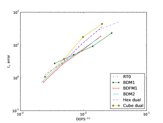
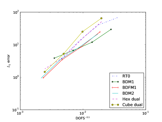
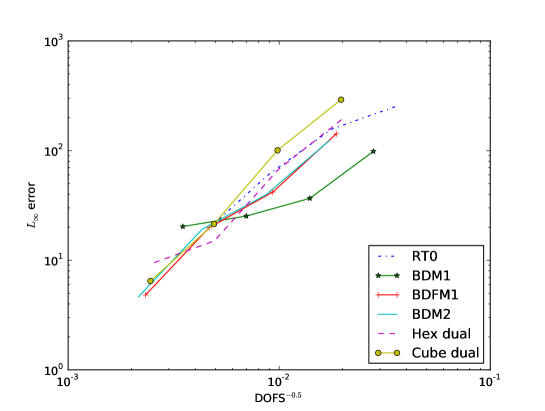
Figure 1: Tables showing numerical errors in the layer depth at 15 days for the standard “flow over a mountain” testcase, relative to a resolved pseudo-spectral solution, for various different finite element spaces.

5 Summary and outlook

In this paper, we used the finite element exterior calculus framework to develop two formulations for the shallow-water equations, a primal formulation that is defined on a single mesh where divergence is defined in the strong form but vorticity must be evaluated weakly using integration by parts, and a primal-dual formulation that makes use of a dual mesh where vorticity can also be computed in the strong form. Both of these formulations have a conserved diagnostic potential vorticity, that satisfies mass consistency i.e. constant $q$ stays constant. In the primal mesh case we are able to choose energy and enstrophy conserving mass and potential vorticity fluxes. Both formulations provide a way to control oscillations in the divergence-free component of the velocity field (the component that dominates in large scale balanced flow in the atmosphere) by ensuring that the potential vorticity remains mass-consistent and oscillation-free. In the primal-dual case this can be achieved since the potential vorticity is diagnosed on a discontinuous space where discontinuous Galerkin/finite volume methods can be used to provide stable shape-preserving potential vorticity fluxes. In the primal case, the potential vorticity is computed in a continuous finite element space, but streamline-upwind Petrov-Galerkin methods with discontinuity capturing are compatible with the framework and can be used to provide stable potential vorticity fluxes.

This work is part of the UK GungHo Dynamical Core project, which is a NERC/STFC collaboration between UK academics and the UK Met Office to design a dynamical core for the Unified Model that will perform well on the next generation of massively parallel supercomputers. In Phase 1 of the project, one of the main goals is to determine the horizontal discretisation that will be used, with the shallow-water equations on the sphere providing an environment to investigate this. The aim is to develop discretisations on a pseudouniform grid that have all of the desirable properties listed in the introduction, whilst maintaining the accuracy of the current model. Numerical accuracy is crucial since it reduces grid imprinting (structure in the numerical errors that reflects the structure of the grid, e.g. larger errors near the corners of a cubed sphere). This work opens up a number of possibilities that could be sufficiently accurate for operational use. In [14] it was shown that to avoid spurious mode branches it is necessary to select finite element spaces that have a 2:1 ratio of velocity DOFs to pressure DOFs, which suggests the BDFM1 space on triangles with an icosahedral mesh in the primal formulation or RT0 on quadrilaterals with a cubed sphere mesh in the primal-dual formulation. There is an argument to be made that spurious Rossby mode branches arising from increasing velocity DOFs relative to this ratio are not harmful since they have very low frequencies and will just be passively advected by the flow. This suggests the BDM1 space on triangles in the primal formulation or the RT0 space on hexagons in the primal-dual formulation, which both have a 3:1 ratio. The next steps in this work are to analyse the numerical convergence and dispersion relations of all of these schemes and to benchmark them against the usual suites of testcases and against solutions from the Unified Model formulation.

Acknowledgements

The authors would like to thank Thomas Dubos for suggesting to look at a primal-dual finite element formulation, Darryl Holm for useful guidance and comments on the paper, Andrew McRae for providing primal scheme testcase results, Hilary Weller for providing reference pseudospectral solutions, and the GungHo UK dynamical core team for interesting discussions and debate. This work is supported by the Natural Environment Research Council.

References

• Staniforth and Thuburn [2012] A. Staniforth, J. Thuburn, Horizontal grids for global weather and climate prediction models: a review, Q. J. Roy. Met. Soc 138 (2012) 1–26.
• Le Roux et al. [2005] D. Y. Le Roux, A. Sène, V. Rostand, E. Hanert, On some spurious mode issues in shallow-water models using a linear algebra approach, Ocean Modelling (2005) 83–94.
• Le Roux et al. [2007] D. Y. Le Roux, V. Rostand, B. Pouliot, Analysis of numerically induced oscillations in 2D finite-element shallow-water models part I: Inertia-gravity waves, SIAM Journal on Scientific Computing 29 (2007) 331–360.
• Le Roux and Pouliot [2008] D. Y. Le Roux, B. Pouliot, Analysis of numerically induced oscillations in two-dimensional finite-element shallow-water models part II: Free planetary waves, SIAM Journal on Scientific Computing 30 (2008) 1971–1991.
• Walters and Casulli [1998] R. Walters, V. Casulli, A robust, finite element model for hydrostatic surface water flows, Communications in Numerical Methods in Engineering 14 (1998) 931–940.
• Bonaventura and Ringler [2005] L. Bonaventura, T. Ringler, Analysis of discrete shallow-water models on geodesic Delaunay grids with C-type staggering, Mon. Weath. Rev. 133 (2005) 2351–2373.
• Danilov [2010] S. Danilov, On utility of triangular C-grid type discretization for numerical modeling of large-scale ocean flows, Ocean Dynamics 60 (2010) 1361–1369.
• Gassmann [2011] A. Gassmann, Inspection of hexagonal and triangular C-grid discretizations of the shallow water equations, J. Comp. Phys. 230 (2011) 2706–2721.
• Thuburn [2008] J. Thuburn, Numerical wave propagation on the hexagonal C-grid, J. Comp. Phys. 227 (2008) 5836–5858.
• Thuburn et al. [2009] J. Thuburn, T. D. Ringler, W. C. Skamarock, J. B. Klemp, Numerical representation of geostrophic modes on arbitrarily structured C-grids, J. Comput. Phys. 228 (2009) 8321–8335.
• Ringler et al. [2010] T. D. Ringler, J. Thuburn, J. B. Klemp, W. C. Skamarock, A unified approach to energy conservation and potential vorticity dynamics for arbitrarily-structured C-grids, Journal of Computational Physics 229 (2010) 3065–3090.
• Putman and Lin [2007] W. Putman, S.-J. Lin, Finite-volume transport on various cubed sphere grids, J. Comput. Phys. 227 (2007) 55–78.
• Thuburn and Cotter [2012] J. Thuburn, C. Cotter, A framework for mimetic discretization of the rotating shallow-water equations on arbitrary polygonal grids, SIAM J. Sci. Comp. (2012).
• Cotter and Shipton [2012] C. Cotter, J. Shipton, Mixed finite elements for numerical weather prediction, J. Comp. Phys. (2012).
• Arnold et al. [2006] D. Arnold, R. Falk, R. Winther, Finite element exterior calculus, homological techniques, and applications, Acta Numerica 15 (2006) 1–155.
• Hiptmair [2001a] R. Hiptmair, Discrete Hodge operators, Numerische Mathematik 90 (2001a) 265.
• Hiptmair [2001b] R. Hiptmair, Discrete Hodge operators : An algebraic perspective, Journal of electromagnetic waves and applications 15 (2001b) 343–344.
• Arnold et al. [2010] D. Arnold, R. Falk, R. Winther, Finite element exterior calculus: from hodge theory to numerical stability, Bull. Amer. Math. Soc.(NS) 47 (2010) 281–354.
• Marsden and Ratiu [1999] J. E. Marsden, T. S. Ratiu, Introduction to Mechanics and Symmetry, Springer, 1999.
• Holm [2011] D. D. Holm, Geometric Mechanics: Part II: Rotating, Translating and Rolling, Imperial College Press, 2011.
• Arakawa and Lamb [1981] A. Arakawa, V. Lamb, A potential enstrophy and energy conserving scheme for the shallow water equations, Monthly Weather Review 109 (1981) 18–36.
• Brezzi and Fortin [1991] F. Brezzi, M. Fortin, Mixed and hybrid finite element methods, Springer-Verlag New York, Inc., 1991.
• Bochev and Ridzal [2008] P. B. Bochev, D. Ridzal, Rehabilitation of the lowest-order raviart-thomas element on quadrilateral grids, SIAM Journal on Numerical Analysis 47 (2008) 487–507.
• Rognes et al. [2009] M. Rognes, R. Kirby, A. Logg, Efficient assembly of $H(\mathrm{div})$ and $H(\mathrm{curl})$ conforming finite elements, SISC 31 (2009) 4130–4151.
• Rognes et al. [2013] M. Rognes, D. Ham, C. Cotter, A. McRae, Automating the solution of PDEs on the sphere and other manifolds, 2013. Submitted.
• Arakawa and Hsu [1990] A. Arakawa, Y.-J. G. Hsu, Energy conserving and potential-enstrophy dissipating schemes for the shallow water equations, Monthly Weather Review 118 (1990) 1960–1969.
• Sadourny and Basdevant [1985] R. Sadourny, C. Basdevant, Parameterization of subgrid scale barotropic and baroclinic eddies in quasi-geostrophic models- anticipated potential vorticity method, Journal of the atmospheric sciences 42 (1985) 1353–1363.
• Brooks and Hughes [1982] A. N. Brooks, T. Hughes, Streamline upwind/Petrov-Galerkin formulations for convection dominated flows with particular emphasis on the incompressible Navier-Stokes equations, Computer Methods in Applied Mechanics and Engineering 32 (1982) 199 – 259.
• Shu [2009] C.-W. Shu, High order weighted essentially nonoscillatory schemes for convection dominated problems, SIAM review 51 (2009) 82–126.
• Thuburn [1997] J. Thuburn, A PV-based shallow-water model on a hexagonal-icosahedral grid, Monthly Weather Review 125 (1997) 2328–2347.
• Lipscomb and Ringler [2005] W. Lipscomb, T. Ringler, An incremental remapping transport scheme on a spherical geodesic grid, Monthly weather review 133 (2005) 2335–2350.
• Skamarock and Menchaca [2010] W. Skamarock, M. Menchaca, Conservative transport schemes for spherical geodesic grids: High-order reconstructions for forward-in-time schemes, Monthly Weather Review 138 (2010) 4497–4508.
• Fortin [1977] M. Fortin, An analysis of the convergence of mixed finite element methods, R.A.I.R.O., Anal. Numer. 11 (1977) 341–354.
• Arnold [2013] D. N. Arnold, Spaces of finite element differential forms, in: Analysis and Numerics of Partial Differential Equations, Springer, 2013, pp. 117–140.
• Cockburn and Shu [2001] B. Cockburn, C.-W. Shu, Runge-Kutta discontinuous Galerkin methods for convection-dominated problems, J. Sci. Comp. 16 (2001) 173–261.
• Buffa and Christiansen [2007] A. Buffa, S. Christiansen, A dual finite element complex on the barycentric refinement, Mathematics of Computation 76 (2007) 1743–1769.
• Christiansen [2008] S. Christiansen, A construction of spaces of compatible differential forms on cellular complexes, Mathematical Models and Methods in Applied Sciences 18 (2008) 739–757.
• Williamson et al. [1992] D. L. Williamson, J. B. Drake, J. J. Hack, R. Jakob, P. N. Swarztrauber, A standard test set for numerical approximations to the shallow water equations in spherical geometry, Journal of Computational Physics 102 (1992) 211–224.