Multi-gluon helicity amplitudes with one off-shell leg within high energy factorization

Abstract

Basing on the Slavnov-Taylor identities, we derive a new prescription to obtain gauge invariant tree-level scattering amplitudes for the process $g^{*}g\rightarrow N\,g$ within high energy factorization. Using the helicity method, we check the formalism up to several final state gluons, and we present analytical formulas for the the helicity amplitudes for $N=2$. We also compare the method with Lipatov’s effective action approach.

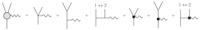
1 Introduction

The scientific plans of the Large Hadron Collider (LHC) span from tests of complex dynamics of the Standard Model [1] to searches for physics beyond it [2]. Quantum Chromodynamics (QCD) being a part of the Standard Model is the basic theory which is used to set up the calculational background for the collisions at LHC. Application of perturbative QCD relies on various factorization theorems which allow to decompose a given process into a long-distance part called parton density and a short distance hard process. In particular, for inclusive and jet production processes the appropriate long-distance part is realized in terms of various parton distribution functions. Here we will focus on high energy factorization [3] which applies when the energy scale involved in the scattering process is high. The evolution equations of high energy factorization sum up logarithms of energy accompanied by a coupling constant. Depending on the energy range and observable one uses: the BFKL [4, 5], BK [6, 7], CCFM [8, 9] or recently proposed new evolution equations accounting for both saturation and processes at large momentum transfers [10, 11].

The important ingredients of high energy factorization are unintegrated gluon densities, which depend not only on the longitudinal hadron momentum fraction but on the transversal momentum as well. They have to be convoluted with the hard process which is calculated with the initiating gluons being off-shell. In case of processes with non-gluonic final states, like $q$, $\bar{q}$ production for instance, the corresponding gauge invariant amplitudes can be calculated by applying so called high energy projectors, that resolve degrees of freedom relevant at high energies. The more general framework given in terms of Lipatov’s action [12] provides a prescription to calculate gauge invariant matrix elements in a general case for any partonic process initiated by off-shell gluons [13]. For recent studies and applications, we refer to [14, 15, 16, 17].

At present, various automatic numerical tools exist for the calculation of multi-gluon amplitudes for ordinary on-shell processes [18, 19, 20, 21, 22]. They operate on the amplitude level and use helicity methods, and thus are very efficient and universal. The present study is a first step aiming at similar methods for off-shell high energy amplitudes. We develop a new prescription for calculating gauge invariant high energy factorizable tree-level amplitudes with one of the gluons being off-shell. Our results turn out to be in agreement with results obtained using Lipatov’s action.

Our prescription can be summarized as follows. It is known [23] that the ordinary Feynman graphs contributing to an amplitude in an on-shell calculation are in general not sufficient to obtain gauge invariant results if any of the external legs are off-shell. Thus one usually needs to consider a larger on-shell process and disentangle the required gauge invariant off-shell amplitudes. Our approach is however different: we require the Slavnov-Taylor identities to hold for the off-shell connected amplitudes, which in turn induces the necessary contributions which by comparison to [23] can be interpreted as bremsstrahlung graphs introduced to restore gauge invariance. Our construction holds for any number of final state gluons and as an example we give a detailed derivation and discussion for the helicity amplitudes of the process $g^{*}g\rightarrow gg$. These amplitudes are the dominant contribution to forward-central di-jet production [24, 25, 26] and are of particular interest for testing parton densities at low longitudinal momentum fraction of the gluons with a special focus on saturation effects (for overview see [27] and for recent jet studies of these effects see [28]).

An extensive analyzis of tree-level multi-gluon helicity amplitudes in the high-energy limit was done also in Ref. [29]. There, the impact factors for $g^{*}g\rightarrow Ng$, $N\leq 3$ were disentangled at the amplitude level, however they do not correspond exactly to the kinematic situation considered in the present work.

The paper is organized as follows. Section 2 is introductory and is mainly devoted to set the notation. In particular, we overview high energy factorization focusing on the kinematic setup and we introduce the framework of color ordered helicity amplitudes which is used later in the paper. In Section 3 we identify the problem of gauge non-invariance of high energy factorization amplitudes and repair it using the Slavnov-Taylor identities. In Section 4 we describe analytical and numerical tests for gauge invariant helicity amplitudes, in particular we list the helicity amplitudes and their square for $g^{*}g\rightarrow gg$. We also cross check our result with those obtained by usage of Lipatov’s effective action. In the appendices we collect the color-ordered Feynman rules we needed in our construction of gauge invariant amplitudes as well as some technicalities on the Slavnov-Taylor identities.

2 Prerequisites and notation

2.1 High energy factorization

Our considerations of the off-shell amplitudes are embedded in the formalism of high energy factorization. Let us thus start with a brief recollection of this topic [3, 30, 31, 32].

The basic observation is that the cross section for a hadronic process can be decomposed at high energies into transversal momentum dependent parton densities and the hard partonic cross section with off-shell initial state partons. Thus, the intermediate object that appears is the amplitude for the process

$$g^{*}(k_{1})\,g^{*}(k_{2})\rightarrow X,$$ (1)

where $g^{*}$ denotes an off-shell gluon, and $X$ abbreviates the on-shell final state particles. In the considered high energy limit, the incident momenta are parametrized as

$$k_{1}^{\mu}\simeq\xi_{1}n_{a}^{\mu}+k_{1T}^{\mu},$$ (2)

$$k_{2}^{\mu}\simeq\xi_{2}n_{b}^{\mu}+k_{2T}^{\mu},$$ (3)

where $n_{a}$, $n_{b}$ are light-like momenta corresponding to the two incident hadrons $a$ and $b$. They satisfy $n_{a}\!\cdot\!k_{iT}=n_{b}\!\cdot\!k_{iT}=0$, and $k_{i}^{2}=k_{iT}^{2}=-\big{|}\vec{k}_{iT}\big{|}^{2}.$

In [3], for example, heavy quark production $g^{*}(k_{1})\,g^{*}(k_{2})\to Q\,\overline{Q}$ is considered. The amplitude is calculated by taking into account the usual tree-level Feynman graphs in the axial gauge with gauge vector $n^{\mu}=\alpha n_{a}^{\mu}+\beta n_{b}^{\mu}$. Then the gluon propagator is given by

$$D^{\mu\nu}\left(k\right)=S\left(k\right)\,d^{\mu\nu}\left(k,n\right),$$ (4)

with the scalar part

$$S\left(k\right)=\frac{-i}{k^{2}+i\epsilon}$$ (5)

and the transverse projector

$$d^{\mu\nu}\left(k,n\right)=\eta^{\mu\nu}-\frac{k^{\mu}n^{\nu}+k^{\nu}n^{\mu}}{k\!\cdot\!n}+n^{2}\frac{k^{\mu}k^{\nu}}{\left(k\!\cdot\!n\right)^{2}}.$$ (6)

Above $\eta^{\mu\nu}$ is the metric tensor and we have suppressed the color indices in $D^{\mu\nu}$. The off-shell legs include propagators, and are contracted with eikonal couplings defined as

$$\mathfrak{e}_{1}^{\mu}=\big{|}\vec{k}_{1T}\big{|}n_{a}^{\mu},$$ (7)

$$\mathfrak{e}_{2}^{\mu}=\big{|}\vec{k}_{2T}\big{|}n_{b}^{\mu}.$$ (8)

It is easy to check, that effectively an amputated amplitude is contracted with the following vector

$$-i\,\mathfrak{e}_{1}^{\mu}\,D_{\mu\nu}\left(k_{1}\right)=\frac{k_{T\,1}^{\mu}}{\xi_{1}\big{|}\vec{k}_{1T}\big{|}}$$ (9)

and similarly for $k_{2}$, which then is shown to lead to the correct result in the collinear limit. Furthermore, it is shown that the result is independent of the choice of gauge-vector, proving gauge invariance.

The above might be taken as a prescription to calculate amplitudes for arbitrary processes, but it will in general not lead to gauge-invariant results. To achieve the latter, additional contributions are needed. They are usually obtained by considering a larger, fully on-shell, process from which an amplitude for the off-shell process is extracted. The situation is somewhat simpler when one of the gluons, say $k_{2}$, reaches collinear limit, i.e. when $k_{2}^{2}\rightarrow 0$. In the following sections, we shall investigate such amplitudes for the process

$$g^{*}(k_{1})\,g(k_{2})\rightarrow g(k_{3})\ldots g(k_{N})$$ (10)

for an arbitrary number of final state gluons.

2.2 Color-ordered helicity amplitudes

Let us denote our purely gluonic tree-level amplitude with $N$ external gluons (one off-shell and $N-1$ on-shell) as $\mathcal{M}\left(\mathfrak{e}_{1},\varepsilon_{2},\ldots,\varepsilon_{N}\right)$. For the precise definition see Section 3. The polarization vectors of the on-shell gluons are denoted as $\varepsilon_{i}$. Whenever necessary, we shall indicate the polarization state explicitly using $\varepsilon_{i}^{(\lambda)}$ with $\lambda=\pm$. Following e.g. the Kleiss-Stirling construction [33], the polarization vectors can be defined in terms of the gluon momentum $k_{i}$ and an auxiliary light-like momentum $q_{i}$ satisfying $k_{i}\!\cdot\!q_{i}\neq 0$. Thus, whenever needed we use the notation $\varepsilon_{i}^{(\lambda)}(q_{i})$ to indicate explicitly what reference vector is used. The polarization vectors satisfy several conditions, of which we would like to highlight two, namely

$$\varepsilon_{i}^{(\lambda)}(q_{i})\!\cdot\!k_{i}=0,$$ (11)

$$\varepsilon_{i}^{(\lambda)}(q_{i})\!\cdot\!q_{i}=0.$$ (12)

When one changes the reference momentum, the corresponding polarization vector transforms as

$$\varepsilon_{i}^{\mu}\left(q^{\prime}_{i}\right)=\varepsilon_{i}^{\mu}\left(q_{i}\right)+\beta_{i}\left(q^{\prime}_{i},q_{i}\right)k_{i}^{\mu},$$ (13)

where the function $\beta_{i}$ depends on the precise representation for the polarization vectors. It is important to note, that as long as the amplitude $\mathcal{M}$ satisfies the Ward identity

$$\mathcal{M}\left(\mathfrak{e}_{1},\varepsilon_{2},\ldots,\varepsilon_{i-1},k_{i},\varepsilon_{i+1},\ldots,\varepsilon_{N}\right)=0,\quad i=2,\dots,N$$ (14)

the reference momenta can be freely changed, which has proved to be very useful for obtaining compact expressions for multi-gluon amplitudes (see e.g. [34] for a review). In explicit calculations we use the spinor representation for the polarization vectors

$$\varepsilon_{i}^{\mu\,\pm}\left(q_{i}\right)=\pm\frac{\left\langle q_{i}^{\mp}\right|\gamma^{\mu}\left|k_{i}^{\mp}\right\rangle}{\sqrt{2}\,\left\langle q_{i}^{\mp}|k_{i}^{\pm}\right\rangle},$$ (15)

where

$$\left\langle k_{i}^{-}|k_{j}^{+}\right\rangle=\overline{u}^{-}\left(k_{i}\right)u^{+}\left(k_{j}\right)\equiv\left\langle ij\right\rangle,$$ (16)

$$\left\langle k_{i}^{+}|k_{j}^{-}\right\rangle=\overline{u}^{+}\left(k_{i}\right)u^{-}\left(k_{j}\right)\equiv\left[ij\right]$$ (17)

and the positive-energy spinors with definite helicities are defined as $u^{\pm}\left(k_{i}\right)=\frac{1}{2}\left(1\pm\gamma_{5}\right)u\left(k_{i}\right)$. The spinor products can be explicitly calculated in the light-cone basis as

$$\left\langle ij\right\rangle=k_{\perp\,i}\,\sqrt{\frac{k^{+}_{j}}{k^{+}_{i}}}-k_{\perp\,j}\,\sqrt{\frac{k^{+}_{i}}{k^{+}_{j}}},$$ (18)

$$\left[ij\right]=-k^{*}_{\perp\,i}\sqrt{\frac{k^{+}_{j}}{k^{+}_{i}}}+k^{*}_{\perp\,j}\sqrt{\frac{k^{+}_{i}}{k^{+}_{j}}},$$ (19)

where $k^{\pm}=k^{0}\pm k^{3}$ and $k_{\perp}=k^{1}+ik^{2}$. We also use the following compact notation for spinor products with some $\Gamma/$ matrix insertion

$$\left\langle q^{-}\right|\Gamma/\left|k^{-}\right\rangle\equiv\left\langle q\right|\Gamma/\left|k\right],$$ (20)

$$\left\langle q^{+}\right|\Gamma/\left|k^{+}\right\rangle\equiv\left[q\right|\Gamma/\left|k\right\rangle.$$ (21)

Another important ingredient in this respect is the use of color-ordered amplitudes [35]. They are defined via

$$\mathcal{M}\left(\mathfrak{e}_{1},\varepsilon_{2},\ldots,\varepsilon_{N}\right)=\sum_{\underset{{\scriptstyle\textrm{permutations}}}{\textrm{non-cyclic}}}\mathrm{Tr}\left(t^{a_{1}}\ldots t^{a_{N}}\right)\,\mathcal{A}\left(\mathfrak{e}_{1},\varepsilon_{2},\ldots,\varepsilon_{N}\right),$$ (22)

where the summation is over all non-cyclic permutations of the color indices $\left\{a_{1},\ldots,a_{N}\right\}$ corresponding to the external gluons. The matrices $t^{a}$ are the generators of color $\mathrm{SU}\left(N_{c}\right)$ group normalized as $\mathrm{Tr}\left(t^{a}t^{b}\right)=\delta^{ab}$. Note, that the ordering of the arguments in $\mathcal{A}$ does matter and corresponds to the order of color matrices under the trace. There are several important properties of color-ordered amplitudes. Here we want to mention explicitly two of them. First, gauge invariance of $\mathcal{M}$ implies gauge invariance of $\mathcal{A}$. Second, the full amplitude squared is given by

$$\sum_{\mathrm{colors}}\left|\mathcal{M}\left(\mathfrak{e}_{1},\varepsilon_{2},\ldots,\varepsilon_{N}\right)\right|^{2}=N_{c}^{N-2}\left(N_{c}^{2}-1\right)\!\!\!\!\!\sum_{\underset{{\scriptstyle\textrm{permutations}}}{\textrm{non-cyclic}}}\left|\mathcal{A}\left(\mathfrak{e}_{1},\varepsilon_{2},\ldots,\varepsilon_{N}\right)\right|^{2}\\ +\mathcal{O}\left(N_{c}^{N-2}\right),$$ (23)

where the contribution $\mathcal{O}\left(N_{c}^{N-2}\right)$ vanishes for $N\leq 5$.

3 Amplitudes with one off-shell leg

\psfragscanon\psfrag{1}{$k_{2}$}\psfrag{2}{$k_{1}$}\psfrag{3}{$k_{3}$}\psfrag{4}{$k_{N}$}\includegraphics[width=85.35826pt]{figure1}

Figure 1: The color-ordered amplitude $\mathcal{A}\left(\mathfrak{e}_{1},\varepsilon_{2},\ldots,\varepsilon_{N}\right)$ defined in the main text. The special external vertex corresponds to eikonal coupling $\mathfrak{e}_{1}^{\mu}=\big{|}\vec{k}_{T}\big{|}n_{a}^{\mu}$, while all the other external lines are amputated and contracted with the corresponding polarization vectors. The arrows show the choice of the momenta signs, while the vertical dots stand for the remaining external gluons.

The subject of our investigations are gluonic amplitudes with one off-shell leg, Eq. (10). More precisely, they are obtained from the corresponding momentum space Green function by means of the following reduction formula

$$\mathcal{M}\left(\mathfrak{e}_{1},\varepsilon_{2},\ldots,\varepsilon_{N}\right)=\lim_{k_{1}\cdot n_{a}\rightarrow 0}\,\lim_{k_{2}^{2},\ldots,k_{N}^{2}\rightarrow 0}\,\mathfrak{e}_{1}^{\mu_{1}}\varepsilon_{2}^{\mu_{2}}\ldots\varepsilon_{N}^{\mu_{N}}\,\\ S^{-1}\left(k_{2}\right)\ldots S^{-1}\left(k_{N}\right)\tilde{G}_{\mu_{1}\ldots\mu_{N}}\left(k_{1},\ldots,k_{N}\right),$$ (24)

where the scalar propagators are defined in Eg. (5) and $\tilde{G}$ is momentum space Green function defined as usual, by Fourier transforming the vacuum matrix element of a time ordered product of gluon fields. Note, that the first limit is a formal way of implementing the kinematic condition (2). The amplitude defined in Eq. (24) is incidentally not gauge invariant, see the discussion below.

Let us remark, that for ordinary, completely on-shell amplitudes the common practice is to amputate the external gluon legs together with potential projectors (6), if one uses axial gauge for $\tilde{G}$. In other words, in such case we can choose different gauges for the internal (off-shell) and the external (on-shell) lines and the scattering amplitude does not depend on this choice. It is of course also possible to do so at intermediate stages of a calculation when dealing with gauge-dependent quantities, however one has to be consistent, as different gauge-dependent pieces are to eventually compose a gauge invariant object.

In this spirit, in what follows we work in the axial gauge with $n_{a}$ being the gauge vector for internal off-shell lines (including line $k_{1}$) while the external on-shell gluons are reduced in the Feynman gauge, unless otherwise specified. That is, any vertex adjacent to an external on-shell gluon is contracted with the corresponding polarization vector directly.

In what follows, we consider a color-ordered amplitude for some specific color ordering, say $\left(a_{1},a_{2},\ldots,a_{N}\right)$, where $a_{i}$ is the color quantum number of the gluon with momentum $k_{i}$. As follows from (24), the off-shell leg $k_{1}$ contains the full propagator and is contracted with the eikonal vertex $\mathfrak{e}_{1}$ defined in Eq. (7), which we graphically denote as a circle with a cross (Fig. 1). According to Section 2.2, the amplitude under consideration is denoted as $\mathcal{A}\left(\mathfrak{e}_{1},\varepsilon_{2},\ldots,\varepsilon_{N}\right)$. For simplicity, we choose

$$k_{1}^{\mu}=n_{a}^{\mu}+k_{T}^{\mu}$$ (25)

as the momentum of the off-shell gluon (i.e. we absorb $\xi$ into $n_{a}$ in Eq. (2)).

Because of the off-shell external leg, taking into account the usual tree-level Feynman graphs and using the usual Feynman rules will not lead to a gauge invariant amplitude. In particular, it will not satisfy the usual Ward identities, i.e.

$$\mathcal{A}\left(\mathfrak{e}_{1},\varepsilon_{2},\ldots,\varepsilon_{i-1},k_{i},\varepsilon_{i+1},\ldots,\varepsilon_{N}\right)\neq 0,\quad i=2,\ldots,N,$$ (26)

which are indispensable for the calculation of helicity amplitudes. Indeed, it is not the Ward identity of the above form that follows from the local gauge invariance. Rather, one should consider the non-abelian Slavnov-Taylor (S-T) identites, which relate the amplitude $\mathcal{A}$ with nonphysical polarization (i.e. insertion of $k_{i}$) and the corresponding diagrams with ghosts. In the next section, we shall wander this path to construct a new amplitude

$$\tilde{\mathcal{A}}\left(\mathfrak{e}_{1},\varepsilon_{2},\ldots,\varepsilon_{N}\right)=\mathcal{A}\left(\mathfrak{e}_{1},\varepsilon_{2},\ldots,\varepsilon_{N}\right)+\mathcal{W}\left(\mathfrak{e}_{1},\varepsilon_{2},\ldots,\varepsilon_{N}\right),$$ (27)

such that

$$\tilde{\mathcal{A}}\left(\mathfrak{e}_{1},\varepsilon_{2},\ldots,\varepsilon_{i-1},k_{i},\varepsilon_{i+1},\ldots,\varepsilon_{N}\right)=0,\quad i=2,\ldots,N.$$ (28)

Since we provide a prescription to calculate $\tilde{\mathcal{A}}\left(\mathfrak{e}_{1},\varepsilon_{2},\ldots,\varepsilon_{N}\right)$ in a specific gauge, the fact that it satisfies Eq. (28) is an indication that it is the correct gauge invariant result. Moreover, we show in Appendix E that (27) posseses correct collinear and soft behaviour in the corresponding limits.

3.1 Restoration of gauge invariance

In what follows, we skip the first argument (corresponding to the off-shell leg) in the color-ordered amplitude $\mathcal{A}$, i.e. we write $\mathcal{A}\left(\mathfrak{e}_{1},\varepsilon_{2},\ldots,\varepsilon_{N}\right)\equiv\mathcal{A}\left(\varepsilon_{2},\ldots,\varepsilon_{N}\right)$ for compactness. In the gauge we specified above, our solution for the ‘gauge restoring’ amplitude $\mathcal{W}$ reads

$$\mathcal{W}\left(\varepsilon_{2},\ldots,\varepsilon_{N}\right)=\left(-\frac{g}{\sqrt{2}}\right)^{N-2}\frac{-\big{|}\vec{k}_{T}\big{|}\,\varepsilon_{2}\!\cdot\!n_{a}\ldots\varepsilon_{N}\!\cdot\!n_{a}}{k_{2}\!\cdot\!n_{a}\,\left(k_{2}-k_{3}\right)\!\cdot\!n_{a}\,\dots\left(k_{2}-\ldots-k_{N-1}\right)\!\cdot\!n_{a}}.$$ (29)

The above formula can be interpreted as a straight Wilson line along $n_{a}$ with the external gluons attached to it, however such an interpretation is beyond the scope of this paper and shall be analyzed elsewhere.

As already mentioned, according to the S-T identities, the insertion of $k_{i}$ generates additional gauge terms on the r.h.s of (26). We shall see that by controlling those terms one can indeed reconstruct $\mathcal{W}$. The S-T identities in different gauges together with some less common issues are recollected in Appendix A.

Let us consider first the (color-ordered) momentum space Green function, from which our amplitude is obtained according to the reduction procedure (24). Since we have chosen the Feynman gauge for the external on-shell lines, the relevant S-T identity involves the space-time derivative of the fields and in turn translates into a momentum insertion as in (26), c.f. (74).

A)

\psfragscanon\psfrag{1}{$=$}\psfrag{2}{$+$}\psfrag{4}{$+\,\dots$}\psfrag{3}{$+$}\psfrag{5}{$+\,\dots$}\includegraphics[width=284.52756pt]{figure2}

B)

\psfragscanon\psfrag{1}{$=$}\psfrag{2}{$+$}\psfrag{3}{$\!\!\!=$}\includegraphics[width=284.52756pt]{figure3}

Figure 2: A) The Slavnov-Taylor identity for the Green function (with external propagators) contracted with $k_{2}$. The contraction is graphically denoted by the arrow transforming to a solid line (see Appendix B). The dashed lines with arrows are standard notation for ghosts. Horizontal dots denote analogous diagrams for the rest of external legs. B) Application of the identity for the amplitude for a process with $N-1$ on-shell gluons and one off-shell leg contracted with an eikonal vertex. Most of the gauge diagrams vanish as described in the main text, but not all due to the off-shellness of $k_{1}$.

The S-T identities for the Green functions are most conveniently given in graphical form. We show an example in Fig. 2A for the contraction with $k_{2}$. It generates a set of diagrams involving ghosts and picks out a ghost-gluon vertex (see (75) in Appendix A) without an external propagator. The ghosts propagating to the shaded blob, which is assumed to be calculated in the axial gauge, may need some explanation. Let us note that the ghosts can be introduced also in the axial gauge but they decouple for ordinary processes, see e.g. [36] and Appendix A for additional explanations. The ghost-gluon coupling is proportional to $n_{a}^{\mu}$ and is transverse to the gluon propagator in the axial gauge $n_{a}^{\mu}d_{\mu\nu}\left(k,n_{a}\right)=0$, thus any internal gluon cannot be coupled to a ghost. In our case, however, a ghost can couple to external on-shell gluons, which are taken in the Feynman gauge and for which the projector $d_{\mu\nu}$ is absent.

When going from the Green function to the amplitude $\mathcal{A}$ most of the additional gauge diagrams vanish (Fig. 2B), either due to the transversality condition (11), or because the residue at the physical pole is zero (due to the lack of the external propagator, c.f. the reduction formula (24)). However, since $k_{1}$ is off-shell eventually one term survives, namely the one with the ghost-gluon vertex with the amputated external line (the second term of BRST transformation vertex (75)) contracted with the eikonal coupling. Note, that the first term in the middle in Fig. 2B vanishes due to the relation $k_{1}\!\cdot\!n_{a}=0$.

\psfragscanon\psfrag{1}{$k_{1}$}\psfrag{2}{$k_{2}$}\psfrag{3}{$k_{3}$}\psfrag{4}{$k_{4}$}\includegraphics[width=184.9429pt]{figure4}

Figure 3: The diagrams contributing to the Slavnov-Taylor identity for the color-ordered amplitude $\mathcal{A}\left(\mathfrak{e}_{1},\varepsilon_{2},\varepsilon_{3},\varepsilon_{4}\right)$, corresponding to the the process $g^{*}g\rightarrow gg$. We show the momentum flow in the leftmost diagram only. The right diagram is zero if the axial gauge with $n_{a}$ gauge vector is chosen.

In order to illustrate the above statements, let us look at the specific realization of the gauge diagrams from Fig. 2B for the simplest process $g^{*}g\rightarrow gg$. We display the diagrams in Fig. 3 for the color-ordered amplitude. Since we work in the axial gauge for the internal lines, no gluon line can attach to a ghost unless it is an external line. There is only one possible diagram with a triple-gluon coupling in which it is connected to the eikonal vertex (right diagram in Fig. 3). But this diagram is also zero, since we have chosen $n_{a}$ as the gauge vector.

The remaining gauge diagrams can easily be calculated and one can explicitly check the S-T identities (we checked it also for a general axial gauge with gauge vector $n\neq n_{a}$). For instance, for the left diagram from Fig. 3 we obtain using the Feynman rules collected in Appendix B

$$\frac{g^{2}}{2}\big{|}\vec{k}_{T}\big{|}\,\frac{n_{a}\!\cdot\!\varepsilon_{3}\,n_{a}\!\cdot\!\varepsilon_{4}}{\left(k_{2}-k_{3}\right)\!\cdot\!n_{a}}\equiv\mathcal{W}_{1}\left(k_{2},\varepsilon_{3},\varepsilon_{4}\right).$$ (30)

The arguments of $\mathcal{W}_{1}$ are chosen in this way for further convenience and show what leg is contracted with the momentum in the corresponding S-T relation.

\psfragscanon\psfrag{1}{$\mathcal{W}_{2a}$}\psfrag{2}{$\mathcal{W}_{2b}$}\psfrag{3}{$\mathcal{W}_{3}$}\includegraphics[width=256.0748pt]{figure5}

Figure 4: The color-ordered gauge diagrams for the contractions of the amplitude $\mathcal{A}\left(\varepsilon_{2},\varepsilon_{3},\varepsilon_{4}\right)$ with the external momenta; here $\mathcal{W}_{2a}$ and $\mathcal{W}_{2b}$ correspond to $\mathcal{A}\left(\varepsilon_{2},k_{3},\varepsilon_{4}\right)$, while $\mathcal{W}_{3}$ corresponds to $\mathcal{A}\left(\varepsilon_{2},\varepsilon_{3},k_{4}\right)$. The momentum flow is the same as in Fig. 3.

We can derive analogous identities involving contractions for different external legs. The corresponding gauge diagrams are depicted in Fig. 4. Using analogous naming convention as in Eq. (30) they read

$$\mathcal{W}_{2a}\left(\varepsilon_{2},k_{3},\varepsilon_{4}\right)=\frac{g^{2}}{2}\big{|}\vec{k}_{T}\big{|}\,\frac{n_{a}\!\cdot\!\varepsilon_{2}\,n_{a}\!\cdot\!\varepsilon_{4}}{\left(k_{1}+k_{2}\right)\!\cdot\!n_{a}},$$ (31)

$$\mathcal{W}_{2b}\left(\varepsilon_{2},k_{3},\varepsilon_{4}\right)=\frac{g^{2}}{2}\big{|}\vec{k}_{T}\big{|}\,\frac{n_{a}\!\cdot\!\varepsilon_{2}\,n_{a}\!\cdot\!\varepsilon_{4}}{\left(k_{1}-k_{4}\right)\!\cdot\!n_{a}},$$ (32)

$$\mathcal{W}_{3}\left(\varepsilon_{2},\varepsilon_{3},k_{4}\right)=-\frac{g^{2}}{2}\big{|}\vec{k}_{T}\big{|}\,\frac{n_{a}\!\cdot\!\varepsilon_{2}\,n_{a}\!\cdot\!\varepsilon_{3}}{\left(k_{1}+k_{2}\right)\!\cdot\!n_{a}}.$$ (33)

An immediate observation is that the gauge diagrams are proportional to $\big{|}\vec{k}_{T}\big{|}$, thus they vanish when all the particles become on-shell; consequently the l.h.s. of (26) equals to zero in that limit.

The ‘gauge restoring’ amplitude $\mathcal{W}$ in (27) can be obtained using the above results. First, we define $\mathcal{W}_{x}\left(\varepsilon_{2},\varepsilon_{3},\varepsilon_{4}\right)$ (note the arguments) for $x=1,2a,2b,3$ by multiplying the external ghost lines with the longitudinal projections of the corresponding polarization vectors. More precisely, we multiply the ghost leg $i$ with $\varepsilon_{i}\!\cdot\!n_{a}/k_{i}\!\cdot\!n_{a}$. Hence we have

$$\mathcal{W}_{1}\left(\varepsilon_{2},\varepsilon_{3},\varepsilon_{4}\right)=-\mathcal{W}_{3}\left(\varepsilon_{2},\varepsilon_{3},\varepsilon_{4}\right)=\frac{g^{2}}{2}\big{|}\vec{k}_{T}\big{|}\,\frac{n_{a}\!\cdot\!\varepsilon_{2}\,n_{a}\!\cdot\!\varepsilon_{3}\,n_{a}\!\cdot\!\varepsilon_{4}}{k_{2}\!\cdot\!n_{a}\,k_{4}\!\cdot\!n_{a}},$$ (34)

$$\mathcal{W}_{2a}\left(\varepsilon_{2},\varepsilon_{3},\varepsilon_{4}\right)=\frac{g^{2}}{2}\big{|}\vec{k}_{T}\big{|}\,\frac{n_{a}\!\cdot\!\varepsilon_{2}\,n_{a}\!\cdot\!\varepsilon_{3}\,n_{a}\!\cdot\!\varepsilon_{4}}{k_{2}\!\cdot\!n_{a}\,k_{3}\!\cdot\!n_{a}},$$ (35)

$$\mathcal{W}_{2b}\left(\varepsilon_{2},\varepsilon_{3},\varepsilon_{4}\right)=-\frac{g^{2}}{2}\big{|}\vec{k}_{T}\big{|}\,\frac{n_{a}\!\cdot\!\varepsilon_{2}\,n_{a}\!\cdot\!\varepsilon_{3}\,n_{a}\!\cdot\!\varepsilon_{4}}{k_{3}\!\cdot\!n_{a}\,k_{4}\!\cdot\!n_{a}},$$ (36)

Then, we define

$$\mathcal{W}\left(\varepsilon_{2},\varepsilon_{3},\varepsilon_{4}\right)=\mathcal{W}_{1}\left(\varepsilon_{2},\varepsilon_{3},\varepsilon_{4}\right)+\mathcal{W}_{2a}\left(\varepsilon_{2},\varepsilon_{3},\varepsilon_{4}\right)\\ +\mathcal{W}_{2b}\left(\varepsilon_{2},\varepsilon_{3},\varepsilon_{4}\right)+\mathcal{W}_{3}\left(\varepsilon_{2},\varepsilon_{3},\varepsilon_{4}\right).$$ (37)

Adding the diagrams, we recover the result anticipated in Eq. (29) for $N=4$

$$\mathcal{W}\left(\varepsilon_{2},\varepsilon_{3},\varepsilon_{4}\right)=-\frac{g^{2}}{2}\big{|}\vec{k}_{T}\big{|}\,\frac{n_{a}\!\cdot\!\varepsilon_{2}\,n_{a}\!\cdot\!\varepsilon_{3}\,n_{a}\!\cdot\!\varepsilon_{4}}{k_{2}\!\cdot\!n_{a}\,k_{4}\!\cdot\!n_{a}}.$$ (38)

It is straightforward to check that indeed (28) is satisfied with this choice of $\mathcal{W}$. It is a general property of $\mathcal{W}$ in our choice of gauge, that the sum of the diagrams with ghosts (and further replaced by longitudinal gluon polarization) collapses to single terms. The complete proof of Eq. (29) for any number of gluons is relegated to Appendix D.

We want to close this section with the following remark. Note that if we choose the reference momentum for any of the polarization vectors to be $n_{a}$, the ‘gauge restoring’ amplitude is zero

$$\mathcal{W}\left(\varepsilon_{2},\ldots,\varepsilon_{i-1},\varepsilon_{i}\left(n_{a}\right),\varepsilon_{i+1},\ldots,\varepsilon_{N}\right)=0$$ (39)

for any leg $i$. It follows from the property of polarization vectors (12). Let us now note, that we can always project a polarization vector with any reference momentum $q_{i}$ to the one with $n_{a}$ using

$$\varepsilon_{i}^{\mu}\left(q_{i}\right)d_{\mu}^{\nu}\left(k_{i},n_{a}\right)=\varepsilon_{i}^{\nu}\left(n_{a}\right),$$ (40)

with $d^{\mu\nu}\left(k_{i},n_{a}\right)$ defined in (6). It follows simply from the transversality condition $n_{a}\!\cdot\!d\left(k_{i},n_{a}\right)=0$. The above remark leads to a conclusion that the gauge invariant amplitude (27) can be written as

$$\tilde{\mathcal{A}}\left(\varepsilon_{2},\ldots,\varepsilon_{N}\right)=\mathcal{A}\left(\varepsilon_{2},\ldots,\varepsilon_{i-1},d\left(k_{i},n_{a}\right)\!\cdot\!\varepsilon_{i},\varepsilon_{i+1},\ldots,\varepsilon_{N}\right),$$ (41)

that is one can apply the transverse projector $d^{\mu\nu}\left(k_{i},n_{a}\right)$ to any number (at least one) of external on-shell legs. In particular, one can apply the projectors to all on-shell legs. Then, (28) is trivially satisfied for any $i$, since $k_{i}\!\cdot\!d\left(k_{i},n_{a}\right)=0$ for $k_{i}^{2}=0$. Thus one could have the impression that it is also possible for any gauge vector $n\neq n_{a}$, as the projector remains transverse to $k_{i}$ and the ‘naive’ Ward identity is satisfied. This however does not mean that such amplitude is gauge invariant – we relegate this issue to Appendix C.

4 Analytical and numerical tests

4.1 Numerical tests

We tested (28) numerically up to $N=12$, calculating $\mathcal{A}$ with numerical Berends-Giele recursion [37]. We also tested (28) for color-dressed amplitudes up to $N=8$, by calculating $\mathcal{M}$ in the color-flow representation following the method of [38, 39]. The color-dressed version of $\mathcal{W}$ was calculated by straightforward multiplication with the color-dependent factor and summation over the necessary permutations, i.e. following Eq. (22) with the color-factor in the color-flow representation [40, 41].

4.2 Analytic expressions for $g^{*}g\rightarrow gg$

Let us start with the amplitude with full dependence on polarization vectors. Defining

$$\varepsilon_{1}^{\mu}=\frac{k_{T}^{\mu}}{\big{|}\vec{k}_{T}\big{|}}$$ (42)

we get explicitly for color-ordering $\left(a_{1},a_{2},a_{3},a_{4}\right)$

$$\tilde{\mathcal{A}}\left(\varepsilon_{2},\varepsilon_{3},\varepsilon_{4}\right)=\tilde{\mathcal{A}}\left(\varepsilon_{4},\varepsilon_{3},\varepsilon_{2}\right)=\frac{g^{2}}{2\,k_{2}\!\cdot\!k_{3}k_{3}\!\cdot\!k_{4}k_{2}\!\cdot\!n_{a}k_{4}\!\cdot\!n_{a}}\\ (n_{a}\!\cdot\!\varepsilon_{3}(k_{2}\!\cdot\!k_{3}k_{3}\!\cdot\!\varepsilon_{4}k_{4}\!\cdot\!n_{a}\varepsilon_{1}\!\cdot\!\varepsilon_{2}+k_{2}\!\cdot\!n_{a}k_{3}\!\cdot\!k_{4}k_{3}\!\cdot\!\varepsilon_{2}\varepsilon_{1}\!\cdot\!\varepsilon_{4})k_{1}^{2}\\ +k_{4}\!\cdot\!n_{a}(k_{2}\!\cdot\!n_{a}((k_{2}\!\cdot\!k_{3}k_{4}\!\cdot\!\varepsilon_{3}\,\mathfrak{t}-k_{3}\!\cdot\!k_{4}(k_{2}\!\cdot\!\varepsilon_{3}\,\mathfrak{r}+2k_{2}\!\cdot\!k_{3}\varepsilon_{1}\!\cdot\!\varepsilon_{3}))\varepsilon_{2}\!\cdot\!\varepsilon_{4}\\ +k_{2}\!\cdot\!k_{3}(2(k_{1}\!\cdot\!\varepsilon_{4}k_{2}\!\cdot\!\varepsilon_{3}\varepsilon_{1}\!\cdot\!\varepsilon_{2}-k_{1}\!\cdot\!\varepsilon_{3}(k_{2}\!\cdot\!\varepsilon_{4}\varepsilon_{1}\!\cdot\!\varepsilon_{2}+k_{1}\!\cdot\!\varepsilon_{2}\varepsilon_{1}\!\cdot\!\varepsilon_{4})\\ +k_{1}\!\cdot\!\varepsilon_{2}(k_{3}\!\cdot\!\varepsilon_{4}\varepsilon_{1}\!\cdot\!\varepsilon_{3}-k_{2}\!\cdot\!\varepsilon_{3}\varepsilon_{1}\!\cdot\!\varepsilon_{4}))-(2\mathfrak{u}_{13}\!\cdot\!\varepsilon_{2}-k_{3}\!\cdot\!\varepsilon_{2}\,\mathfrak{t})\varepsilon_{3}\!\cdot\!\varepsilon_{4})\\ +k_{3}\!\cdot\!k_{4}(2k_{2}\!\cdot\!\varepsilon_{3}\,\mathfrak{s}_{24}+k_{3}\!\cdot\!\varepsilon_{2}(2\mathfrak{s}_{34}-\mathfrak{r}\,\varepsilon_{3}\!\cdot\!\varepsilon_{4})))\\ +k_{2}\!\cdot\!k_{3}((k_{4}\!\cdot\!\varepsilon_{3}n_{a}\!\cdot\!\varepsilon_{4}+k_{3}\!\cdot\!n_{a}\varepsilon_{3}\!\cdot\!\varepsilon_{4})\mathfrak{p}\!\cdot\!\varepsilon_{2}-k_{1}\!\cdot\!\varepsilon_{1}k_{1}\!\cdot\!\varepsilon_{2}k_{3}\!\cdot\!\varepsilon_{4}n_{a}\!\cdot\!\varepsilon_{3}))\\ +k_{2}\!\cdot\!n_{a}(k_{3}\!\cdot\!k_{4}(k_{2}\!\cdot\!\varepsilon_{3}n_{a}\!\cdot\!\varepsilon_{2}\varepsilon_{1}\!\cdot\!\varepsilon_{4}k_{1}^{2}-k_{1}\!\cdot\!\varepsilon_{1}k_{1}\!\cdot\!\varepsilon_{4}(k_{2}\!\cdot\!\varepsilon_{3}n_{a}\!\cdot\!\varepsilon_{2}+k_{3}\!\cdot\!\varepsilon_{2}n_{a}\!\cdot\!\varepsilon_{3}))\\ +\varepsilon_{2}\!\cdot\!\varepsilon_{3}(k_{4}\!\cdot\!n_{a}((\mathfrak{t}\,k_{1}\!\cdot\!k_{3}-2k_{3}\!\cdot\!k_{4}k_{3}\!\cdot\!\varepsilon_{1})k_{3}\!\cdot\!\varepsilon_{4}+2k_{3}\!\cdot\!k_{4}\mathfrak{u}_{13}\!\cdot\!\varepsilon_{4})\\ +k_{3}\!\cdot\!k_{4}k_{3}\!\cdot\!n_{a}\mathfrak{p}\!\cdot\!\varepsilon_{4}))+k_{1}\!\cdot\!\varepsilon_{1}\,\varepsilon_{2}\!\cdot\!n_{a}\,\varepsilon_{3}\!\cdot\!n_{a}\,\varepsilon_{4}\!\cdot\!n_{a}\,k_{2}\!\cdot\!k_{3}\,k_{3}\!\cdot\!k_{4})$$ (43)

where we have used

$$\mathfrak{p}^{\alpha}=k_{1}\!\cdot\!\varepsilon_{1}\,k_{1}^{\alpha}-k_{1}^{2}\varepsilon_{1}^{\alpha},$$ (44)

$$\mathfrak{r}=k_{1}\!\cdot\!\varepsilon_{1}+2k_{2}\!\cdot\!\varepsilon_{1}-2k_{3}\!\cdot\!\varepsilon_{1},$$ (45)

$$\mathfrak{s}_{ij}=k_{1}^{\alpha}\varepsilon_{1}^{\beta}\left(\varepsilon_{i\,\alpha}\varepsilon_{j\,\beta}-\varepsilon_{i\,\beta}\varepsilon_{j\,\alpha}\right),$$ (46)

$$\mathfrak{t}=k_{1}\!\cdot\!\varepsilon_{1}+2k_{2}\!\cdot\!\varepsilon_{1},$$ (47)

$$\mathfrak{u}_{ij}^{\alpha}=k_{i}^{\alpha}k_{j}\!\cdot\!\varepsilon_{1}-k_{i}\!\cdot\!k_{j}\varepsilon_{1}^{\alpha}.$$ (48)

We have not used any particular reference momenta for the polarization vectors – by applying different choices the above expression can be simplified. Note, that we are allowed to play with the reference momenta as the above amplitude is gauge invariant; the $\mathcal{W}$ piece is already included above (the last term). The other color-ordered amplitudes are obtained by exchanging the relevant polarization vectors and momenta in the expression above.

Using the spinor helicity formalism one can calculate those amplitudes explicitly for different helicity combinations. For this purpose it proves most convenient to choose $n_{a}$ as a reference vector for each of the on-shell gluons. Labeling spinors associated with the light-like momenta $n_{a}$, $k_{2}$, $k_{3}$, $k_{4}$ with $a$, $2$, $3$, $4$ respectively, and further using the notation introduced in Section 2.2 (see also [35]), we find

$$\tilde{\mathcal{A}}(\varepsilon_{2}^{-}(n_{a}),\varepsilon_{3}^{-}(n_{a}),\varepsilon_{4}^{-}(n_{a})) =0,$$ (49)

$$\tilde{\mathcal{A}}(\varepsilon_{2}^{+}(n_{a}),\varepsilon_{3}^{+}(n_{a}),\varepsilon_{4}^{+}(n_{a})) =0,$$ (50)

$$\tilde{\mathcal{A}}(\varepsilon_{2}^{-}(n_{a}),\varepsilon_{3}^{-}(n_{a}),\varepsilon_{4}^{+}(n_{a})) =\frac{g^{2}}{\sqrt{2}}\,\frac{[3|k/_{T}|a\rangle}{\big{|}\vec{k}_{T}\big{|}}\,\frac{[4a]^{3}}{[3a][a2][23][34]},$$ (51)

$$\tilde{\mathcal{A}}(\varepsilon_{2}^{+}(n_{a}),\varepsilon_{3}^{+}(n_{a}),\varepsilon_{4}^{-}(n_{a})) =\frac{g^{2}}{\sqrt{2}}\,\frac{\langle a|k/_{T}|3]}{\big{|}\vec{k}_{T}\big{|}}\,\frac{\langle 4a\rangle^{3}}{\langle a3\rangle\langle a2\rangle\langle 23\rangle\langle 34\rangle},$$ (52)

$$\tilde{\mathcal{A}}(\varepsilon_{2}^{-}(n_{a}),\varepsilon_{3}^{+}(n_{a}),\varepsilon_{4}^{+}(n_{a})) =\frac{g^{2}}{\sqrt{2}}\,\frac{\langle a|k/_{T}|3]}{\big{|}\vec{k}_{T}\big{|}}\,\frac{\langle a2\rangle^{3}}{\langle a3\rangle\langle 23\rangle\langle 34\rangle\langle 4a\rangle},$$ (53)

$$\tilde{\mathcal{A}}(\varepsilon_{2}^{+}(n_{a}),\varepsilon_{3}^{-}(n_{a}),\varepsilon_{4}^{-}(n_{a})) =\frac{g^{2}}{\sqrt{2}}\,\frac{[3|k/_{T}|a\rangle}{\big{|}\vec{k}_{T}\big{|}}\,\frac{[a2]^{3}}{[3a][23][34][4a]},$$ (54)

$$\tilde{\mathcal{A}}(\varepsilon_{2}^{-}(n_{a}),\varepsilon_{3}^{+}(n_{a}),\varepsilon_{4}^{-}(n_{a})) =\frac{g^{2}}{\sqrt{2}}\,\frac{[3|k/_{T}|a\rangle}{\big{|}\vec{k}_{T}\big{|}}\,\frac{[3a]^{3}}{[a2][23][34][4a]},$$ (55)

$$\tilde{\mathcal{A}}(\varepsilon_{2}^{+}(n_{a}),\varepsilon_{3}^{-}(n_{a}),\varepsilon_{4}^{+}(n_{a})) =\frac{g^{2}}{\sqrt{2}}\,\frac{\langle a|k/_{T}|3]}{\big{|}\vec{k}_{T}\big{|}}\,\frac{\langle a3\rangle^{3}}{\langle a2\rangle\langle 23\rangle\langle 34\rangle\langle 4a\rangle}.$$ (56)

All momenta are assumed to be incoming in the formulas above. In what follows we skip the reference momenta indication in the amplitudes.

We may decompose $k_{T}^{\mu}$ in terms of $k_{3}^{\mu}$ and another light-like momentum $p^{\mu}$ following

$$k_{T}^{\mu}=p^{\mu}+\frac{k_{T}^{2}}{2k_{T}\!\cdot\!k_{3}}\,k_{3}^{\mu}\leavevmode\nobreak\ .$$

References

- Salgado et al. [2012] C. Salgado, J. Alvarez-Muniz, F. Arleo, N. Armesto, M. Botje, et al., J.Phys.G G39, 015010 (2012), 1105.3919
- Albrow et al. [2009] M. Albrow et al. (FP420 R and D Collaboration), JINST 4, T10001 (2009), 0806.0302
- Catani et al. [1991a] S. Catani, M. Ciafaloni, and F. Hautmann, Nucl.Phys. B366, 135 (1991a)
- Kuraev et al. [1977] E. Kuraev, L. Lipatov, and V. S. Fadin, Sov.Phys.JETP 45, 199 (1977)
- Balitsky and Lipatov [1978] I. Balitsky and L. Lipatov, Sov.J.Nucl.Phys. 28, 822 (1978)
- Balitsky [1996] I. Balitsky, Nucl.Phys. B463, 99 (1996), hep-ph/9509348
- Kovchegov [1999] Y. V. Kovchegov, Phys.Rev. D60, 034008 (1999), hep-ph/9901281
- Ciafaloni [1988] M. Ciafaloni, Nucl.Phys. B296, 49 (1988)
- Catani et al. [1990a] S. Catani, F. Fiorani, and G. Marchesini, Nucl.Phys. B336, 18 (1990a)
- Kutak et al. [2012] K. Kutak, K. Golec-Biernat, S. Jadach, and M. Skrzypek, JHEP 1202, 117 (2012), 1111.6928
- Kutak [2012] K. Kutak (2012), 1206.5757
- Lipatov [1995] L. Lipatov, Nucl.Phys. B452, 369 (1995), hep-ph/9502308
- Antonov et al. [2005] E. Antonov, L. Lipatov, E. Kuraev, and I. Cherednikov, Nucl.Phys. B721, 111 (2005), hep-ph/0411185
- Chachamis et al. [2012] G. Chachamis, M. Hentschinski, J. M. Martinez, and A. S. Vera, Nucl.Phys. B861, 133 (2012), 1202.0649
- Hentschinski and Vera [2012] M. Hentschinski and A. S. Vera, Phys.Rev. D85, 056006 (2012), 1110.6741
- Braun et al. [2011] M. Braun, L. Lipatov, M. Y. Salykin, and M. Vyazovsky, Eur.Phys.J. C71, 1639 (2011), 1103.3618
- Bartels et al. [2012] J. Bartels, L. Lipatov, and G. Vacca (2012), 1205.2530
- Mangano et al. [2003] M. L. Mangano, M. Moretti, F. Piccinini, R. Pittau, and A. D. Polosa, JHEP 0307, 001 (2003), hep-ph/0206293
- Cafarella et al. [2009] A. Cafarella, C. G. Papadopoulos, and M. Worek, Comput.Phys.Commun. 180, 1941 (2009), 0710.2427
- Gleisberg and Hoeche [2008] T. Gleisberg and S. Hoeche, JHEP 0812, 039 (2008), 0808.3674
- Alwall et al. [2011] J. Alwall, M. Herquet, F. Maltoni, O. Mattelaer, and T. Stelzer, JHEP 1106, 128 (2011), 1106.0522
- Kleiss and van den Oord [2011] R. Kleiss and G. van den Oord, Comput.Phys.Commun. 182, 435 (2011), 1006.5614
- Leonidov and Ostrovsky [2000] A. Leonidov and D. Ostrovsky, Phys.Rev. D62, 094009 (2000), hep-ph/9905496
- Deak et al. [2010] M. Deak, F. Hautmann, H. Jung, and K. Kutak (2010), 1012.6037
- Deak et al. [2012] M. Deak, F. Hautmann, H. Jung, and K. Kutak, Eur.Phys.J. C72, 1982 (2012), 1112.6354
- Deak et al. [2009a] M. Deak, F. Hautmann, H. Jung, and K. Kutak, pp. 361–364 (2009a), 0908.1870
- Kutak [2011] K. Kutak (2011), 1112.4361
- Kutak and Sapeta [2012] K. Kutak and S. Sapeta (2012), 1205.5035
- Del Duca et al. [2000] V. Del Duca, A. Frizzo, and F. Maltoni, Nucl.Phys. B568, 211 (2000), hep-ph/9909464
- Catani et al. [1990b] S. Catani, M. Ciafaloni, and F. Hautmann, Phys.Lett. B242, 97 (1990b)
- Catani et al. [1991b] S. Catani, M. Ciafaloni, and F. Hautmann, Nucl.Phys.Proc.Suppl. 18C, 220 (1991b)
- Catani et al. [1993] S. Catani, M. Ciafaloni, and F. Hautmann, Phys.Lett. B307, 147 (1993)
- Kleiss and Stirling [1985] R. Kleiss and W. J. Stirling, Nucl.Phys. B262, 235 (1985)
- Dixon [1996] L. J. Dixon (1996), hep-ph/9601359
- Mangano et al. [1988] M. L. Mangano, S. J. Parke, and Z. Xu, Nucl.Phys. B298, 653 (1988)
- Leibbrandt [1987] G. Leibbrandt, Rev.Mod.Phys. 59, 1067 (1987)
- Berends and Giele [1988] F. A. Berends and W. Giele, Nucl.Phys. B306, 759 (1988)
- Papadopoulos and Worek [2007] C. G. Papadopoulos and M. Worek, Eur.Phys.J. C50, 843 (2007), hep-ph/0512150
- Duhr et al. [2006] C. Duhr, S. Hoeche, and F. Maltoni, JHEP 0608, 062 (2006), hep-ph/0607057
- Kanaki and Papadopoulos [2000] A. Kanaki and C. G. Papadopoulos (2000), hep-ph/0012004
- Maltoni et al. [2003] F. Maltoni, K. Paul, T. Stelzer, and S. Willenbrock, Phys.Rev. D67, 014026 (2003), hep-ph/0209271
- Deak et al. [2009b] M. Deak, F. Hautmann, H. Jung, and K. Kutak, JHEP 0909, 121 (2009b), 0908.0538
- Arodz and Hadasz [2010] H. Arodz and L. Hadasz, Lectures on Classical and Quantum Theory of Fields (Springer, 2010)
- Mangano and Parke [1991] M. L. Mangano and S. J. Parke, Phys.Rept. 200, 301 (1991), hep-th/0509223
Appendix A Ghosts and Slavnov-Taylor identities
Let us consider the pure Yang-Mills Lagrangian with gauge fixing and ghost terms