Young starless cores embedded in the magnetically dominated Pipe Nebula. II.
Extended dataset

Abstract

The Pipe nebula is a massive, nearby, filamentary dark molecular cloud with a low star-formation efficiency threaded by a uniform magnetic field perpendicular to its main axis. It harbors more than a hundred, mostly quiescent, very chemically young starless cores. The cloud is, therefore, a good laboratory to study the earliest stages of the star-formation process. We aim to investigate the primordial conditions and the relation among physical, chemical, and magnetic properties in the evolution of low-mass starless cores. We used the IRAM 30-m telescope to map the 1.2 mm dust continuum emission of five new starless cores, which are in good agreement with previous visual extinction maps. For the sample of nine cores, which includes the four cores studied in a previous work, we derived a $A_{\rm V}$ to $N_{\rm H_{2}}$ factor of (1.27$\pm$0.12)$\times$10^-21 mag cm² and a background visual extinction of $\sim$6.7 mag possibly arising from the cloud material. We derived an average core diameter of $\sim$0.08 pc, density of $\sim$10⁵ cm^-3, and mass of $\sim$1.7 $M_{\odot}$. Several trends seem to exist related to increasing core density: (i) diameter seems to shrink, (ii) mass seems to increase, and (iii) chemistry tends to be richer. No correlation is found between the direction of the surrounding diffuse medium magnetic field and the projected orientation of the cores, suggesting that large scale magnetic fields seem to play a secondary role in shaping the cores. We also used the IRAM 30-m telescope to extend the previous molecular survey at 1 and 3 mm of early- and late-time molecules toward the same five new Pipe nebula starless cores, and analyzed the normalized intensities of the detected molecular transitions. We confirmed the chemical differentiation toward the sample and increased the number of molecular transitions of the “diffuse” (e.g. the “ubiquitous” CO, C₂H, and CS), “oxo-sulfurated” (e.g. SO and CH₃OH), and “deuterated” (e.g. N₂H⁺, CN, and HCN) starless core groups. The chemically defined core groups seem to be related to different evolutionary stages: “diffuse” cores present the cloud chemistry and are the less dense, while “deuterated” cores are the densest and present a chemistry typical of evolved dense cores. “Oxo-sulfurated” cores might be in a transitional stage exhibiting intermediate properties and a very characteristic chemistry.

1. Introduction

The Pipe nebula is a massive ($10^{4}$ $M_{\odot}$: Onishi et al., 1999) nearby (145 pc: Alves & Franco, 2007) filamentary dark cloud located in the southern sky (Fig. 1). What differentiates the Pipe nebula from other low-mass star-forming regions such as Taurus and $\rho$-Ophiuchus is that it is very quiescent and has a very low star-formation efficiency, only the Barnard 59 (B59) region shows star formation (Forbrich et al., 2009; Brooke et al., 2007; Román-Zúñiga et al., 2009, 2012). The cloud harbors more than one hundred low-mass starless dense cores in a very early evolutionary stage (Muench et al., 2007; Rathborne et al., 2008). Thermal pressure appears to be the dominant source of internal pressure of these cores: most of them appear to be pressure confined, but gravitationally unbound (Lada et al., 2008). Only the B59 region shows a significant non-thermal contribution to molecular line widths that could be caused by outflows feedback (Duarte-Cabral et al., 2012). Through simulations of an unmagnetized cloud compatible to the Pipe nebula, Heitsch et al. (2009) predicted pressures lower than those required by Lada et al. (2008). This result suggests that an extra source of pressure, such as magnetic fields, is acting. In fact, Franco et al. (2010) found that most of the Pipe nebula is magnetically dominated and that turbulence appears to be sub-Alfvénic. Alves et al. (2008) have distinguished three regions in the cloud with differentiated polarization properties, proposed to be at different evolutionary stages (Fig. 1). B59, with low polarization degree ($p_{\%}$) and high polarization vector dispersion ($\delta$P.A.), is the only magnetically supercritical region and might be the most evolved, the stem would be at an earlier evolutionary stage, and finally, the bowl, with high $p_{\%}$ and low $\delta$P.A., would be at the earliest stage. The Pipe nebula is, hence, an excellent place to study the initial conditions of core formation which may eventually undergo star formation.

Figure 1.— Position of the observed cores plotted over the 2MASS extinction map of the Pipe nebula (Lombardi et al., 2006). Black segments represent the mean polarization vector of the region (Alves et al., 2008) with the scale shown on the top left corner of the figure. White boxes depict the size of the 1.2 mm continuum maps (Section 2.1 and Fig. 2 of both Paper I and the present work). The dashed lines separate the three different magnetically defined regions (Alves et al., 2008). The lowest visual extinction ($A_{\texttt{v}}$) corresponds to 0.5 magnitudes. The highest $A_{\texttt{v}}$ is observed toward the bowl and B59 regions, where it reaches approximately 20 magnitudes.

Table 1 Source List Observed in Paper I and in this Work.

	$\alpha$(J2000)	$\delta$(J2000)	$\texttt{v}_{\rm LSR}$b
Sourcea	h m s	$\arcdeg$ $\arcmin$ $\arcsec$	(km s-1)	Regionc
Core 06	17 10 31.6	-27 25 51.6	+3.4	B59
Core 14	17 12 34.0	-27 21 16.2	+3.5	B59
Core 20	17 15 11.2	-27 35 06.0	+3.5	Stem
Core 40	17 21 16.4	-26 52 56.7	+3.3	Stem
Core 47	17 27 29.6	-26 59 06.0	+2.8	Stem
Core 48	17 25 59.0	-26 44 11.8	+3.6	Stem
Core 65	17 31 20.5	-26 30 36.1	+5.0	Bowl
Core 74	17 32 35.3	-26 15 54.0	+4.2	Bowl
Core 109	17 35 48.5	-25 33 05.8	+5.8	Bowl

^a According to Lombardi et al. (2006) numbering.
^b Rathborne et al. (2008).
^c According to Alves et al. (2008) diffuse gas polarimetric properties.

Frau et al. (2010, hereafter Paper I) presented the first results of a molecular line study at high spectral resolution for a sample of four cores distributed in the different regions of the Pipe nebula. The aim of the project was to chemically date the cores through an extensive molecular survey based in two main categories of molecules: early- and late-time (e.g., Taylor et al., 1998). In addition, we mapped the 1.2 mm dust continuum emission of the cores. We found no clear correlation between the chemical evolutionary stage of the cores and their location in the Pipe nebula and, therefore, with the large scale magnetic field. However, at core scales, there are hints of a correlation between the chemical evolutionary stage of the cores and the local magnetic properties. Recently, Frau et al. (2012, hereafter Paper II) have presented a 3 mm $\sim$15 GHz wide chemical survey toward fourteen starless cores in the Pipe nebula. In order to avoid a density bias, we defined the molecular line normalized intensity by dividing the spectra by the visual extinction ($A_{\rm V}$) peak, similar to the definition of the abundance. We found a clear chemical differentiation, and normalized intensity trends among the cores related to their $A_{\rm V}$ peak value. We defined three groups of cores: “diffuse” cores ($A_{\rm V}$$\sim$$<$15 mag) with emission only of “ubiquitous” molecular transitions present in all the cores (C₂H, c-C₃H₂, HCO⁺, CS, SO, and HCN), “oxo-sulfurated” cores ($A_{\rm V}$$\simeq$15-22 mag) with emission of molecules like ³⁴SO, SO₂, and OCS, only present in this group, and finally, “deuterated” cores ($A_{\rm V}$$\sim$$>$22 mag), which present emission in nitrogen- and deuterium-bearing molecules, as well as in carbon chain molecules.

In this paper, we further explored observationally the relationship among structure, chemistry, and magnetic field by extending the sample in five new Pipe nebula cores, for a total of nine, and several new molecular transitions. We repeated and extended the analysis conducted in Paper I for molecular (temperature, opacity, and column density estimates) and continuum (dust parameters estimates and comparison with previous maps) data. We also derived and analyzed the molecular line normalized intensities as in Paper II. For the sake of simplicity, we omit here technical details, which are widely explained in Papers I and II.

2. Observations and data reduction

2.1. MAMBO-II observations

We mapped cores 06, 20, 47, 65, and 74 (according to Lombardi et al., 2006 numbering) at 1.2 mm with the 117-receiver MAMBO-II bolometer (array diameter of 240^′′) of the IRAM 30-m telescope in Granada (Spain). Core positions are listed in Table 1. The beam size is $\sim$11″ at 250 GHz. The observations were carried out in March and April 2009 and in January and March 2010, in the framework of a flexible observing pool, using the same technique and strategy as in Paper I. A total of 16 usable maps were selected for analysis: 4 for cores 06 and 74, 3 for cores 20 and 47, and 2 for core 65. The weather conditions were good, with zenith optical depths between 0.1 and 0.3 for most of the time. The average corrections for pointing and focus stayed below 3^′′ and 0.2 mm, respectively. The maps were taken at an elevation of $\lesssim$25^∘ because of the declination of the sources.

The data were reduced using MOPSIC and figures were created using the GREG package (both from the GILDAS software).

Table 2 Molecular transitions observed toward the Pipe nebula cores with the IRAM 30-m antenna.

		Frequency		Beama		Beam		$\Delta{\tt v}$c
Molecule	Transition	(GHz)		(′′)		efficiencyb		(km s-1)	Typed
C3H2	(21,2–11,0)	85.	3389	28.	8	0.78/	0.81	0.07	E
C2H	(1–0)	87.	3169	28.	1	–8/	0.81	0.07	E
HCN	(1–0)	88.	6318	27.	7	0.78/	0.81	0.07	E
N2H+	(1–0)	93.	1762	26.	4	0.77/	0.80	0.06	L
C34S	(2–1)	96.	4130	25.	5	–8/	0.80	0.06	E
CH3OH	(2-1,2–1-1,1)	96.	7394	25.	4	–8/	0.80	0.06	L?
CH3OH	(20,2–10,1)	96.	7414	25.	4	–8/	0.80	0.06	L?
CS	(2–1)	97.	9809	25.	1	0.76/	0.80	0.06	E
C18O	(1–0)	109.	7822	22.	4	–8/	0.78	0.05	E
13CO	(1–0)	110.	2014	22.	3	–8/	0.78	0.05	E
CN	(1–0)	113.	4909	21.	7	0.75/	0.78	0.05	E
C34S	(3–2)	146.	6171	16.	8	–8/	0.74	0.04	E
CS	(3–2)	146.	6960	16.	8	–8/	0.73	0.04	E
N2D+	(2–1)	154.	2170	16.	0	0.77/	0.72	0.04	L
DCO+	(3–2)	216.	1126	11.	4	0.57/	0.62	0.03	L
C18O	(2–1)	219.	5603	11.	2	–8/	0.61	0.03	E
13CO	(2–1)	220.	3986	11.	2	–8/	0.61	0.05	E
CN	(2–1)	226.	8747	10.	9	0.53/	0.60	0.03	E
N2D+	(3–2)	231.	3216	10.	6	0.67/	0.59	0.03	L
H13CO+	(3–2)	260.	2554	9.	5	0.53/	0.53	0.02	L

^a [HPBW/^′′]=2460$\times$[freq/GHz]^-1
(http://www.iram.es/IRAMES/telescope/telescopeSummary/telescope_summary.html)
^b ABCD and EMIR receiver, respectively
^c Spectral resolution.
^d E = Early-time. L = Late-time. See Paper I for details.

2.2. Line observations

We performed pointed observations within the regions of the cores 06, 20, 47, 65, and 74 with the ABCD and EMIR heterodyne receivers of the IRAM 30-m telescope covering the 3, 2, 1.3 and 1.1 mm bands. The observed positions were either the C¹⁸O pointing center reported by Muench et al. (2007, depicted by star symbols in Fig. 2), or the pointing position closer to the dust continuum peak (circle symbols in Fig. 2). The epochs, system configuration, technique, and methodology used are the same as in Paper I. We present also new molecular transitions observed toward the whole sample of nine cores in the same epochs as Paper I: CH₃OH, ¹³CO and C¹⁸O in the (1–0) and (2–1) transitions, and CS and C³⁴S in the (3–2) transition. System temperatures, in $T_{\rm MB}$ scale, ranged from 200 to 275 K (3 mm) and from 440 to 960 K (1 mm) for good weather conditions, and reached 450 K (3 mm) and 3200 K (1 mm) for bad weather conditions.

Additional pointed observations were performed in August 2011 toward the dust emission peak of cores 06, 14, 20, 40, 47, 48, 65, and 109 (Table 3 of both Paper I and the present work). The EMIR E0 receiver, together with the VESPA autocorrelator at a spectral resolution of 20 kHz, was tuned to the C₂H (1–0) transition. Six spectral windows were set to the six hyperfine components of the transition (spanning from 87.284 to 87.446 GHz; Table 4 of Padovani et al., 2009). Frequency switching mode was used with a frequency throw of 7.5 MHz. System temperatures ranged from $\sim$100 to $\sim$125 K.

Table 2 shows the transitions and frequencies observed, as well as the beam sizes and efficiencies. Column 6 lists the velocity resolution corresponding to the channel resolution of the VESPA autocorrelator (20 kHz). Column 7 specifies the evolutive category of each molecule (i.e. early- or late-time molecule). We reduced the data using the CLASS package of the GILDAS software. We obtained the line parameters either from a Gaussian fit or from calculating their statistical moments when the profile was not Gaussian.

3. Results and analysis

In this Section, we present the dust continuum emission maps for five new Pipe nebula cores to be analyzed together with the four cores already presented in Paper I. We also present molecular line observations for the new five cores in the same transitions presented in Paper I, as well as several new transitions for the nine cores. Finally, following Paper II analysis, we derive the normalized intensities of the detected molecular transitions. A detailed explanation of the methodology can be found in Papers I and II.

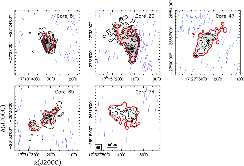
Figure 2.— IRAM 30-m MAMBO-II maps of the dust continuum emission at 1.2 mm toward five cores of the Pipe nebula. The grayscale levels for all the maps are 3 to 18 times 5.75 mJy beam^-1. The contour levels are 3 to 10 times $\sigma$ in steps of 1-$\sigma$, where 1-$\sigma$ is 4.0, 4.5, 4.9, 4.4, and 4.3 mJy beam^-1 for core 06, 20, 47, 65, and 74, respectively. The red thick contour marks the half maximum emission level of the source (Table 3). Black stars indicate the C¹⁸O pointing center reported by Muench et al. (2007). Black filled circles indicate the position where line observations have been performed, if different from the Muench et al. (2007) position, closer to the dust continuum emission maximum which falls into the beam area. The blue vectors depict the polarization vectors found by Franco et al. (2010). In the bottom left corner of the bottom middle panel the convolved beam and the spatial scale for the maps are shown.

Table 3 1.2 mm continuum emission parameters.

	$\alpha$(J2000)$~{}^{a}$	$\delta$(J2000)$~{}^{a}$	$T_{\rm dust}$	rms	$S_{\nu}$	$I_{\nu}^{\textrm{\tiny{Peak}}}$	Diameter b	$N_{\rm H_{2}}$ c	$n_{\rm H_{2}}$ c	Mass c
Source	h m s	$\arcdeg$ $\arcmin$ $\arcsec$	(K)	(mJy beam-1)	(Jy)	(mJy beam-1)	(pc)	(1021cm-2)	(104cm-3)	($M_{\odot}$)
Core 06	17 10 31.8	$-$27 25 51.3	10.0d	4.0	0.58	42.6	0.051	16.18 d	15.44 d	0.88 d
Core 20	17 15 11.5	$-$27 34 47.9	15.2e	4.5	1.52	42.6	0.088	7.33	4.04	1.20
Core 47	17 27 24.3	$-$26 57 22.2	12.6e	4.9	0.73	28.5	0.093	4.17	2.18	0.76
Core 65	17 31 21.1	$-$26 30 42.8	10.0d	4.4	0.48	36.1	0.053	12.39 d	11.38 d	0.73 d
Core 74	17 32 35.3	$-$26 15 54.0	10.0d	4.3	0.40	21.4	0.097	3.11 d	1.56 d	0.61 d

^a Dust continuum emission peak.
^b Diameter of the circle with area equal to the source area satisfying $I_{\nu}$$>$$I_{\nu}^{\rm Peak}/2$
^c Assuming $\kappa_{\rm 250~{}GHz}$$=$0.0066 cm² g^-1 as a medium value between dust grains with thin and thick ice mantles (Ossenkopf & Henning, 1994). See Appendix 1 in Paper I for details on the calculation.
^d No kinetic temperature estimate, therefore we assumed 10 K based on the average temperatures of the other cores in the Pipe nebula (Rathborne et al., 2008).
^e Adopted to be equal to the kinetic temperature estimated from NH₃ (Rathborne et al., 2008).

3.1. Dust continuum emission

In Fig. 2 we present the MAMBO-II maps of the dust continuum emission at 1.2 mm toward the five new cores of the Pipe nebula, convolved to a 21.$\!{}^{\prime\prime}$5 Gaussian beam in order to improve the signal-to-noise ratio (SNR), and to smooth the appearance of the maps. Table 3 lists the peak position of the 1.2 mm emission after convolution, the dust temperature (Rathborne et al., 2008), the rms noise of the maps, the flux density and the value of the emission peak. Additionally, we also give the derived full width half maximum (FWHM) equivalent diameter, H₂ column density ($N_{\rm H_{2}}$), H₂ volume density ($n_{\rm H_{2}}$) density, and mass for each core (see Appendix A in Paper I for details). These parameters are derived from the emission within the 3-$\sigma$ level assuming $\kappa_{\rm 250~{}GHz}$$=$0.0066 cm² g^-1 as a medium value between dust grains with thin and thick ice mantles (Ossenkopf & Henning, 1994), and discussed in Section 4.

The flux density of the cores ranges between $\sim$0.40 and $\sim$1.52 Jy, while the peak value ranges between $\sim$21 and $\sim$43 mJy beam^-1. The maps of Fig. 2 show the different morphology of the five cores. Core 06, located in the most evolved B59 region, shows one of the weakest emission levels ($\sim$0.6 Jy) of the present sample. It is the most compact ($\sim$0.05 pc) and densest ($\sim$1.5$\times$10⁵ cm^-3) core of the five. It shows similar physical properties to core 14 (Paper I), also in the B59 region. The two cores located in the stem, 20 and 47, show a very diffuse nature with elliptical morphologies similar to the previously presented stem core 48. The three of them have similar physical properties in terms of size ($\sim$0.09 pc) and density ($\sim$3$\times$10⁴ cm^-3). The bowl cores, 65 and 74, do not show a defined morphology. Their sizes, densities and masses are very different. Core 65 is more compact and denser, while core 74 shows properties comparable to those of the stem cores. The morphology of the dust continuum emission for all the cores is in good agreement with that of previous extinction maps (Lombardi et al., 2006; Román-Zúñiga et al., 2009).

Table 4 Summary of detections and upper levels in K toward the Pipe nebula cores^a.

Molecular	Core
transitions	06	14	20	40	47	48	65	74	109
C3H2 (21,2–11,0)	$\surd$	$\surd$	0.22	$\surd$	$\surd$	0.07	0.06	0.17	$\surd$
C2H (1–0)	$\surd$	$\surd$	$\surd$	$\surd$	$\surd$	$\surd$	0.06	–	$\surd$
HCN (1–0)	$\surd$	0.21	$\surd$	$\surd$	$\surd~{}^{b}$	$\surd$	–	0.18	$\surd$
N2H+ (1–0)	$\surd$	$\surd$	0.08	$\surd$	$\surd$	0.07	0.06	0.11	$\surd$
C34S (2–1)	$\surd$	$\surd$	$\surd$	$\surd$	$\surd$	$\surd$	0.07	$\surd$	$\surd$
CH3OH (2–1)	$\surd$	$\surd$	$\surd$	$\surd$	$\surd$	$\surd$	$\surd$	$\surd$	$\surd$
CS (2–1)	$\surd$	$\surd$	$\surd$	$\surd$	$\surd~{}^{b}$	$\surd$	–	$\surd$	$\surd$
C18O (1–0)	$\surd$	$\surd~{}^{b}$	$\surd~{}^{b}$	–	$\surd~{}^{b}$	–	–	$\surd$	$\surd~{}^{b}$
13CO (1–0)	$\surd$	$\surd~{}^{b}$	$\surd~{}^{b}$	–	$\surd~{}^{b}$	–	–	$\surd$	$\surd~{}^{b}$
CN (1–0)	$\surd$	$\surd$	0.25	$\surd$	$\surd$	0.17	0.11	0.19	$\surd$
C34S (3–2)	0.10	$\surd$	$\surd$	–	0.06	0.16	0.08	0.24	$\surd$
CS (3–2)	$\surd$	$\surd$	$\surd$	$\surd$	$\surd$	$\surd$	$\surd$	$\surd$	$\surd$
N2D+ (2–1)	0.04	0.12	0.17	$\surd$	0.09	0.08	0.08	0.09	$\surd$
DCO+ (3–2)	$\surd$	1.71	2.33	0.61	–	0.76	–	0.50	$\surd$
C18O (2–1)	$\surd$	$\surd~{}^{b}$	$\surd~{}^{b}$	$\surd~{}^{b}$	$\surd~{}^{b}$	$\surd$	$\surd$	$\surd$	$\surd~{}^{b}$
13CO (2–1)	$\surd$	$\surd~{}^{b}$	$\surd~{}^{b}$	–	$\surd~{}^{b}$	–	–	$\surd$	$\surd~{}^{b}$
CN (2–1)	0.80	0.97	–	1.70	–	0.76	–	0.84	0.90
N2D+ (3–2)	1.00	1.01	1.27 b	0.93	–	1.94	–	1.32	0.91
H13CO+ (3–2)	1.29	1.52	1.94$~{}^{b}$	1.40	–	2.38	–	1.84	1.34

^a Paper I results are included. The transitions marked with – have not been observed. Those marked with $\surd$ have been detected toward the corresponding core. Otherwise, the 3$\sigma$ upper limit is shown. In the seventh column of Table 2, early- and late-time labels are listed for each molecule.
^b Observed toward the extinction peak.

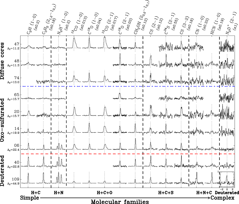
Figure 3.— Selected normalized molecular transitions toward the observed cores. The brightest transition is shown for the C₂H, CH₃OH, and HCN lines. The scale is shown in the bottom right spectrum. The normalized intensity axis ranges from -0.33 to 1, while the velocity axis spans 5 km s^-1 centered at the systemic velocity of the core. Rows: individual cores, labeled on the left-hand side of the figure, ordered by its $A_{\rm V}$ peak. Columns: molecular transition, ordered by molecular families, labeled on the top of the figure. The spectra have been divided by $[\mbox{$A_{\rm V}$}/100\,{\rm mag}]$ to mimic the abundance, where the $A_{\rm V}$ value is that at the respective core center (Román-Zúñiga et al., 2010) given below the core name. Each molecular transition has been multiplied by a factor, given below its name, to fit in a common scale.

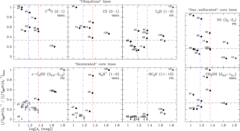
Figure 4.— Normalized integrated intensity ($A_{\rm V}$^-1 $\int T_{\rm MB}dv$) of selected molecular transitions divided by its maximum value as a function of the logarithm of the core $A_{\rm V}$ peak. Each panel shows the molecular transition in the top right corner. The backend is labeled below the molecular transition: VESPA panels present the nine cores of Paper I and present work, while FTS panels present the fourteen cores of Paper II. Filled circles represent the nine cores of Paper I and present work, stars represent the other six cores from Paper II (08, 12, 33, 56, 87, and 102), and arrows represent upper limits. Molecules have been split into the three categories defined in Paper II, labeled on the top of each group. The blue dot-dashed and red dashed vertical lines mark the transition from “diffuse” to “oxo-sulfurated”, and from “oxo-sulfurated” to “deuterated” cores, respectively. The horizontal dashed line marks a third of the peak value which helps to show the behavior change of the “oxo-sulfurated” and “deuterated” lines in our sample. The maximum values for each molecular transition are, in K km s^-1 mag^-1, 0.114, 0.036, and 0.030 for the ubiquitous C¹⁸O, CS, and C₂H, 0.059 and 0.025 for the “oxo-sulfurated” SO and CH₃OH, and 0.003, 0.010, and 0.019 for the “deuterated” c-C₃HD, N₂H⁺, and HC₃N, respectively.

3.2. Molecular survey of high density tracers

We present molecular line data observed toward the dust continuum emission peak or toward the C¹⁸O peak position reported by Muench et al. (2007, for more details see Fig. 2), defined as the core center and supposed to exhibit brighter emission from molecular transitions. As discussed in Paper I, the chemical properties derived toward the dust emission peak are representative of the chemistry at the core center. Our higher resolution dust emission maps show a peak offset with respect to the C¹⁸O for cores 20 and 47. For the former one, the offset is only $\sim$20″ while for the latter, more diffuse one, the offset is of $\sim$130″(see Section 4.4).

In Figs. 8–12, we show the spectra of the different molecular transitions observed toward the dust continuum emission peak of each core. Figures 8–9 show the molecular transitions with and without hyperfine components, respectively, for the five new cores. The new molecular transitions for the whole sample of nine cores are shown in Figs. 10–11, for those with hyperfine components, and Fig. 12, for those without hyperfine components. Table 4 summarizes the detections or the 3$\sigma$ upper limits of the non detections toward the whole sample of nine cores. We found that early-time molecules are broadly detected over the whole sample. Several of them were detected toward all the cores: CH₃OH (2–1), CS in the (2–1) and (3–2) transitions, and ¹³CO and C¹⁸O in the (1–0) and (2–1) transitions. On the other hand, only a few cores present emission of late-time molecules. The cores with $n_{\mathrm{H}_{2}}$$\sim$$>$10⁵ cm^-3 (06, 14, 40, and 109 but not 65) presented more detections than shallower cores and, indeed, were the only cores presenting N₂H⁺ emission. Tables 6–8 give the parameters of the detected lines. Regarding the line properties, the $\texttt{v}_{\rm LSR}$ measured for different species are generally consistent within 0.2 km s^-1. Intensities vary significantly over the sample: cores 06, 40 and 109 are generally bright while the rest of the sample shows fainter emission. “Bright” lines ($T_{\rm MB}$$>$0.2 K) are mostly very narrow (0.2$\sim$$<$$\Delta\texttt{v}$$\sim$$<$0.3 km s^-1), although transitions of CO and CS isotopologues can show broader profiles ($\Delta\texttt{v}$$\sim$$<$0.5 km s^-1 if “bright”). In some cases, this broadening can be explained in terms of a second velocity component generally merged with the main one (cores 06 and 20 in CS, and cores 06, 14, 47, 74, and 109 in ¹³CO).

In addition to the line parameters, we derived the molecular column densities for all the detected species (see Appendix B in Paper I for details) which are listed in Tables 9–10. For the transitions with detected hyperfine components (C₂H, HCN, N₂H⁺, CH₃OH, and CN), we derived the opacity using the hyperfine components fitting method (HFS) of the CLASS package. For the molecular transitions observed in more than one isotopologue, this is CS and C³⁴S in the (2–1) and (3–2) transitions, and ¹³CO and C¹⁸O in the (1–0) and (2–1) transitions, we derived numerically the opacity. Table 11 shows the H₂ column density of the cores for different angular resolutions. Tables 12–13 give the molecular abundances with respect to H₂.

Figure 3 shows the normalized intensities with respect to the core $A_{\rm V}$ peak of a selection of detected molecular transitions toward the sample of Paper I and the present work. Some of the lines were already presented in Paper II (except for core 74), although here are shown with a higher spectral resolution (e.g., the 3 mm C₂H, c-C₃H₂, and HCN line). The ¹³CO and C¹⁸O isotopologues can be considered as “ubiquitous” because they are present in all the observed cores (for cores 40, 48, and 65, the CO lines present intense emission but were observed toward a position that is offset from the core peak position). Their general trend is to decrease as density increases. The C³⁴S (2–1) line, which is optically thin, shows a similar trend as the main isotopologue (see Paper II), considered also as “ubiquitous”. The decrease in the normalized intensity in the CS lines is only apparent for the densest core 109. The CN normalized intensities are larger toward the densest cores, which suggests that CN is typically associated with the “deuterated” group. Late time species, such as N₂H⁺ and N₂D⁺, are only present in the densest cores and their emission tends to be brighter with increasing density, confirming that both species are typical of the “deuterated” group. These general results are in agreement with the observational classification of cores presented in Paper II, which is based on a wider molecular survey at 3 mm.

Finally, we defined the observational normalized integrated intensity (NII) as $\left(\int T_{\rm MB}dv\right)/A_{\rm V}$, to illustrate the different behavior of the molecular transitions that motivated the observational core classification proposed in Paper II. Figure 4 shows NII divided by its maximum value in the sample for selected molecular transitions typical of the three core groups: “diffuse”, “oxo-sulfurated”, and “deuterated”. “Ubiquitous” species are present in all the cores and their NII tends to decrease as the central density increases indicating possible depletion. “Oxo-sulfurated” species show low NII values except for a narrow range of densities ($A_{\rm V}$$\simeq$15-22 mag). CH₃OH (2_0,2–1_0,1) shows a similar behavior to the “oxo-sulfurated” species previously identified (e.g. SO, SO₂, and OCS; Paper II) but seems to peak at slightly larger densities ($A_{\rm V}$$\sim$20–23 mag). “Deuterated” species are only present toward the densest cores and their NII values increase with increasing density.

3.3. LTE status through hyperfine structure

We followed the procedure developed in Padovani et al. (2009) to study the departures from Local Thermodynamic Equilibrium (LTE) of two of the molecular transitions with hyperfine components, C₂H (1–0) and HCN (1–0), toward the Pipe nebula starless cores. By comparing ratios of integrated intensities between couples of the $i$-th and $j$-th component, $R_{ij}$, it is possible to check for opacity degree and LTE departures (Fig. 5). Under LTE and optically thin conditions, the relative weightings of C₂H (1–0) hyperfine components have the form 1:10:5:5:2:1, whereas for HCN (1–0) the relative intensities are 3:5:1. Figure 5 suggests that cores 40 and 109 are the most optically thick, in agreement with the determination of $\tau$ from the HFS fit in CLASS (Table 6), while the other cores are optically thin. Core 20 is a particular case because it shows $R_{54}$ and $R_{13}$ values in C₂H that cannot be reproduced with any value of $\tau$. This can be explained as the result of enhanced trapping due to an overpopulation of the $(N,J,F)=(0,1/2,1)$ level, where most $N=1-0$ transitions end (except for components 3 and 6; Padovani et al., 2009). This means that these results have to be thought in a qualitative way, since lines of very different intrinsic intensities experience different balance between trapping and collisions leading to excitation anomalies. The hyperfine components of HCN (1–0) do not obey the LTE weightings. For instance, as shown in Fig. 8, core 6 is affected by strong auto-absorption of the $F$=1–1 and $F$=2–1 components. Similarly, $F$=1–1 is stronger than $F$=2–1 in core 20. A more reliable determination of the HCN abundance would be given by the ¹³C (or ¹⁵N) isotopologue of HCN (Padovani et al., 2011). In general, cores seem to be close to LTE with those next to the optically thin limit showing the smallest LTE departures.

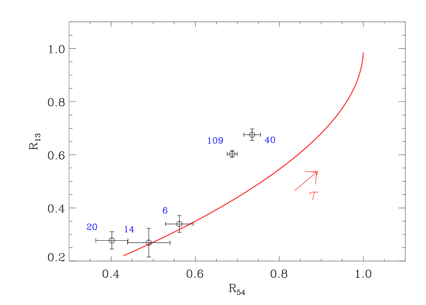
Figure 5.— Ratio of the integrated intensities of couples of components of C₂H (1–0) (upper panel, see Table 5 in Padovani et al., 2009 for labels) and HCN (1–0) (lower panel, see Table B.1 in Padovani et al., 2011 for labels). Empty circles: observational data labeled with the respective core number. Red solid line: one-slab LTE model, optical depth increases in the arrow direction (see Padovani et al., 2009 for details).

4. Discussion

4.1. Observational maps and physical structure of the cores

The extinction maps show that the cores in the Pipe nebula are surrounded by a diffuse medium (see Fig. 1 and Lombardi et al., 2006). Román-Zúñiga et al. (2012) show that the 1.2 mm continuum MAMBO-II maps underestimate the emission from the diffuse molecular component due to the reduction algorithms (see also Paper I). To study this effect, we compared, at the center of the nine cores, the $N_{\rm H_{2}}$ derived from the MAMBO-II maps (Table 11) with the $A_{\rm V}$ value from the extinction maps of Román-Zúñiga et al. (2009, 2010). We found a statistically significant correlation that can be expressed as

$$\mbox{$A_{\rm V}$}=(6.7\pm 1.5)+(1.27\pm 0.12)\times 10^{-21}N_{\rm H_{2}}.$$ (1)

The proportionality factor is compatible with the standard value (1.258$\times$10^-21 mag cm²; Wagenblast & Hartquist, 1989). However, the comparison evidences that the 1.2 mm maps underestimate the column density in average by an $A_{\rm V}$ of 6.7 mag, which is likely the contribution from the diffuse cloud material. As a consequence, the $A_{\rm V}$ peak values of the cores (from Román-Zúñiga et al., 2009, 2010) should be taken as upper limits of their column densities.

The statistics of this study have increased with the whole nine core sample. In Table 5 we show the main physical, chemical and polarimetric properties of the starless cores with respect to core 109 ordered by its decreasing $A_{\rm V}$ peak. Column and volume density, and total mass tend to decrease accordingly. On the contrary, the core diameter tends to increase. This suggests that denser cores are smaller and more compact, which is expected for structures in hydrostatic equilibrium such as Bonnor-Ebert spheres (Frau et al., in prep.). Under such assumption, gravitationally unstable cores ($n_{\rm H_{2}}$$\sim$$>$10⁵ cm^-3: Keto & Caselli, 2008) would slowly condense through a series of subsonic quasi-static equilibrium stages until the protostar is born and gravitational collapse starts, while gravitationally stable cores ($n_{\rm H_{2}}$$\sim$$<$10⁵ cm^-3) would achieve the equilibrium state and survive under modest perturbations (Keto & Field, 2005). The former group of cores would become denser with time while developing an increasingly richer chemistry, while the latter group would show a density-dependent chemistry (either in terms of active chemical paths and excitation effects) stable in time. This likely trends are supported by the clear correlation of the core chemistry with the visual extinction peak of the core and, therefore, its central density and structure (Section 4.5). Regarding the increasing mass with increasing central density, it seems unlikely that these young, diffuse cores efficiently accrete mass from the environment. This trend is most likely related to the initial conditions of formation of condensations in the low end of the cloud mass spectrum: an initially more massive condensation is more likely to form a dense structure.

Figure 6.— Relation of the core major axis orientation ($\theta_{\rm core}$) to different physical parameters. a: $\theta_{\rm core}$ against mean polarization angle ($\theta_{\rm Pol}$) of the corresponding observed field (Franco et al., 2010). b-d: $\theta_{\rm Pol}$-$\theta_{\rm core}$ as a function of core $A_{\rm V}$ peak (Román-Zúñiga et al., 2009, 2010), polarization fraction ($p_{\%}$) and polarization angle dispersion ($\delta$P.A.), respectively.

4.2. Relationship between the large scale magnetic field and the elongation of the cores

The Pipe nebula cores are embedded in a sub-Alvénic molecular cloud that is threaded with a strikingly uniform magnetic field (Alves et al., 2008; Franco et al., 2010). Thus, it is possible that the core formation is related to the magnetic field and its direction is related to the core elongations. Figure 2 of both Paper I and the present work show that the polarization vectors calculated from optical data cannot trace the densest part of the cores although the vectors lie very close to the core boundaries (up to $A_{\rm V}$$\sim$5 mag). To derive the orientation of the core major axis, we computed the integrated flux within the FWHM contour for a series of parallel strips (11″ wide), with position angles in the -90^∘ to 90^∘ range. The major axis is oriented in the direction with the largest integrated flux on the fewest strips. We found no correlation between the orientation of the major axis of the core, $\theta_{\rm core}$, and the diffuse gas mean magnetic field direction around the cores ($\theta_{\rm Pol}$, see Fig. 6$a$). To investigate more subtle effects, we compared for each core the difference between polarization position angle and the major axis orientation ($\theta_{\rm Pol}$-$\theta_{\rm core}$) with respect to the $A_{\rm V}$ peak, the polarization fraction ($p_{\%}$) and polarization angle dispersion ($\delta$P.A.) estimated in a region of few arc-minutes around the cores (Franco et al., 2010). The results of these comparisons are shown in panels $b$, $c$ and $d$ of Fig. 6, respectively. Again, it seems that there are no clear correlations between these quantities.

These results suggest that the well-ordered, large scale magnetic field that may have driven the gas to form the $\sim$15 pc long filamentary cloud, and shows uniform properties for the diffuse gas at scales ranging $\sim$$<$0.01 pc up to several pc (Franco et al., 2010), has little effect in shaping the morphology of the denser $\sim$0.1 pc cores. At intermediate scales, Peretto et al. (2012) suggest that a large scale compressive flow has contributed to the formation of a rich, organized network of filamentary structures within the cloud, $\sim$0.1 pc wide and up to a few pc long, which tend to align either parallel or perpendicular to the magnetic field. If this is the case, then, rather than ambipolar diffusion, other mechanisms such as a compressive flow should play a major role in the formation of the Pipe nebula cores. However, as pointed out by Lada et al. (2008), the cores in the Pipe nebula evolve on acoustic, and thus, slow timescales ($\sim$$10^{6}$ yr), allowing ambipolar diffusion to have significant effects. Furthermore, the lack of spherical symmetry demands an anisotropic active force. Projection effects, together with the small statistical sample, require a deeper study of the magnetic field properties. In order to extract firm conclusions and disentangle the nature of the formation of the Pipe nebula cores, the magnetic field toward the dense gas needs to be studied.

Table 5 Pipe nebula Core General Properties with Respect to Core 109^a

Source	Diameter	Mass	$N_{\rm H_{2}}$	$n_{\rm H_{2}}$	$p_{\%}^{b}$	$\delta$P.A.b	X(C18O)	X(CS)	X(C2H)	X(C3H2)	X(CH3OH)	X(CN)	X(N2H+)
	(pc)	($M_{\odot}$)	(1021cm-2)	(104cm-3)	(%)	(o)	(10-11)	(10-11)	(10-11)	(10-11)	(10-11)	(10-11)	(10-11)
Core 109	0.063	4.00	47.60	36.57	11.0	3.9	1324.6	40.2	34.1	52.8	44.3	8.7	2.2
Relative Values (%)
Core 109	100	100	100	100	100	100	100	100	100	100	100	100	100
Core 40	165	63	23	14	42	222	517	168	335	52	272	480	208
Core 06	86	23	32	38	22	249	323	315	125	12	609	105	243
Core 14	113	35	28	25	18	404	1051	752	89	7	368	121	44
Core 20	141	28	14	10	29	160	752	576	295	$<$ 7	186	$<$ 36	$<$ 37
Core 65	105	26	23	22	126	80	608	–	$<$ 3	$<$ 2	99	$<$ 13	$<$ 20
Core 74	154	16	7	4	140	84	303	435	$<$ 3	$<$ 5	96	$<$ 27	$<$ 36
Core 48	202	52	13	6	18	838	553	539	162	$<$ 2	72	$<$ 20	$<$ 25
Core 47	146	19	9	6	56	101	521	–	298	13	204	511	117

^a Molecules are ordered from earlier to later synthesization. Cores are ordered in three groups following Paper II.
^b Franco et al. (2010)

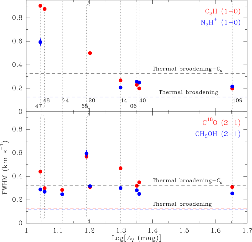
Figure 7.— Top panel: line width of the C₂H (1–0) and N₂H⁺ (1–0) lines, colored in red and blue, respectively, as a function of the logarithm of the core $A_{\rm V}$ peak. Bottom panel: Same as top panel but for the C¹⁸O (2–1) and CH₃OH (2–1) lines, colored in red and blue, respectively. Colored dashed horizontal lines show the corresponding thermal line width for each molecule for a temperature of 10 K. Black dashed horizontal lines show the average thermal line width plus the sound speed ($C_{s}$) at 10 K. Vertical dotted lines mark the $A_{\rm V}$ peak of each core, which in the case of similar values (cores 47 and 48, and 20 and 65) have been slightly displaced.

4.3. Velocity dispersion analysis

Figure 7 shows the FWHM line width of four selected molecular transitions at 3 mm as a function of the core $A_{\rm V}$ peak. Whereas the C¹⁸O and CH₃OH lines show an almost constant line width of 0.3–0.4 km s^-1 for most cores (except core 65), the C₂H and N₂H⁺ lines have a lower line width, 0.20–0.25 km s^-1, except for the cores with lower visual extinction (47, 48 and 20). The values of the C¹⁸O line are in agreement with those found by Muench et al. (2007) with lower angular resolution. In most cases, the line widths are only 2–3 times the thermal broadening at 10 K. These line widths imply a subsonic non-thermal velocity dispersion, $\sigma_{\rm NT}$, of 0.06–0.09 km s^-1 for the N₂H⁺ and C₂H lines, respectively, and of 0.12–0.16 km s^-1 for the C¹⁸O and CH₃OH lines, respectively. Therefore, the thermal pressure dominates the internal pressure of the cores, which is a general characteristic of the Pipe nebula (Lada et al., 2008). For the higher density cores ($A_{\rm V}$$>17$ mag), smaller $\sigma_{\rm NT}$ for the N₂H⁺ and C₂H lines with respect to C¹⁸O and CH₃OH lines suggests that the former transitions are tracing the inner regions of the core. However, cores 47 and 48 present a peculiar reverse case in the line width properties, i.e., the C₂H and N₂H⁺ lines are significantly wider and clearly supersonic. This is compatible with the plausible scenario of core 47 (and probably core 48) being a failed core in re-expansion (Frau et al., 2012), on which the centrally synthesized and initially narrow N₂H⁺ and C₂H (1–0) lines are now part of the disrupted gas. But it is puzzling that the C¹⁸O and CH₃OH lines are still narrow and subsonic, unless they trace a part of core that still remains unperturbed. A complete mapping of these cores is needed to reveal their striking nature.

4.4. Discussion on the individual cores

Core 06, located in the western part of B59, is a compact and dense core. The dust continuum emission is similar to the extinction maps (Román-Zúñiga et al., 2009). The core shows a rich chemistry with bright detections of all the early-time and some late-time molecules. The core has the brightest emission and highest abundance of CH₃OH of the sample, as well as the highest N₂H⁺ abundance. Unlike core 109, it has a high CS abundance suggesting that it has not been depleted yet. All these features suggest that core 06 is in the “oxo-sulfurated” group close to the “deuterated” cores.

Core 20, located in the stem, shows in the 1.2 mm map two components: a compact and bright one surrounded by a second one, extended and diffuse. Most of the early-time molecules were detected, and thus, this core seems to be very young chemically showing abundances in CS and CH₃OH among the highest. Normalized intensities are in general quite large for its density (Fig. 3), and it has a very large SO normalized integrated intensity as core 47 (Fig. 4). These signposts suggest that core 20 belongs to the “oxo-sulfurated” group.

Core 47, located between the stem and the bowl, has extended and diffuse dust emission. It shows a fairly uniform and weak emission all over the $A_{\rm V}$ and MAMBO-II maps. This can explain the peak position difference of $\sim$130″ between the dust emission map and the position taken by Muench et al. (2007) for the line observations. It shows weak line emission, only in early-time molecules. It is the second least dense core of the sample ($\sim$2$\times$10⁴ cm^-3), yet the molecular abundances tend to be among the highest. Rathborne et al. (2008) report a clear detection of NH₃ (1,1) and hints of emission in the (2,2) transition. Figure 8 shows a marginal detection at 3$\sigma$ level of the N₂H⁺ (1–0) brightest hyperfine component. The high molecular abundances and the emission of certain molecular line tracers of the “oxo-sulfurated” group, together with its diffuse morphology and low density typical of the “diffuse” cores, suggest that core 47 may be an evolved failed core now in re-expansion as already suggested in Paper II. The relatively broad lines in some of the species (see Section 4.3) support this scenario.

Core 65, located in the bowl, is the central core of a group of three (see Fig. 2). Its density is in the limit between those of the “diffuse” and “oxo-sulfurated” cores. It has a very poor chemistry with only “ubiquitous” early-time molecules detected (CO, CS, and CH₃OH) with abundances among the lowest of the sample. The line widths, $\sim$0.6 km s^-1, appear to be larger than those of the other cores.

Finally, core 74, located in the bowl, is extended and diffuse similarly to core 47. It also shows a very poor chemistry with only “ubiquitous” early-time molecules detected (CO, CS, and CH₃OH).

It is useful to review the data from Rathborne et al. (2008). The late-time molecule NH₃ in the (1,1) transition is detected in cores 06, 20, 47, and marginally in 65. These cores belong to the “oxo-sulfurated” group, which suggests that NH₃ is formed in this phase. CCS is considered an early-time molecule with a lifetime of $\sim$$<$3$\times$10⁴ yr (de Gregorio-Monsalvo et al., 2006). It is only marginally detected toward core 06, therefore suggesting that it might be very young. Core 74 does not show any emission, in agreement with the poor chemistry detected in our 3 mm surveys. These results also suggest that the five cores are in a very early stage of evolution.

4.5. Qualitative chemistry discussion

The molecular transitions from Paper I and this work increase the number of typical lines of the core categories established in Paper II. Four of the five cores have lower densities than the initial subsample (except for core 48, Table 11), and thus, we are now including in the analysis shallower cores that might be more affected by the external radiation field and that show a younger chemistry (although the timescale to form the core may influence this evolution: Tafalla et al., 2004; Crapsi et al., 2005).

We found a complex chemical scenario toward the Pipe nebula cores. However, as pointed out in Paper II, it seems that there is a chemical trend with density in the form of three differentiated core chemical groups. We remind that the $A_{\rm V}$ values should be interpreted as upper limits for the column density of the cores (Section 4.1), and that the column densities derived from the dust emission maps show larger differences than the $A_{\rm V}$ values. These facts translate to larger abundance differences among the cores as compared to the normalized intensity differences. The molecular trends, however, are compatible. We will base our analysis in the combination of the results obtained via the normalized intensities and normalized integrated intensities (Figs. 3 and 4), and of the molecular abundances with respect to the H₂ (Table 5), to which we will refer generically as abundances. C¹⁸O and CS lines appear to be “ubiquitous”, as they are detected in all the cores. Their abundances decrease with column density due to, probably, an increasingly efficient depletion for both species (and isotopologues) as density grows. The variation of the CN abundance among the cores has increased with respect to Paper I (up to a factor of $\sim$33 in abundance: Table 13), due to the addition of more diffuse cores. The lower limits are indeed very low, and thus, we are now exploring even younger chemical stages of these starless cores. All these features suggest that CN (1–0) is a transition typical of the “deuterated” group. A nitrogen- (N₂H⁺) and a deuterium-bearing (c-C₃HD) species, and a carbon chain molecule (HC₃N) are shown in Fig. 4. These late-time molecules, present toward the densest objects, are not detected in low density cores. They are only present after achieving a density threshold, and exhibit increasing abundances as density grows. These transitions seem to be typical of the “deuterated” cores, which is consistent with the detection of NH₂D (1_1,1–1_0,1) toward this core group in Paper II.

In order to analyze possible excitation effects in the detected emission we consider now the N₂H⁺ (1–0) transition whose critical density ($n_{\rm cr}$=2$\times$10⁵ cm^-3: Ungerechts et al., 1997) lies within the density range of the studied cores. The different excitation conditions could explain the differences between the densest core (109) and the least dense cores with no detections (20, 48, and 74), having the latter ones $n_{\rm H_{2}}$ (toward the central beam derived from Table 11) close to $n_{\rm cr}$. Indeed, we used RADEX (van der Tak et al., 2007) assuming as representative values $X\left({\rm N_{2}H^{+}}\right)$=2$\times$10^-11, $T$=10 K, and $\sigma$=0.25 km s^-1, and found that a volume density increase from 4$\times$10⁵ cm^-3 to 1.4$\times$10⁶ cm^-3 (average values toward the central beam of cores 6 and 109, respectively) produces a difference in $T_{\rm MB}$ of a factor of 3 while the observed peaks are one order of magnitude apart, suggesting real differences in the abundances rather than excitation effects. The observational classification proposed, although based on groups of molecules and peak $A_{\rm V}$ values, is sensitive to these effects as the $A_{\rm V}$ values are related to those of $n_{\rm H_{2}}$. However, a more careful study should be done when studying individual molecules to be compared to chemical modelling results.

CH₃OH deserves a special mention. This molecule is clearly detected in the gas phase toward all the observed cores in the (2_0,2–1_0,1) (shown normalized in Fig. 3) and (2_1,2–1_1,1) transitions (Fig. 10). It shows a behavior similar to that of the “oxo-sulfurated” species but peaking at slightly larger densities. Thus, this species is likely to peak in the transition from the “oxo-sulfurated” core chemistry to the typical dense core chemistry found toward the “deuterated” cores, suggesting that CH₃OH could be actually an early-time molecule. It is expected to be formed efficiently in grain surfaces, with abundances for the gas phase of $\sim$10^-9 at most (Cuppen et al., 2009; Garrod & Pauly, 2011), very close to the observational abundances derived ($\sim$3$\times$10^-10–$\sim$3$\times$10^-9: Table 12). Abundances for the gas phase of 6$\times$10^-10, comparable to the lowest values for the Pipe nebula cores, have been derived in the literature through modeling of more evolved low-mass cores (Tafalla et al., 2006). However, the higher densities and comparable temperatures product of this modeling with respect to the Pipe nebula core values suggest that other mechanisms are needed to explain the high gas phase CH₃OH abundances found here. In addition, the abundances in the Pipe nebula cores seem to correlate with their location in the cloud, being larger in the B59 region and decreasing as going toward the bowl. This fact could be explained by the slightly higher temperatures reported toward the B59 region (Rathborne et al., 2008), which could enhance evaporation from grains.

In summary, our high spectral resolution dataset shows the existence of a clear chemical differentiation toward the Pipe nebula cores. The chemical signatures agree with the results of previous Papers I and II. Chemistry seems to become more rich and complex as cores grow denser therefore suggesting an evolutionary gradient among the sample. The tentative correlation found in Paper I between magnetic field and chemical evolutionary stage of the cores is less clear with the whole nine core sample.

5. Summary and conclusions

We carried out observations of continuum and line emission toward five starless cores, located on the three different regions of the Pipe nebula, and combined them with the observations of the four additional cores of Paper I to extend the dataset to nine cores. We studied the physical and chemical properties of the cores, and their correlation following Paper II. We also studied the correlation with the magnetic field properties of the surrounding diffuse gas following Paper I.

1. The Pipe nebula starless cores show very different morphologies. The complete sample of nine cores contains dense and compact cores (6, 65, and 109; $n_{\rm H_{2}}$$\sim$$>$10⁵ cm^-3), diffuse and elliptical/irregular ones (20, 40, 47, 48, and 74; $n_{\rm H_{2}}$$\sim$$<$5$\times$10⁴ cm^-3), and a filament containing the relatively dense core 14 ($n_{\rm H_{2}}$$\sim$9$\times$10⁴ cm^-3). The average properties of the nine cores of the sample are diameter of $\sim$0.08 pc ($\sim$16,800 AU), density of $\sim$10⁵ cm^-3, and mass of $\sim$1.7 $M_{\odot}$. These values are very close to (but less dense than) those reported by Ward-Thompson et al. (1999) for a set of very young dense cores and, therefore, typical of even earlier stages of evolution.

2. MAMBO-II maps are in a general good morphological agreement with previous extinction maps (Lombardi et al., 2006). By comparing the $A_{\rm V}$ peak values of the nine cores from deeper NICER maps (Román-Zúñiga et al., 2009, 2010), we derived a proportionality factor $A_{\rm V}$/$N_{\rm H_{2}}$=(1.27$\pm$0.12)$\times$10^-21 mag cm², compatible with the standard value (1.258$\times$10^-21 mag cm²; Wagenblast & Hartquist, 1989). In addition, we found that dust continuum maps underestimate the column density by an $A_{\rm V}$ of $\sim$6.7 mag that may be arising from the diffuse material of the cloud.

3. The orientation of the cores is not correlated with the surrounding diffuse gas magnetic field direction, which suggests that large scale magnetic fields are not important in shaping the cores. On the other hand, the lack of spherical symmetry demands an important anisotropic force, and projection effects might be important. A deeper study of the magnetic field of the dense gas is needed.

4. The analysis of the line widths reports two behaviors depending on the molecular transition: (i) a roughly constant value of subsonic turbulent broadening for all the cores (e.g. C¹⁸O (1–0) and CH₃OH (2–1), see also Lada et al., 2008) and (ii) a roughly constant slightly narrower broadening for cores with $A_{\rm V}$$\sim$$>$20 mag and supersonic turbulent broadenings otherwise (e.g. C₂H (1–0) and N₂H⁺ (1–0)).

5. We observed a set of early- and late-time molecular transitions toward the cores and derived their column densities and abundances. The high spectral resolution molecular normalized line data is in agreement with the lower spectral resolution data presented in Paper II. The nine starless cores are all very chemically young but show different chemical properties. “Diffuse” cores ($A_{\rm V}$$\sim$$<$15 mag: 48 and 74) show emission only in “ubiquitous” lines typical of the parental cloud chemistry (e.g. CO, CS, CH₃OH). The denser “deuterated” cores ($A_{\rm V}$$\sim$$>$22 mag: 40 and 109) show weaker abundances for “ubiquitous” lines and present emission in nitrogen- (N₂H⁺) and deuterium-bearing (c-C₃HD) molecules, and in some carbon chain molecules (HC₃N), signposts of a prototypical dense core chemistry. “Oxo-sulfurated” cores ($A_{\rm V}$$\simeq$15–22 mag: 6, 14, 20, and 65) are in a chemical transitional stage between cloud and dense core chemistry. They are characterized by presenting large abundances of CH₃OH and oxo-sulfurated molecules (e.g. SO and SO₂) that disappear at higher densities, and they still present significant emission in the “ubiquitous” lines. CH₃OH was detected toward the nine cores of the complete sample with abundances of $\sim$10^-9, close to the maximum value expected for gas-phase chemistry.

6. Core 47 presents high abundance of CH₃OH and N₂H⁺, in spite of being the core with the lowest H₂ column density, and broad line width in some species (C₂H and N₂H⁺). All this is in agreement with the hypothesis given in Paper II, which suggests that Core 47 could be a failed core.

7. The chemical evolutionary stage is not correlated with the core location in the Pipe nebula, but it is correlated with the physical properties of the cores (density and size). Thus, the chemically richer cores are the denser ones. The tentative correlation between magnetic field and chemical properties found for the initial subsample of four cores is less clear with the current sample.

The Pipe nebula is confirmed as an excellent laboratory for studying the very early stages of star formation. The nine cores studied show different morphologies and different chemical and magnetic properties. Physical and chemical properties seem to be related, although important differences arise, which evidence the complex interplay among thermal, magnetic, and turbulent energies at core scales. Therefore, a larger statistics is needed to better understand and characterize the Pipe nebula starless core evolution. In addition, other young clouds with low-mass dense cores, such as the more evolved star-forming Taurus cloud, should be studied in a similar way to prove the presented results as a general trend or, on the contrary, a particular case for a filamentary magnetized cloud.

Appendix A On line material: Tables and Figures

Table 6 Line parameters^a.

Molecular		$T_{\rm MB}$ b		$A\times\tau$ c		$\int T_{\rm MB}\mbox{d}\texttt{v}$ b		$\texttt{v}_{\rm LSR}$		$\Delta\texttt{v}_{\rm LSR}$
transition	Source	(K)		(K)		(K  km s-1)		(km s-1)		(km s-1)		$\tau$ d		Profilee
C3H2 (21,2–11,0)	Core 06	0.	502(24)	–		0.	140(5)	3.	574(4)	0.	262(11)	–		G
	Core 14	0.	37(6)	–		0.	086(11)	3.	502(14)	0.	22(3)	–		G
	Core 40	1.	19(5)	–		0.	347(9)	3.	420(4)	0.	273(9)	–		G
	Core 47	0.	079(22)	–		0.	071(8)	3.	11(5)	0.	85(8)	–		G
	Core 109	2.	74(6)	–		0.	799(13)	5.	8340(20)	0.	274(5)	–		G
C2H (1–0)	Core 06	–		0.	389(7)	–		3.	6200(8)	0.	2300(19)	0.	655(21)	G
	Core 14	–		0.	1650(24)	–		3.	5800(13)	0.	268(3)	0.	450(9)	G
	Core 20	–		0.	1140(25)	–		3.	7900(19)	0.	500(6)	0.	193(16)	G
	Core 40	–		2.	03(3)	–		3.	4700(4)	0.	1990(8)	2.	58(4)	G
	Core 47	–		0.	0345(5)	–		3.	140(7)	0.	903(15)	0.	1000(4)	G
	Core 48	–		0.	0255(5)	–		3.	630(9)	0.	876(21)	0.	1000(16)	G
	Core 109	–		2.	280(9)	–		5.	89000(13)	0.	1980(3)	1.	530(8)	G
CH3OH (20,2–10,1)	Core 06	1.	841(15)	–		0.	55(3)	3.	512(7)	0.	281(15)	–		G
	Core 14	1.	30(3)	–		0.	416(21)	3.	519(7)	0.	300(17)	–		G
	Core 20	0.	43(3)	–		0.	145(10)	3.	653(10)	0.	316(24)	–		G
	Core 40	1.	230(15)	–		0.	327(16)	3.	375(6)	0.	250(14)	–		G
	Core 47	0.	45(3)	–		0.	138(10)	2.	845(10)	0.	288(24)	–		G
	Core 48	0.	199(25)	–		0.	057(6)	3.	652(13)	0.	27(3)	–		G
	Core 65	0.	15(3)	–		0.	098(9)	5.	04(3)	0.	59(6)	–		G
	Core 74	0.	257(21)	–		0.	068(5)	4.	201(9)	0.	247(22)	–		G
	Core 109	1.	27(3)	–		0.	343(18)	5.	778(6)	0.	254(15)	–		G
CH3OH (2-1,2–1-1,1)	Core 06	1.	432(15)	–		0.	417(4)	3.	5055(10)	0.	273(3)	–		G
	Core 14	1.	04(3)	–		0.	306(6)	3.	508(3)	0.	276(7)	–		G
	Core 20	0.	35(3)	–		0.	094(6)	3.	672(8)	0.	250(20)	–		G
	Core 40	0.	998(15)	–		0.	252(3)	3.	3705(10)	0.	237(3)	–		G
	Core 47	0.	33(3)	–		0.	119(7)	2.	847(10)	0.	344(22)	–		G
	Core 48	0.	134(25)	–		0.	047(5)	3.	641(19)	0.	33(5)	–		G
	Core 65	0.	12(3)	–		0.	063(7)	4.	98(3)	0.	48(6)	–		G
	Core 74	0.	212(21)	–		0.	059(4)	4.	201(9)	0.	261(20)	–		G
	Core 109	1.	03(3)	–		0.	263(5)	5.	7705(20)	0.	240(6)	–		G
CN (1–0)	Core 06	–		0.	17(5)	–		3.	640(15)	0.	30(3)	1.	2(4)	G
	Core 14	–		0.	051(9)	–		3.	64(8)	0.	81(15)	0.	1(7)	G
	Core 40	–		0.	65(22)	–		3.	430(21)	0.	36(5)	3.	9(1.3)	G
	Core 47	–		0.	10(4)	–		2.	98(5)	0.	80(13)	0.	9(5)	G
	Core 109	–		1.	41(22)	–		5.	930(5)	0.	162(11)	1.	13(23)	G
		–		2.	3(1.3)	–		5.	670(7)	0.	101(16)	4.	(3)
HCN (1–0)	Core 06	–		0.	025(6)	–		3.	56(3)	0.	76(8)	0.	11(5)	G
	Core 20	–		0.	059(16)	–		3.	58(3)	0.	68(7)	0.	24(8)	G
	Core 40	–		1.	55(11)	–		3.	410(16)	0.	334(22)	6.	0(5)	NS
	Core 47	–		0.	051(13)	–		2.	93(3)	0.	72(7)	0.	27(8)	G
	Core 48	–		0.	33(10)	–		3.	54(5)	0.	90(11)	2.	4(1.2)	G
	Core 109	–		2.	53(3)	–		5.	93(7)	0.	16(22)	0.	25(10)	NS
		–		6.	10(3)	–		5.	72(7)	0.	25(22)	10.	20(10)
N2H+ (1–0)	Core 06	–		0.	119(5)	–		3.	5000(16)	0.	257(4)	0.	10(10)	G
	Core 14	–		0.	0341(16)	–		3.	500(5)	0.	206(10)	0.	10(9)	G
	Core 40	–		0.	219(12)	–		3.	4000(19)	0.	249(5)	0.	171(25)	G
	Core 47	–		0.	0100(9)	–		3.	00(4)	0.	59(6)	0.	10(3)	G
	Core 109	–		0.	904(14)	–		5.	8000(5)	0.	2150(11)	0.	467(11)	G
N2D+ (2–1)f	Core 40	0.	084(20)	–		0.	019(3)	3.	280(15)	0.	21(3)	–		G
	Core 109	0.	31(4)	–		0.	109(7)	5.	673(11)	0.	331(22)	–		G
DCO+ (3–2)	Core 06	0.	44(13)	–		0.	22(3)	3.	58(3)	0.	48(11)	–		G
	Core 109	0.	70(11)	–		0.	151(18)	5.	828(13)	0.	202(21)	–		G

^a Line parameters of the detected lines. Multiple velocity components are shown if present. For the molecular transitions with no hyperfine components, the parameters for the transitions labeled as G (last column) have been derived from a Gaussian fit while line parameters of NS and SA profiles have been derived from the intensity peak ($T_{\rm MB}$), and zero (integrated intensity), first (line velocity) and second (line width) order moments of the emission. For the molecular transitions with hyperfine components, the parameters have been derived using the hyperfine component fitting method of the CLASS package. The value in parenthesis shows the uncertainty of the last digit/s. If the two first significative digits of the error are smaller than 25, two digits are given to better constrain it.
^b Only for molecular transitions with no hyperfine components.
^c Only for molecular transitions with hyperfine components.
^d Derived from a CLASS hyperfine fit for molecular transitions with hyperfine components. Derived numerically for CS, C³⁴S, ¹³CO, and C¹⁸O using Eq. 1 from Paper I. A value of 0.1 is assumed when no measurement is available.
^e G: Gaussian profile. NS: Non-symmetric profile. SA: Self-absorption profile.
^f Only the main component is detected.

Table 7 Line parameters^a (Continuation).

Molecular		$T_{\rm MB}$ b		$A\times\tau$ c	$\int T_{\rm MB}\mbox{d}\texttt{v}$ b		$\texttt{v}_{\rm LSR}$		$\Delta\texttt{v}_{\rm LSR}$
transition	Source	(K)		(K)	(K  km s-1)		(km s-1)		(km s-1)		$\tau$ d		Profilee
C34S (2–1)	Core 06	0.	207(16)	–	0.	055(3)	3.	551(7)	0.	247(15)	0.	182(18)	G
	Core 14	0.	267(25)	–	0.	068(5)	3.	545(8)	0.	241(20)	0.	48(5)	G
	Core 20	0.	18(4)	–	0.	057(7)	3.	718(19)	0.	30(4)	0.	154(15)	G
	Core 40	0.	268(16)	–	0.	069(3)	3.	381(5)	0.	241(13)	0.	140(14)	G
	Core 47	0.	07(4)	–	0.	042(10)	3.	00(7)	0.	53(13)	0.	036(4)	G
	Core 48	0.	187(23)	–	0.	041(4)	3.	729(11)	0.	20(3)	0.	26(3)	G
	Core 74	0.	137(21)	–	0.	027(3)	4.	236(12)	0.	186(23)	0.	228(23)	G
	Core 109	0.	34(3)	–	0.	083(5)	5.	825(7)	0.	233(17)	0.	185(18)	G
CS (2–1)	Core 06	1.	20(6)	–	0.	30(3)	3.	429(11)	0.	237(21)	4.	1(4)	G
		0.	56(6)	–	0.	14(3)	3.	698(22)	0.	23(5)	–
	Core 14	0.	69(10)	–	0.	41(3)	3.	439(21)	0.	45(4)	10.	7(1.1)	SA
	Core 20	1.	18(9)	–	0.	34(4)	3.	469(12)	0.	27(3)	3.	5(3)	G
		1.	10(9)	–	0.	35(4)	3.	820(14)	0.	30(3)	–
	Core 40	1.	94(7)	–	0.	560(17)	3.	369(4)	0.	415(14)	3.	1(3)	NS
	Core 47	1.	16(9)	–	0.	609(24)	2.	817(10)	0.	495(23)	0.	81(8)	G
	Core 48	0.	79(7)	–	0.	402(18)	3.	684(11)	0.	477(22)	6.	0(6)	SA
	Core 74	0.	66(8)	–	0.	268(17)	4.	245(13)	0.	38(3)	5.	1(5)	G
	Core 109	1.	93(8)	–	0.	743(17)	5.	836(4)	0.	361(9)	4.	2(4)	G
C34S (3–2)	Core 14	0.	12(3)	–	0.	034(4)	3.	488(17)	0.	27(4)	1.	70(17)	G
	Core 20	0.	15(5)	–	0.	064(11)	3.	59(3)	0.	40(8)	0.	25(3)	G
	Core 109	0.	18(6)	–	0.	064(8)	5.	82(3)	0.	340(00)	0.	189(19)	G
CS (3–2)	Core 06	0.	68(6)	–	0.	220(10)	3.	480(7)	0.	303(15)	–		G
	Core 14	0.	14(4)	–	0.	072(7)	3.	59(3)	0.	48(4)	38.	(4)	G
	Core 20	0.	67(6)	–	0.	179(8)	3.	502(8)	0.	2500(00)	5.	7(6)	G
		0.	65(6)	–	0.	173(8)	3.	797(9)	0.	2500(00)	–
	Core 40	1.	09(9)	–	0.	270(13)	3.	414(6)	0.	234(15)	–		G
	Core 47	0.	35(6)	–	0.	148(11)	2.	896(15)	0.	39(3)	–		G
	Core 48	0.	28(5)	–	0.	122(10)	3.	772(17)	0.	41(4)	–		G
	Core 65	0.	16(4)	–	0.	124(11)	5.	07(4)	0.	73(9)	–		G
	Core 74	0.	34(5)	–	0.	100(8)	4.	200(11)	0.	277(20)	–		G
	Core 109	1.	01(8)	–	0.	366(14)	5.	810(7)	0.	339(15)	4.	2(4)	G

Footnotes ^a to ^e as in Table 6.

Table 8 Line parameters^a (Continuation).

Molecular		$T_{\rm MB}$ b		$A\times\tau$ c	$\int T_{\rm MB}\mbox{d}\texttt{v}$ b		$\texttt{v}_{\rm LSR}$		$\Delta\texttt{v}_{\rm LSR}$
transition	Source	(K)		(K)	(K  km s-1)		(km s-1)		(km s-1)		$\tau$ d		Profilee
C18O (1–0)	Core 06	2.	61(6)	–	1.	137(13)	3.	5180(20)	0.	409(6)	0.	33(3)	G
	Core 14	4.	10(6)	–	1.	875(13)	3.	4890(10)	0.	430(4)	0.	84(8)	G
	Core 20	2.	97(6)	–	0.	798(10)	3.	6600(20)	0.	253(4)	0.	31(3)	G
	Core 47	2.	51(6)	–	1.	116(14)	2.	791(3)	0.	417(6)	0.	50(5)	G
	Core 74	2.	51(5)	–	0.	961(10)	4.	1920(20)	0.	360(5)	0.	59(6)	G
	Core 109	2.	42(5)	–	0.	991(11)	5.	7640(20)	0.	384(5)	0.	51(5)	G
13CO (1–0)	Core 06	7.	78(6)	–	4.	98(11)	3.	536(5)	0.	601(6)	1.	83(18)	G
		1.	96(6)	–	1.	44(11)	4.	133(24)	0.	69(3)	–
	Core 14	7.	13(6)	–	4.	407(18)	3.	4280(10)	0.	581(4)	4.	7(5)	G
		4.	13(6)	–	2.	639(4)	3.	8680(20)	0.	600(6)	–
	Core 20	9.	12(6)	–	5.	903(16)	3.	7060(10)	0.	6080(20)	1.	71(17)	G
	Core 47	5.	99(5)	–	3.	647(12)	2.	7550(10)	0.	5720(20)	2.	8(3)	G
		4.	27(5)	–	3.	912(14)	3.	2300(20)	0.	862(4)	–
	Core 74	5.	41(5)	–	3.	598(21)	4.	2320(20)	0.	625(4)	3.	3(3)	G
		2.	15(5)	–	1.	829(22)	5.	221(5)	0.	800(11)	–
	Core 109	5.	68(6)	–	3.	577(18)	5.	7990(10)	0.	591(3)	2.	8(3)	G
		0.	83(6)	–	1.	11(3)	3.	275(14)	1.	26(4)	–
C18O (2–1)	Core 06	4.	23(13)	–	1.	437(18)	3.	5240(20)	0.	319(5)	1.	11(11)	G
	Core 14	3.	52(23)	–	1.	76(4)	3.	522(5)	0.	469(13)	0.	94(9)	G
	Core 20	3.	26(25)	–	1.	07(4)	3.	712(5)	0.	308(12)	0.	52(5)	G
	Core 40	3.	6(3)	–	1.	33(4)	3.	323(5)	0.	349(12)	–		G
	Core 47	2.	61(22)	–	1.	22(4)	2.	779(6)	0.	440(15)	0.	52(5)	G
	Core 48	4.	05(15)	–	1.	287(19)	3.	6750(20)	0.	299(5)	–		G
	Core 65	2.	65(14)	–	1.	599(24)	4.	936(4)	0.	567(10)	–		G
	Core 74	2.	54(21)	–	0.	77(3)	4.	216(5)	0.	284(12)	0.	89(9)	G
	Core 109	3.	15(11)	–	1.	035(16)	5.	7820(20)	0.	309(5)	0.	86(9)	G
13CO (2–1)	Core 06	6.	23(12)	–	4.	51(5)	3.	604(4)	0.	681(9)	6.	2(6)	G
		1.	50(12)	–	0.	56(4)	4.	260(10)	0.	35(3)	–
	Core 14	5.	66(12)	–	2.	88(5)	3.	378(4)	0.	477(4)	5.	2(5)	G
		5.	05(12)	–	2.	88(7)	3.	819(5)	0.	536(11)	–
	Core 20	7.	50(13)	–	6.	00(4)	3.	7100(20)	0.	751(5)	2.	9(3)	G
	Core 47	6.	01(12)	–	5.	05(8)	3.	005(6)	0.	790(9)	2.	9(3)	G
		3.	08(12)	–	0.	95(7)	2.	631(5)	0.	291(12)	–
	Core 74	4.	24(6)	–	2.	417(17)	4.	2550(20)	0.	536(4)	4.	9(5)	G
		1.	79(6)	–	1.	168(19)	5.	259(5)	0.	614(12)	–
	Core 109	5.	36(11)	–	2.	80(3)	5.	8310(20)	0.	491(5)	4.	8(5)	G
		0.	61(11)	–	0.	70(4)	3.	38(3)	1.	09(8)	–

Footnotes ^a to ^e as in Table 6.

Table 9 Molecular column densities of the chemical species observed toward the Pipe nebula cores in cm^-2.

Source	C3H2 (21,2–11,0)a	C2H (1–0)	HCN (1–0)	N2H+ (1–0)	C34S (2–1)b	CH3OH (20,2–10,1)a	CS (2–1)b	C18O (1–0)
Core 06	$\phantom{<\ }6.40\times 10^{11}$	$\phantom{<\ }4.15\times 10^{12}$	$\phantom{<\ }2.22\times 10^{11}$	$\phantom{<\ }5.20\times 10^{11}$	$\phantom{<\ }2.95\times 10^{11}$	$\phantom{<\ }2.62\times 10^{13}$	$\phantom{<\ }1.23\times 10^{13}$	$\phantom{<\ }1.42\times 10^{15}$
Core 14	$\phantom{<\ }3.50\times 10^{11}$	$\phantom{<\ }3.05\times 10^{12}$	$<5.42\times 10^{10}$	$\phantom{<\ }9.70\times 10^{10}$	$\phantom{<\ }6.01\times 10^{11}$	$\phantom{<\ }1.64\times 10^{13}$	$\phantom{<\ }3.05\times 10^{13}$	$\phantom{<\ }2.78\times 10^{15}$
Core 20	$<1.78\times 10^{11}$	$\phantom{<\ }5.12\times 10^{12}$	$\phantom{<\ }3.08\times 10^{11}$	$<4.09\times 10^{10}$	$\phantom{<\ }3.05\times 10^{11}$	$\phantom{<\ }4.18\times 10^{12}$	$\phantom{<\ }1.18\times 10^{13}$	$\phantom{<\ }1.05\times 10^{15}$
Core 40	$\phantom{<\ }2.91\times 10^{12}$	$\phantom{<\ }1.22\times 10^{13}$	$\phantom{<\ }2.57\times 10^{12}$	$\phantom{<\ }4.89\times 10^{11}$	$\phantom{<\ }2.94\times 10^{11}$	$\phantom{<\ }1.28\times 10^{13}$	$\phantom{<\ }7.19\times 10^{12}$	–
Core 47	$\phantom{<\ }3.52\times 10^{11}$	$\phantom{<\ }5.12\times 10^{12}$	–	$\phantom{<\ }1.30\times 10^{11}$	$\phantom{<\ }2.86\times 10^{11}$	$\phantom{<\ }4.54\times 10^{12}$	–	$\phantom{<\ }1.40\times 10^{15}$
Core 48	$<7.68\times 10^{10}$	$\phantom{<\ }3.85\times 10^{12}$	$\phantom{<\ }2.59\times 10^{12}$	$<3.79\times 10^{10}$	$\phantom{<\ }2.95\times 10^{11}$	$\phantom{<\ }2.23\times 10^{12}$	$\phantom{<\ }1.51\times 10^{13}$	–
Core 65	$<7.25\times 10^{10}$	$<1.33\times 10^{11}$	–	$<3.68\times 10^{10}$	$<1.07\times 10^{11}$	$\phantom{<\ }3.64\times 10^{12}$	–	–
Core 74	$<1.37\times 10^{11}$	–	$<4.76\times 10^{10}$	$<4.46\times 10^{10}$	$\phantom{<\ }2.20\times 10^{11}$	$\phantom{<\ }2.39\times 10^{12}$	$\phantom{<\ }9.88\times 10^{12}$	$\phantom{<\ }1.24\times 10^{15}$
Core 109	$\phantom{<\ }1.63\times 10^{13}$	$\phantom{<\ }1.05\times 10^{13}$	$\phantom{<\ }9.67\times 10^{12}$	$\phantom{<\ }6.79\times 10^{11}$	$\phantom{<\ }3.67\times 10^{11}$	$\phantom{<\ }1.36\times 10^{13}$	$\phantom{<\ }1.24\times 10^{13}$	$\phantom{<\ }1.24\times 10^{15}$

^a Transition with no opacity measurements available, thus optically thin emission is assumed to obtain lower limits of the column densities.
^b We assume optically thin emission for some cores with no data or no detection in CS/C³⁴S to obtain a lower limit of the column density.

Table 10 Molecular column densities of the chemical species observed toward the Pipe nebula cores in cm^-2 (continuation).

Source	13CO (1–0)	CN (1–0)	C34S (3–2)a	CS (3–2)a	N2D+ (2–1)b	DCO+ (3–2)b	C18O (2–1)	13CO (2–1)
Core 06	$\phantom{<\ }2.30\times 10^{16}$	$\phantom{<\ }1.20\times 10^{12}$	$<7.39\times 10^{10}$	$\phantom{<\ }4.49\times 10^{11}$	$<8.58\times 10^{8}$	$\phantom{<\ }7.39\times 10^{11}$	$\phantom{<\ }9.05\times 10^{14}$	$\phantom{<\ }2.12\times 10^{16}$
Core 14	$\phantom{<\ }4.14\times 10^{16}$	$\phantom{<\ }1.16\times 10^{12}$	$\phantom{<\ }1.12\times 10^{12}$	$\phantom{<\ }4.26\times 10^{13}$	$<7.91\times 10^{9}$	$<1.43\times 10^{13}$	$\phantom{<\ }1.04\times 10^{15}$	$\phantom{<\ }1.16\times 10^{16}$
Core 20	$\phantom{<\ }1.39\times 10^{16}$	$<1.58\times 10^{11}$	$\phantom{<\ }3.19\times 10^{11}$	$\phantom{<\ }8.71\times 10^{12}$	$<1.73\times 10^{10}$	$<3.54\times 10^{13}$	$\phantom{<\ }5.21\times 10^{14}$	$\phantom{<\ }6.96\times 10^{15}$
Core 40	–	$\phantom{<\ }4.69\times 10^{12}$	–	$\phantom{<\ }6.18\times 10^{11}$	$\phantom{<\ }3.63\times 10^{9}$	$<7.60\times 10^{11}$	$\phantom{<\ }9.33\times 10^{14}$	–
Core 47	$\phantom{<\ }2.11\times 10^{16}$	$\phantom{<\ }2.49\times 10^{12}$	$<6.22\times 10^{10}$	$\phantom{<\ }3.02\times 10^{11}$	$<4.38\times 10^{9}$	–	$\phantom{<\ }5.96\times 10^{14}$	$\phantom{<\ }1.17\times 10^{16}$
Core 48	–	$<1.23\times 10^{11}$	$<9.17\times 10^{10}$	$\phantom{<\ }2.62\times 10^{11}$	$<3.02\times 10^{9}$	$<1.37\times 10^{12}$	$\phantom{<\ }9.77\times 10^{14}$	–
Core 65	–	$<9.79\times 10^{10}$	$<6.79\times 10^{10}$	$\phantom{<\ }3.24\times 10^{11}$	$<3.09\times 10^{9}$	–	$\phantom{<\ }9.35\times 10^{14}$	–
Core 74	$\phantom{<\ }2.36\times 10^{16}$	$<1.31\times 10^{11}$	$<1.18\times 10^{11}$	$\phantom{<\ }2.06\times 10^{11}$	$<3.76\times 10^{9}$	$<4.30\times 10^{11}$	$\phantom{<\ }4.66\times 10^{14}$	$\phantom{<\ }9.66\times 10^{15}$
Core 109	$\phantom{<\ }2.10\times 10^{16}$	$\phantom{<\ }2.82\times 10^{12}$	$\phantom{<\ }2.34\times 10^{11}$	$\phantom{<\ }5.09\times 10^{12}$	$\phantom{<\ }1.39\times 10^{11}$	$\phantom{<\ }1.13\times 10^{12}$	$\phantom{<\ }5.94\times 10^{14}$	$\phantom{<\ }1.04\times 10^{16}$

^a We assume optically thin emission for some cores with no data or no detection in C³⁴S to obtain a lower limit of the column density.
^b Transition with no opacity measurements available, thus optically thin emission is assumed to obtain lower limits of the column densities.

Table 11 H₂ column densities, $N_{\rm H_{2}}$, of the Pipe nebula cores in cm^-2 a.

	Molecular surveyb					CO surveyc
Source	10.5′′	15.0′′	21.5′′	27.0′′		11.0′′	22.5′′
Core 06	$2.12\times 10^{22}$	$1.43\times 10^{22}$	$1.31\times 10^{22}$	$9.73\times 10^{21}$		$2.12\times 10^{22}$	$1.18\times 10^{22}$
Core 14	$1.59\times 10^{22}$	$1.26\times 10^{22}$	$1.10\times 10^{22}$	$1.01\times 10^{22}$		$7.48\times 10^{21}$	$7.79\times 10^{21}$
Core 20	$7.66\times 10^{21}$	$6.26\times 10^{21}$	$5.39\times 10^{21}$	$5.08\times 10^{21}$		$5.22\times 10^{21}$	$4.41\times 10^{21}$
Core 40	$1.32\times 10^{22}$	$1.28\times 10^{22}$	$1.12\times 10^{22}$	$1.07\times 10^{22}$		$1.36\times 10^{22}$	$1.06\times 10^{22}$
Core 47	$1.03\times 10^{22}$	$6.93\times 10^{21}$	$5.59\times 10^{21}$	$5.03\times 10^{21}$		$8.64\times 10^{21}$	$3.96\times 10^{21}$
Core 48	$1.09\times 10^{22}$	$8.88\times 10^{21}$	$7.38\times 10^{21}$	$6.99\times 10^{21}$		$1.34\times 10^{22}$	$6.71\times 10^{21}$
Core 65	$1.16\times 10^{22}$	$1.15\times 10^{22}$	$1.12\times 10^{22}$	$8.34\times 10^{21}$		$1.16\times 10^{22}$	$1.01\times 10^{22}$
Core 74	$6.98\times 10^{21}$	$6.75\times 10^{21}$	$5.96\times 10^{21}$	$5.65\times 10^{21}$		$1.16\times 10^{22}$	$5.74\times 10^{21}$
Core 109	$4.19\times 10^{22}$	$3.73\times 10^{22}$	$3.23\times 10^{22}$	$3.08\times 10^{22}$		$4.49\times 10^{22}$	$3.10\times 10^{22}$

^a Average column densities are calculated within one beam area. The values of $\kappa_{\rm 250~{}GHz}$ and $T_{\rm dust}$ are the same as for Table 3. These values are combined with the molecular column densities to find the molecular abundances in the same beam area.
^b Observations toward the dust continuum emission peak (Table 3). The correspondence is: 10.$\!{}^{\prime\prime}$5 with DCO⁺, CN (2–1), N₂D⁺ (3–2) and H¹³CO⁺ (3–2); 15.$\!{}^{\prime\prime}$0 with C³⁴S (3–2), CS (3–2), and N₂D⁺ (2–1); 21.$\!{}^{\prime\prime}$5 with CN (1–0); and, finally, 27.$\!{}^{\prime\prime}$0 with C₃H₂ (2–1), HCN (1–0), N₂H⁺ (1–0), C³⁴S (2–1), CH₃OH (2–1) and CS (2–1).
^c Observations toward the extinction peak (Table 1). The correspondence is: 11.$\!{}^{\prime\prime}$0 with C¹⁸O (2–1), and ¹³CO (2–1); 22.$\!{}^{\prime\prime}$5 with C¹⁸O (1–0), and ¹³CO (1–0).

Table 12 Abundances^a of the chemical species with respect to H₂ observed toward the Pipe nebula cores.

Source	C3H2b	C2H	HCN	N2H+	C34Sc	CH3OHb	CSc	C18O
Core 06	$\phantom{<\ }6.58\times 10^{-11}$	$\phantom{<\ }4.27\times 10^{-10}$	$\phantom{<\ }2.28\times 10^{-11}$	$\phantom{<\ }5.35\times 10^{-11}$	$\phantom{<\ }3.03\times 10^{-11}$	$\phantom{<\ }2.69\times 10^{-9}$	$\phantom{<\ }1.27\times 10^{-9}$	$\phantom{<\ }1.21\times 10^{-7}$
Core 14	$\phantom{<\ }3.47\times 10^{-11}$	$\phantom{<\ }3.02\times 10^{-10}$	$<5.37\times 10^{-12}$	$\phantom{<\ }9.61\times 10^{-12}$	$\phantom{<\ }5.95\times 10^{-11}$	$\phantom{<\ }1.63\times 10^{-9}$	$\phantom{<\ }3.02\times 10^{-9}$	$\phantom{<\ }3.57\times 10^{-7}$
Core 20	$<3.50\times 10^{-11}$	$\phantom{<\ }1.01\times 10^{-9}$	$\phantom{<\ }6.06\times 10^{-11}$	$<8.05\times 10^{-12}$	$\phantom{<\ }6.01\times 10^{-11}$	$\phantom{<\ }8.23\times 10^{-10}$	$\phantom{<\ }2.32\times 10^{-9}$	$\phantom{<\ }2.38\times 10^{-7}$
Core 40	$\phantom{<\ }2.73\times 10^{-10}$	$\phantom{<\ }1.14\times 10^{-9}$	$\phantom{<\ }2.41\times 10^{-10}$	$\phantom{<\ }4.58\times 10^{-11}$	$\phantom{<\ }2.76\times 10^{-11}$	$\phantom{<\ }1.20\times 10^{-9}$	$\phantom{<\ }6.74\times 10^{-10}$	–
Core 47	$\phantom{<\ }6.99\times 10^{-11}$	$\phantom{<\ }1.02\times 10^{-9}$	–	$\phantom{<\ }2.58\times 10^{-11}$	$\phantom{<\ }5.68\times 10^{-11}$	$\phantom{<\ }9.02\times 10^{-10}$	–	$\phantom{<\ }3.52\times 10^{-7}$
Core 48	$<1.10\times 10^{-11}$	$\phantom{<\ }5.51\times 10^{-10}$	$\phantom{<\ }3.71\times 10^{-10}$	$<5.43\times 10^{-12}$	$\phantom{<\ }4.21\times 10^{-11}$	$\phantom{<\ }3.19\times 10^{-10}$	$\phantom{<\ }2.17\times 10^{-9}$	–
Core 65	$<8.70\times 10^{-12}$	$<1.15\times 10^{-11}$	–	$<4.41\times 10^{-12}$	$<9.29\times 10^{-12}$	$\phantom{<\ }4.36\times 10^{-10}$	–	–
Core 74	$<2.42\times 10^{-11}$	–	$<8.43\times 10^{-12}$	$<7.90\times 10^{-12}$	$\phantom{<\ }3.89\times 10^{-11}$	$\phantom{<\ }4.23\times 10^{-10}$	$\phantom{<\ }1.75\times 10^{-9}$	$\phantom{<\ }2.15\times 10^{-7}$
Core 109	$\phantom{<\ }5.28\times 10^{-10}$	$\phantom{<\ }3.41\times 10^{-10}$	$\phantom{<\ }3.14\times 10^{-10}$	$\phantom{<\ }2.20\times 10^{-11}$	$\phantom{<\ }1.19\times 10^{-11}$	$\phantom{<\ }4.43\times 10^{-10}$	$\phantom{<\ }4.02\times 10^{-10}$	$\phantom{<\ }3.99\times 10^{-8}$

^a See Tables 9, 10, and 11 for line and dust column densities.
^b Transition with no opacity measurements available, thus optically thin emission is assumed to estimate a lower limit of the column densities and, consequently, of the abundances.
^c We assume optically thin emission for some cores with no data or no detection in CS/C³⁴S to obtain a lower limit of the column density and, as a result, also for the abundance.

Table 13 Abundances^a of the chemical species with respect to H₂ observed toward the Pipe nebula cores.

Source	13CO	CN	N2D+b	DCO+b
Core 06	$\phantom{<\ }1.95\times 10^{-6}$	$\phantom{<\ }9.16\times 10^{-11}$	$<8.82\times 10^{-14}$	$\phantom{<\ }3.49\times 10^{-11}$
Core 14	$\phantom{<\ }5.31\times 10^{-6}$	$\phantom{<\ }1.06\times 10^{-10}$	$<7.84\times 10^{-13}$	$<1.83\times 10^{-9}$
Core 20	$\phantom{<\ }3.15\times 10^{-6}$	$<3.10\times 10^{-11}$	$<3.41\times 10^{-12}$	$<8.02\times 10^{-9}$
Core 40	–	$\phantom{<\ }4.19\times 10^{-10}$	$\phantom{<\ }2.83\times 10^{-13}$	$<7.19\times 10^{-11}$
Core 47	$\phantom{<\ }5.32\times 10^{-6}$	$\phantom{<\ }4.45\times 10^{-10}$	$<8.70\times 10^{-13}$	–
Core 48	–	$<1.76\times 10^{-11}$	$<4.33\times 10^{-13}$	$<2.04\times 10^{-10}$
Core 65	–	$<1.17\times 10^{-11}$	$<3.71\times 10^{-13}$	–
Core 74	$\phantom{<\ }4.11\times 10^{-6}$	$<2.33\times 10^{-11}$	$<6.65\times 10^{-13}$	$<7.50\times 10^{-11}$
Core 109	$\phantom{<\ }6.76\times 10^{-7}$	$\phantom{<\ }8.72\times 10^{-11}$	$\phantom{<\ }3.73\times 10^{-12}$	$\phantom{<\ }2.69\times 10^{-11}$

^a See Tables 9, 10, and 11 for line and dust column densities.
^b Transition with no opacity measurements available, thus optically thin emission is assumed to estimate a lower limit of the column densities and, consequently, of the abundances.

Figure 8.— IRAM 30-m line spectra of the molecular transitions with hyperfine components presented in Paper I toward the five new selected cores of the Pipe nebula presented in this work (Table 1). Columns: single cores named above the top panel of each column. Rows: single molecular transition specified on the third column. Empty panels represent non-observed molecular lines. The velocity range is 16.5, 20 and 12 km s^-1 for HCN (1–0), N₂H⁺ (1–0), and CN (1–0), respectively. Horizontal axis shows the velocity, and the $\texttt{v}_{\rm LSR}$ of each core is marked with a vertical dotted line. Vertical axis shows the $T_{\rm MB}$ of the emission, and the zero level is marked by a horizontal dotted line.

Figure 9.— IRAM 30-m line spectra of the molecular transitions without hyperfine components presented in Paper I toward the five new selected cores of the Pipe nebula presented in this work (Table 1). Columns: single cores named above the top panel of each column. Rows: single molecular transition specified on the third column. Empty panels represent non-observed molecular lines. Axes and dotted lines are as in Fig. 8. The velocity range is 5 km s^-1 centered on the $\texttt{v}_{\rm LSR}$ of each core.

Figure 10.— IRAM 30-m line spectra of CH₃OH (2–1) toward the nine selected cores of the Pipe nebula (Table 1). This molecular transition is not presented in Paper I. The name of the core is indicated in the top right corner of each panel. Axes and dotted lines are as in Fig. 8. The velocity range is 22 km s^-1.

Figure 11.— IRAM 30-m line spectra of C₂H (1–0) (early-time) toward eight cores of the Pipe nebula (Table 1). This molecular transition is not presented in Paper I. The component number following Padovani et al. (2009) is indicated above each column. The name of the core is indicated in the left panel of each row. Axes and dotted lines are as in Fig. 8. The velocity range is 2.5 km s^-1.

Figure 12.— IRAM 30-m line spectra of the molecular transitions without hyperfine components toward the nine selected cores of the Pipe nebula (Table 1). These molecular transitions are not presented in Paper I. Columns: single cores named above the top panel of each column. Rows: single molecular transition specified on the seventh column. Empty panels represent non-observed molecular lines. Axes and dotted lines are as in Fig. 8. The velocity range is 5 km s^-1 except for Core 109 (6 km s^-1).

References

- Aikawa et al. (2008) Aikawa, Y., Wakelam, V., Garrod, R. T., Herbst, E. 2008, ApJ, 674, 984
- Alves & Franco (2007) Alves, F. O. & Franco, G. A. P. 2007, A&A, 470, 597
- Alves et al. (2008) Alves, F. O., Franco, G. A. P., & Girart, J. M. 2008, A&A, 486, L13
- Brooke et al. (2007) Brooke, T., Huard, T. L., Bourke, T. L., et al. 2007, ApJ, 655, 364
- Crapsi et al. (2005) Crapsi, A., Caselli, P., Walmsley, C. M., et al. 2005, ApJ, 619, 379
- Cuppen et al. (2009) Cuppen, H. M., van Dishoeck, E. F., Herbst, E., & Tielens, A. G. G. M. 2009, A&A, 508, 275
- Duarte-Cabral et al. (2012) Duarte-Cabral, A., Chrysostomou, A., Peretto, N., et al. 2012, arXiv:1205.4100
- Forbrich et al. (2009) Forbrich, J., Lada, C. J., Muench, A. A., Alves, J., Lombardi, M. 2009, ApJ, 704, 292
- Franco et al. (2010) Franco, G. A. P., Alves, F. O., & Girart, J. M. 2010, ApJ, 723, 146
- Frau et al. (2010) Frau, P., Girart, J. M., Beltrán, M. T., et al. 2010, ApJ, 723, 1665 (Paper I)
- Frau et al. (2012) Frau, P., Girart, J. M., & Beltrán, M. T. 2012, A&A, 537, L9 (Paper II)
- Garrod & Pauly (2011) Garrod, R. T., & Pauly, T. 2011, ApJ, 735, 15
- de Gregorio-Monsalvo et al. (2006) de Gregorio-Monsalvo, I., Gómes, J. F., Suárez, et al. 2006, ApJ, 642, 319
- Heitsch et al. (2009) Heitsch, F., Ballesteros-Paredes, J., & Hartmann, L. 2009, ApJ, 704, 1735
- Kandori et al. (2005) Kandori, R., Nakajima, Y., Tamura, M., et al. 2005, AJ, 130, 2166
- Kauffmann et al. (2008) Kauffmann, J., Bertoldi, F., Bourke, T. L., Evans, N. J., II, & Lee, C. W. 2008, A&A, 487, 993
- Keto & Field (2005) Keto, E., & Field, G. 2005, ApJ, 635, 1151
- Keto & Caselli (2008) Keto, E., & Caselli, P. 2008, ApJ, 683, 238
- Keto & Caselli (2010) Keto, E., & Caselli, P. 2010, MNRAS, 402, 1625
- Kirk et al. (2006) Kirk, H., Johnstone, D., & Di Francesco, J. 2006, ApJ, 646, 1009
- Lada et al. (2008) Lada, C. J., Muench, A. A., Rathborne, J. M., Alves, J. F., & Lombardi, M. 2008, ApJ, 672, 410
- Lombardi et al. (2006) Lombardi, M., Alves, J., & Lada, C. J. 2006, A&A, 454, 781
- Masunaga & Inutsuka (2000) Masunaga, H., & Inutsuka, S. 2000, ApJ, 531, 350
- Muench et al. (2007) Muench, A. A., Lada, C. J., Rathborne, J. M., Alves, J. F., & Lombardi, M. 2007, ApJ, 671, 1820
- Onishi et al. (1999) Onishi, T., Kawamura, A., Abe, R., et al. 1999, PASJ, 51, 871
- Ossenkopf & Henning (1994) Ossenkopf, V. & Henning, T. 1994, A&A, 291, 943
- Padovani et al. (2009) Padovani, M., Walmsley, C. M., Tafalla, M., Galli, D., Müller, H. S. P. 2009, A&A, 505, 1199
- Padovani et al. (2011) Padovani, M., Walmsley, C. M., Tafalla, M., Hily-Blant, P., & Pineau Des Forêts, G. 2011, A&A, 534, A77
- Peretto et al. (2012) Peretto, N., André, P., Könyves, V., et al. 2012, A&A, 541, A63
- Rathborne et al. (2008) Rathborne, J. M., Lada, C. J., Muench, A. A., Alves, J. F., & Lombardi, M. 2008, ApJS, 174, 396
- Román-Zúñiga et al. (2009) Román-Zúñiga, C., Lada, C. J., & Alves, J. F. 2009, ApJ, 704, 183
- Román-Zúñiga et al. (2010) Román-Zúñiga, C., Alves, J. F., Lada, C. J., & Lombardi, M. 2010, ApJ, 725, 2232
- Román-Zúñiga et al. (2012) Román-Zúñiga, C., Frau, P., Girart, J. M., & Alves, J. F. 2012, ApJ, 747, 149
- Tafalla et al. (2004) Tafalla, M., Myers, P. C., Caselli, P., Walmsley, C. 2004, A&A, 416, 191
- Tafalla et al. (2006) Tafalla, M., Santiago-García, J., Myers, P. C., et al. 2006, A&A, 455, 577
- Taylor et al. (1998) Taylor, S. D., Morata, O., Williams, D. A. 1998, A&A, 336, 309
- Ungerechts et al. (1997) Ungerechts, H., Bergin, E. A., Goldsmith, P. F., et al. 1997, ApJ, 482, 245
- van der Tak et al. (2007) van der Tak, F. F. S., Black, J. H., Schöier, F. L., Jansen, D. J., & van Dishoeck, E. F. 2007, A&A, 468, 627
- Wagenblast & Hartquist (1989) Wagenblast, R., Hartquist, T. W., 1989, MNRAS, 237, 1019
- Ward-Thompson et al. (1999) Ward-Thompson, D., Motte, F., & Andre, P. 1999, MNRAS, 305, 143