Ohmic Dissipation in the Interiors of Hot Jupiters

Abstract

We present models of ohmic heating in the interiors of hot jupiters in which we decouple the interior and the wind zone by replacing the wind zone with a boundary temperature $T_{\rm iso}$ and magnetic field $B_{\phi 0}$. Ohmic heating influences the contraction of gas giants in two ways: by direct heating within the convection zone, and by heating outside the convection zone which increases the effective insulation of the interior. We calculate these effects, and show that internal ohmic heating is only able to slow the contraction rate of a cooling gas giant once the planet reaches a critical value of internal entropy. We determine the age of the gas giant when ohmic heating becomes important as a function of mass, $T_{\rm iso}$ and induced $B_{\phi 0}$. With this survey of parameter space complete, we then adopt the wind zone scalings of Menou (2012) and calculate the expected evolution of gas giants with different levels of irradiation. We find that,with this prescription of magnetic drag, it is difficult to inflate massive planets or those with strong irradiation using ohmic heating, meaning that we are unable to account for many of the observed hot jupiter radii. This is in contrast to previous evolutionary models that assumed that a constant fraction of the irradiation is transformed into ohmic power.

1. Introduction

The large radii of many hot jupiters has been a puzzle ever since the discovery of the first transiting planet HD 209458b (Charbonneau et al. (2000); see Baraffe et al. (2010) for a review). Guillot & Showman (2002) pointed out that if a certain amount of the irradiation from the star ($\sim 1\%$ of the incident stellar flux) can be deposited deep in the envelope of the planet (pressures of $\gtrsim 10$ bars), then the inflated radius can be explained. But the physical mechanism by which the required energy is transported into the interior of planet is still an open question. Several explanations have been proposed, such as a downward kinetic flux due to atmosphere circulation, or turbulent transport and shock heating in the flow (Guillot & Showman, 2002; Youdin et al., 2010; Perna et al., 2012), or tidal dissipation (Bodenheimer et al., 2001, 2003). But each of these has problems in accounting for all of the observed radii (e.g. Laughlin et al. 2011; Demory et al. 2011).

Batygin & Stevenson (2010) suggested that ohmic heating could serve as the heat source in the interior of inflated hot jupiters. The idea is that the shearing of the planetary magnetic field by the wind driven in the outer layers of the planet by irradiation generates an induced current that flows inwards, dissipating energy by ohmic dissipation in deeper layers (see also Liu et al. 2008). Perna et al. (2010a, b) also pointed out the possible importance of magnetic drag on the dynamics of the flow in the envelope, and found that a significant amount of energy could be dissipated by ohmic heating at depths that could influence the radius evolution of the planet.

Batygin et al. (2011) implemented ohmic heating in evolutionary models of gas giants and showed that the amount of inflation depends significantly on the amount of irradiation received by the planet (and therefore its equilibrium temperature $T_{\rm eq}$). They found that the radii of low mass planets could run away, increasing dramatically in response to ohmic heating and leading to evaporation of the planet. This same behavior was not observed in the recent study of Wu & Lithwick (2012), who find that ohmic heating could increase the radius of a planet that had already cooled, but only modestly. On the other hand, if ohmic heating operates early in the lifetime of a hot jupiter, Wu & Lithwick (2012) find that contraction can be halted and large radii obtained, large enough to explain the observed radii of all except a few planets (see their Fig. 4).

Both the time evolution models of Batygin et al. (2011) and Wu & Lithwick (2012) calculate the profile of ohmic heating as $J^{2}/\sigma$ per unit volume inside the planet (where $J$ is the current density and $\sigma$ the electrical conductivity), but adjust the overall level of heating so that the efficiency $\epsilon$ — the fraction of the irradiation that goes into ohmic heating — is fixed at a level of $\epsilon\sim 1$%. In reality, the magnitude of the current that penetrates into the interior depends on how the flow in the wind zone interacts with the planet’s magnetic field and the feedback from the magnetic field on the flow dynamics. Menou (2012) considers scaling arguments for the atmospheric flows in a magnetized atmosphere, and argues that the efficiency $\epsilon$ must decline at large $T_{\rm eq}$ as magnetic drag limits the flow velocity in the atmosphere (see also Perna et al. 2010b; Rauscher et al. 2012).

In this paper, we take a more general approach to the question of inflation due to ohmic heating, with the aim of understanding the different evolutions found by Batygin et al. (2011) and Wu & Lithwick (2012), and incorporating the effect of magnetic drag, and therefore variable efficiency, on the evolution. We take a different approach by separately considering the planet interior and the wind zone. We first calculate the interior heating by replacing the wind zone with a boundary condition which specifies the toroidal field, or equivalently the radial current, at the base of the wind zone and the temperature there. This allows us to survey the parameters that influence the amount of ohmic heating and its effect on the evolution of the planet. In this way we go beyond the previous assumptions of constant heating efficiency. We then implement the scaling laws derived by Menou (2012), and show that indeed the efficacy of ohmic heating is reduced at high $T_{\rm eq}$ because of increased drag in the wind zone. In this way our time dependent models differ crucially from Batygin et al. (2011) and Wu & Lithwick (2012) in that we find that it is difficult to explain the observed radii of many hot jupiters with ohmic heating under the influence of magnetic drag, particularly those with large masses $M\gtrsim M_{J}$.

The plan of the paper is as follows. In §2, we review the general mechanism of ohmic heating and how the internal current is calculated, giving some order of magnitude estimates for the total ohmic power. Next in §3, we present quasi-steady state models of gas giants undergoing ohmic heating as a function of their internal entropy $S$ and the induced magnetic field $B_{\phi 0}$ and temperature $T_{\rm iso}$ at the base of the wind zone. We then use these models to follow the time evolution of a given planet under the action of ohmic heating in §4. With this general survey of parameter space in hand, we then use the scalings derived by Menou (2012) for the wind zone to calculate the evolution of observed hot jupiters and compare with observed radii (§5). We discuss the limitations of our models and compare to other work in §6.

2. The General Mechanism of Ohmic heating

In this section, we review the basic physics of ohmic heating, focussing on the generation of the induced field in the wind zone and radial current that penetrates into the planet interior (§2.1). We then estimate the likely magnetic field strengths that can be generated in the wind zone and the resulting ohmic power available for inflation (§2.2).

2.1. Calculation of the induced field and current distribution

First we review the general picture put forward by Batygin & Stevenson (2010) (See also (Perna et al., 2010a)). Due to strong irradiation from the host star, the hot jupiter has a thermally-ionized atmosphere, coupling the magnetic field and the atmospheric flow. The magnetic field could be either the intrinsic planetary magnetic field generated by a dynamo in the deep interior, or the external field from the host star. In either case, the evolution of the magnetic field in the wind zone is governed by the induction equation

$$\frac{\partial{\vec{B}}}{\partial{t}}=-\nabla\times\eta(\nabla\times{\vec{B}})+\nabla\times(\vec{v}\times{\vec{B}})$$ (1)

where $\vec{v}$ is the wind velocity and $\eta$ is the magnetic diffusivity of the atmosphere. Assuming a steady state, and that the planet magnetic field in the outer layers is well-represented by a curl-free dipole field $\vec{B}_{\rm dip}$, the induced magnetic field $\vec{b}$ is given by

$$\nabla\times\eta(\nabla\times{\vec{b}})=\nabla\times(\vec{v}\times{\vec{B}_{\rm dip}}).$$ (2)

If the wind is predominately a zonal flow $\vec{v}=v_{\phi}\hat{\phi}$, the induced field is toroidal, and will penetrate into the interior of the planet, with associated poloidal currents that close in the interior given by $\vec{J}=(c/4\pi)\nabla\times{\vec{b}}$. The internal toroidal field is given by

$$\nabla\times(\eta\nabla\times{\vec{b}})=0$$ (3)

below the wind zone where velocities are negligible. For a given poloidal current $J$, the local ohmic dissipation rate is $P_{\rm ohm}=J^{2}/\sigma$, where $\sigma$ is the electrical conductivity, related to the magnetic diffusivity by $\eta=c^{2}/4\pi\sigma$.

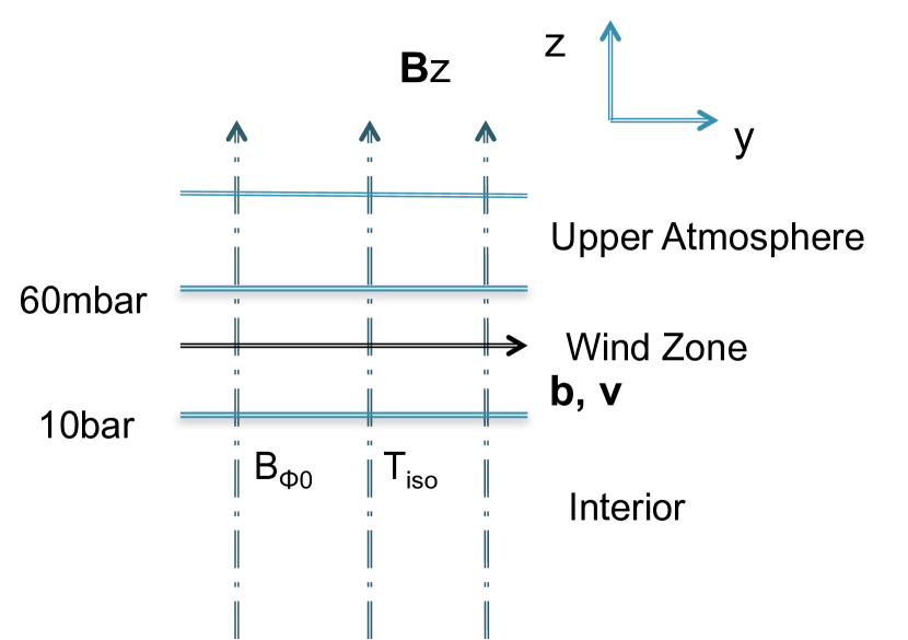
Figure 1.— The general mechanism of ohmic heating illustrated in a plane-parallel model. A vertical field $B_{z}$ is sheared by the wind $v_{y}$ in the wind zone. An induced field $b$ is produced by the shear that penetrates into the interior. We use the temperature $T_{\rm iso}$ and induced magnetic field $B_{\phi 0}$ at the base of the wind zone as boundary conditions for our interior solutions.

Some intuition about the solution can be obtained by considering a plane parallel model, which we illustrate in Figure 1. There we divide the planet into three layers, representing the outermost isothermal layer, with pressures lower than $60\ {\rm mbars}$, the wind zone, between $60\ {\rm mbars}$ and $10\ {\rm bars}$ and the interior of the planet. The vertical field $B_{z}$ is sheared by the wind with velocity $v_{y}(z)\exp{(ikx)}$. Focusing on the innermost layer representing the planet interior, and assuming constant conductivity, equation (3) gives an induced field $\vec{b}\propto\exp(-{kz}+ikx)\hat{y}$ and associated vertical current $4\pi j_{z}/c=ikb$. Both the field and current decrease exponentially in the interior on a length scale $2\pi/k$. When the variation of conductivity with depth is included, we must solve

$$\frac{d^{2}b}{dz^{2}}-k^{2}b+\frac{d\eta}{dz}\frac{db}{dz}=0,$$ (4)

in which case the thickness of the penetration depth depends on the length scale on which the conductivity varies.

This simple model illustrates that the interior solution depends on three factors: the geometry of the shearing velocity in the wind zone (which is described by $k$ in this simple model), the magnitude of the induced field at the base of the wind zone, and the profile of the electrical conductivity in the interior. The approach that we pursue in this paper is to consider the first two factors as boundary conditions on the interior. We choose to parametrize our models by specifying the toroidal magnetic field at a pressure of 10 bars, which we will refer to as $B_{\phi 0}$.

To calculate the distribution of currents inside the planet in detail, we consider a simple geometry with a dipole field and a zonal flow $\vec{v}=v_{0}\sin{\theta}\,\hat{\phi}$. To solve equation (3) in spherical coordinates we write the induced toroidal field:

$$\vec{B_{\phi}}=\frac{g(r)}{r}\sin{\theta}\cos{\theta}\hat{\phi},$$ (5)

in which case the radial dependence part of the field is given by

$$g^{\prime\prime}(r)-\frac{d\ln\sigma}{dr}g^{\prime}(r)-l(l+1)\frac{g(r)}{r^{2}}=0$$ (6)

where $l=2$ is the index of associated Legendre polynomial $P_{l}^{1}$. Having found $g(r)$ and therefore $B_{\phi}(r)$, the currents are determined by Ampère’s law $\vec{J}=(c/4\pi)\nabla\times\vec{B}$. The ohmic power in the interior is

$$P=\int\frac{J^{2}}{\sigma}\,dV\sim 4\pi\int\frac{\langle{J}\rangle^{2}}{\sigma}r^{2}\,dr,$$ (7)

where $\langle{J}\rangle=\langle{J_{r}^{2}}+J_{\theta}^{2}\rangle^{1/2}$ is the effective angle averaged current at radius $r$. To get some feeling for the dependence of the field and current on depth, we can consider a power-law dependence $\sigma\propto r^{\alpha}$. In that case, the solution is $B_{\phi}\propto r^{\beta}$ with

$$\beta=\frac{(\alpha-1)+\sqrt{(1+\alpha)^{2}+24}}{2},$$ (8)

and $\langle{J}\rangle\propto r^{\beta-1}$. For more complex wind geometries, which involve $l>2$, the solution is $\vec{B_{\phi}}\propto r^{l}P_{l}^{1}(cos\theta)$ for constant conductivity. For example, this indicates that more zonal jets in the wind zone implies a shallower penetration depth for the induced field.

In fact, as we argue in the next section (§2.2), the internal heating is dominated by the lowest densities, since the local heating rate is inversely proportional to the electrical conductivity which increases rapidly with increasing pressure. This means that the current $J$ can be taken as a constant without making a significant error in the heating profile. We have confirmed this by comparing constant current solutions with detailed solutions of equation (6).

For the constant current case, we compute the current as

$$J={c\over 4\pi}{B_{\phi 0}\over R_{J}},$$ (9)

where $R_{J}=7\times 10^{9}\ {\rm cm}$ is the radius of Jupiter, $B_{\phi 0}=B_{\phi}(r,p=10{\rm bars})$. This means that there is a direct mapping between the chosen value of $B_{\phi 0}$, the radial current inside the planet $J_{r}$, and the local heating rate, taken to be $J_{r}^{2}/\sigma(r)$ per unit volume. Note that we do not take into account the averages over angle in equation (7) nor the true radius of the planet, and so our value of $B_{\phi 0}$ for a given amount of internal heating could be a factor of a few of the toroidal field in a model which self-consistently includes both the wind zone and the interior. Instead, our parameter $B_{\phi 0}$ should be interpreted as a measure of the internal heating (given by eqs. [9] and then $J_{r}^{2}/\sigma$ locally).

2.2. Magnitude of the induced field and ohmic power

It is useful to estimate the expected magnitude of ohmic heating and how it scales with parameters such as planet mass $M$. The first step is to use equation (2) to estimate the expected strength of the induced field by dimensional analysis,

$$\frac{b}{B_{\rm dip}}=R_{M}=\frac{4\pi\sigma{H}v}{c^{2}},$$ (10)

or

$$b=B_{\rm dip}\left(\frac{\sigma}{10^{7}\,{\rm s}^{-1}}\right)\left(\frac{H}{0.01\,R_{J}}\right)\left(\frac{v}{1\,{\rm km}\,{\rm s}^{-1}}\right),$$ (11)

where $v$ is an average wind speed and $\sigma$ a typical value of electrical conductivity in the layer, and we take the vertical length scale to be the pressure scale height $H$.

In this paper, we take $B_{\rm dip}=10{\rm G}$ as a standard value. Typical dipole field strengths for hot jupiters have been estimated from scalings with planet parameters (see Trammell et al. 2011 for a detailed summary and discussion). Sánchez-Lavega (2004) argued that the field is generated by the dynamo action in the metallic region as in Jupiter (Stevenson, 1983), with the field strength closely related to the rotation of the planet, $B\sim(\rho\Omega\eta)^{\frac{1}{2}}$. This predicts that the field on typical hot jupiters should be a factor of few smaller than that on the Jupiter, with a typical value of equatorial magnetic field $B_{\rm eq}\sim 5{\rm G}$. However, Christensen et al. (2009) argue that the field instead scales with the heat flux escaping from the conductive core at large enough rotation rate, giving $B\sim(\rho{F}_{\rm core}^{2})^{\frac{1}{3}}$. This gives a field strength an order of magnitude larger than estimated with the previous method.

Given an induced field $b$, we can then estimate the expected ohmic power per unit mass, $P_{m}=\langle{J}\rangle^{2}/(\rho\sigma)$. Approximating the angle averaged current at the base of the wind zone using the constant current case as equation (9) gives

$$P_{m}=10^{-1}\ \mathrm{erg\ g^{-1}\ s^{-1}}\left(\frac{B_{\phi 0}}{10\mathrm{G}}\right)^{2}\left(\frac{\sigma}{10^{6}\ \mathrm{s}^{-1}}\right)^{-1}\left(\frac{\rho}{10^{-4}\ \mathrm{g\ cm^{-3}}}\right)^{-1}.$$ (12)

Since $\sigma$ increases dramatically in the core of the planet, heating at low density dominates. If the conductivity profile scales as $\exp(-r/H)$ for example, where we take the lengthscale as the pressure scale height $H$, the total power in the interior is

$$P_{\rm ohm,total} \approx 4{\pi}P_{\rm top}{R}^{2}\rho{H}$$ (14)

$$= 10^{23}\,\mathrm{erg\ s^{-1}}\,\left(\frac{B_{\phi 0}}{10\ \mathrm{G}}\right)^{2}\,\left(\frac{\sigma_{t}}{10^{6}\ \mathrm{s}^{-1}}\right)^{-1}\times$$

$$\left(\frac{H}{0.01\ R_{J}}\right)\left(\frac{R}{R_{J}}\right)^{2}$$

$$= 3\times 10^{22}\ \mathrm{erg\ s^{-1}}\,\left(\frac{B_{\phi 0}}{10\ \mathrm{G}}\right)^{2}\,\left(\frac{\sigma_{t}}{10^{6}\ \mathrm{s}^{-1}}\right)^{-1}\times$$

$$\left(\frac{T}{1500\ {\rm K}}\right)\,\left(\frac{R}{R_{J}}\right)^{4}\,\left(\frac{M}{M_{J}}\right)^{-1}$$

where the subscript $t$ indicates a quantity evaluated in the outermost regions of the interior just below the wind zone. Note that $H=\mathcal{R}T/g$, where we adopt $\mathcal{R}=3.64\times 10^{7}\ \mathrm{erg\ g^{-1}\ K^{-1}}$ for a hydrogen molecule dominated composition with helium fraction $Y=0.25$. As we mentioned previously, because the total ohmic power is dominated by the heating at low pressure, it is not very sensitive to the radial profile of the current. The scaling in equation (14) implies that $P_{\rm ohm}\propto 1/M$ when the radius and conductivity of planet is not strongly depend on mass, a scaling that we find in our numerical solutions. More massive planets have less ohmic power for a given $B_{\phi 0}$ and temperature $T_{\rm iso}$ at the base of the wind zone.

3. Ohmic Heating as a Function of Internal Entropy

In this section, we calculate the structure, luminosity, and ohmic heating profile for gas giants as a function of their internal entropy $S$. We will use these models in §4 to follow the time evolution of the planet by following the decreasing entropy as the planet cools. In this approach, described by Hubbard (1977) (see also Fortney & Hubbard 2003 and Arras & Bildsten 2006), it is assumed that the convective turnover time is much shorter than the evolution time of the planet, so that the convection zone maintains an adiabatic profile as it cools and lowers its entropy. We also assume that the radiative envelope has a thermal timescale much shorter than the evolution time, so that the envelope is in thermal steady-state, carrying the luminosity emerging from the convection zone. The luminosity of the planet is then given by the radiative luminosity at the radiative–convective boundary,

$$L={16\pi GcM_{r}aT^{4}\over 3\kappa p_{c}}\nabla_{\rm ad}$$ (15)

where $p_{c}$ is the pressure at the convective boundary, $T$ is the temperature at that location, and $M_{r}$ is the enclosed mass. The evolution of the internal entropy is then given by

$$\int\,T{dS\over dt}\,dm=M\bar{T}{dS\over dt}=-L(S)$$ (16)

where we have assumed $dS/dt$ is constant across the convection zone and define the mass-averaged temperature $\bar{T}=\int\,T/M\,dm$.

The effect of ohmic heating appears in two places in this approach. The first is that an ohmic heating term must be added to the right hand side of equation (16),

$$M\bar{T}{dS\over dt}=-L_{c}+\int{J^{2}\over\sigma}\,dV,$$ (17)

where the integral is over the convection zone. For a planet with a given entropy $S$, the luminosity at the top of the convection zone is fixed by the structure and is given by equation (15). However, because some of this luminosity is now provided by ohmic heating, the cooling rate of the convection zone ($dS/dt$) is smaller. The second influence of ohmic heating is that it can change the temperature profile in the radiative zone, in particular by pushing the radiative–convective boundary to higher pressure and lowering the luminosity (eq. [15]).

In this section, we include the first effect by calculating gas giant models without feedback from ohmic heating in the atmosphere (§3.1), and then include the feedback from ohmic heating in the radiative zone to include the second effect (§3.2). In §3.3, we summarize the results.

Table 1Model Summary

Model	$R(R_{J})$	$B_{\phi 0}({\rm G})$	$p_{\rm conv}({\rm bars})$	$P_{\rm ohm}({\rm erg\ s^{-1}})(p>p_{\rm conv})$	$P_{\rm ohm}({\rm erg\ s^{-1}})(p>10\ {\rm bars})$	$L_{\rm conv}(\mathrm{erg\ s^{-1}})$
Isothermal	1.25	10	62.8	$8.0\times 10^{23}$	$1.2\times 10^{25}$	$1.3\times 10^{26}$
Isothermal	1.25	100	62.8	$8.0\times 10^{25}$	$1.2\times 10^{27}$	$1.3\times 10^{26}$
Radiative	1.25	10	131.7	$6.8\times 10^{22}$	$2.8\times 10^{24}$	$7.7\times 10^{25}$
Radiative	1.25	100	131.7	$6.8\times 10^{24}$	$2.8\times 10^{26}$	$7.7\times 10^{25}$
RadiativeFB	1.25	10	132.0	$6.7\times 10^{22}$	$2.8\times 10^{24}$	$7.7\times 10^{25}$
RadiativeFB	1.25	100	176.4	$3.1\times 10^{24}$	$1.9\times 10^{26}$	$5.6\times 10^{25}$

3.1. Planet models without feedback

We now make models of gas giants with given mass $M$ and central entropy $S$, and use them to calculate the ohmic dissipation in the planet, but without including the effect of ohmic heating on the planet structure. This allows us to calculate the ohmic heating within the convection zone and, by including this ohmic power in equation (16), the corresponding slowing of the cooling rate.

We present the detail microphysics in our planet model in the Appendix A. Here we only note the differences between our opacity and conductivity profiles and those used in other works. Our opacity profile use a different extrapolation method in the intermediate pressure range between $10^{3}-10^{5}{\rm bars}$ from Paxton et al. (2011), who take the opacity for $\log R>8$ (where $R=\rho/T_{6}^{3}$ is used in the opacity tables) to be a constant set by the value at $\log R=8$. As far as we are aware, opacity calculations for this intermediate pressure range have not been carried out. For planets undergoing a large amount of internal heating, the convection zone boundary moves into this region, and so knowing the opacity there is important for understanding the location of the convection zone boundary. As we describe later, this controls the contraction rate of the cooling planet. Our potassium conductivity profile (equation [A2]) is the same as used by Perna et al. (2010a), but is different from Batygin & Stevenson (2010), who use a electron-neutron cross-section of $\pi(7.2\times 10^{-9}\ {\rm cm})^{2}=1.6\times 10^{-16}\,{\rm cm^{2}}$ rather than $10^{-15}\,{\rm cm^{2}}$ (Draine et al., 1983) and a slightly different thermal averaging factor for the velocity. The resulting difference is that the conductivity of Batygin & Stevenson (2010) is a factor of 9 times larger than our conductivity.

The planet model is calculated by integrating outwards from the center, following the convective adiabat until it intersects a radiative zone extending inwards from the surface. When calculating the cooling curve of an irradiated gas giant, a reasonable approximation is to take the outer radiative zone of the planet to be isothermal. However, because ohmic heating is very sensitive to pressure, a small error in the determination of the convective boundary results in a much larger error in the ohmic power. To illustrate this, we have calculated models with an isothermal radiative layer and with a radiative layer that is in thermal equilibrium and carries a constant luminosity equal to the luminosity from the convection zone.

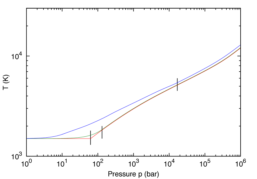
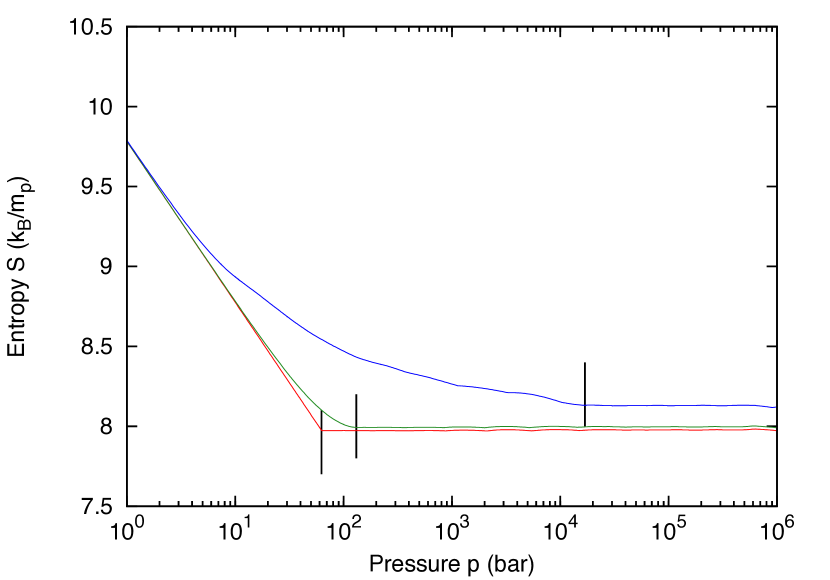
Figure 2.— The temperature profile (top panel) and entropy profile (bottom panel) for different treatments of the outer layers, either isothermal (red curve), radiative (green curve), or radiative including ohmic heating (blue curve). For the ohmic heating model, we take $B_{\phi 0}=1000\ \mathrm{G}$. In each case, the radiative–convective boundary is marked with a vertical bar. Note that we do not show the entire structure, but focus on the lower pressures to illustrate the differences in the position of the radiative–convective boundary between models.

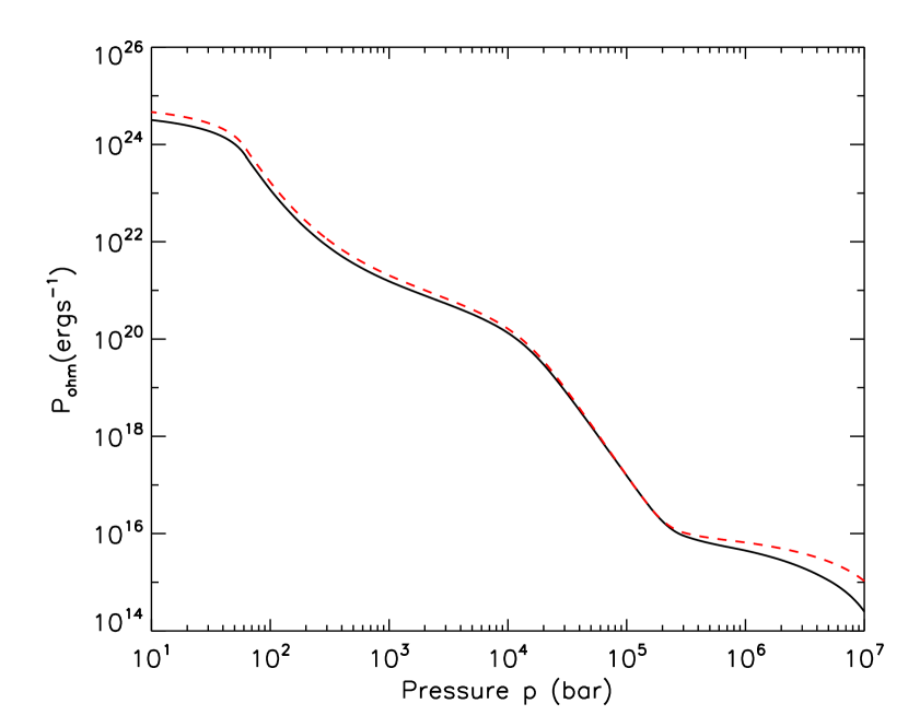
Figure 3.— The cumulative ohmic power against pressure for the same planet parameters as in Figure 17, with $B=10{\rm G}$ (radiative model, no feedback). The solid curve uses a current profile calculated by solving equation (6); the red dashed curve assumes a constant current with depth.

For the isothermal case, we integrate

$$\frac{dm}{dr} = 4\pi\rho{r^{2}}$$ (18)

$$\frac{dp}{dr} = -\rho\frac{Gm}{r^{2}}$$ (19)

$$\frac{dT}{dr} = \frac{T}{P}\nabla\frac{dp}{dr},$$ (20)

outwards from the center, taking $\nabla=\nabla_{\rm ad}$ for $T>T_{\rm iso}$ (adiabatic interior) and $\nabla=0$ for $T<T_{\rm iso}$ (isothermal layer). In the non-isothermal case, we take

$$\nabla = \min{(\nabla_{\rm rad},\nabla_{\rm ad})}$$ (21)

$$\nabla_{\rm rad} = \frac{3{\kappa}L}{16{\pi}cGM}\frac{p}{aT^{4}}.$$ (22)

We calculate a model for a given $M$ and $S$ by integrating outwards from the center and inwards from the surface to a matching pressure $p=30\ {\rm kbars}$. For the outwards integration, we choose the central pressure $p_{c}$ and cooling rate $dS/dt$ (or equivalently cooling time $t_{S}=S/\left|dS/dt\right|$). For the inwards integration, we start at a pressure of 10 bars and set the temperature there to be $T_{\rm iso}$. We then integrate inwards, choosing the luminosity $L$ and radius $R$. A multi-dimensional Newton-Raphson method is used to find the correct choices of ($p_{c},\,t_{S},\,R,\,L$) that result in $m,\,r,\,T$ and $L$ agreeing to within 1% at the matching pressure.

As an example, Figure 2 compares the entropy and temperature profiles for models with an isothermal and non-isothermal radiative zone. In the isothermal case, we choose $T_{c}=3\times 10^{4}\ {\rm K}$, $p_{c}=2\times\,10^{7}\ {\rm bars}$ and $T_{\rm iso}=1500\ {\rm K}$, which gives a $M=0.96\ M_{J}$, $R=1.25\ R_{J}$ planet with core entropy $S=7.98$ and convective zone boundary $p_{\rm conv}=62.76\ {\rm bars}$. The luminosity from the interior is $L=1.28\times\,10^{26}\ {\rm erg\ s^{-1}}$, giving $t_{S}=5.78\ {\rm Gyr}$. With a radiative zone, we obtain the same mass, radius and entropy with a convective zone boundary $p_{\rm conv}=131.7\ {\rm bars}$. The luminosity from the interior is $L=7.7\times 10^{25}\ \mathrm{erg\ s^{-1}}$, and $t_{S}=10.5\ {\rm Gyr}$ to cool.

In each case, the magnetic field structure in the planet interior is obtained by solving equation (6) using the conductivity profile in the planet (shown in Figure 17), and then the ohmic heating profile is determined. For an induced magnetic field $B_{\phi 0}=10\,{\rm G}$ at the bottom of the wind zone ($p=10\ {\rm bars}$), we find $P_{\rm ohm}(p\geqslant{p_{\rm conv}})=8\times\,10^{23}\ \mathrm{erg\ s^{-1}}$ for the isothermal model and $P_{\rm ohm}(p\geqslant{p_{\rm conv}})=6.8\times\,10^{22}\ \mathrm{erg\ s^{-1}}$ in the non-isothermal case. While the cooling time for the planet changes by a factor of two between the two models, the ohmic power changes by more than an order of magnitude. Therefore, it is crucial to locate the convective boundary accurately when calculating the ohmic power inside the convection zone.

In Figure 3, we compare the ohmic power calculated in this way, which includes the correct radial distribution of current, with the ohmic power calculated by assuming a constant radial current, independent of depth. The agreement is excellent (within a factor of 2) except at the highest pressures in the central regions of the planet.

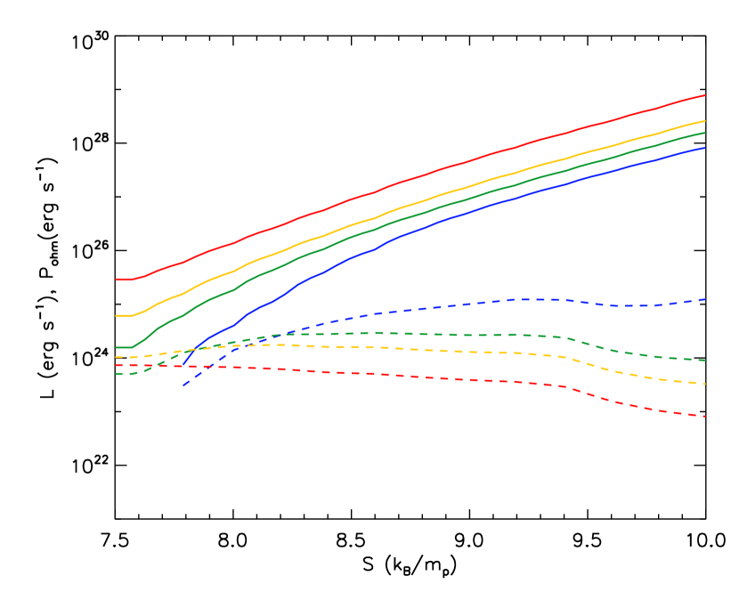
Figure 4.— The luminosity $L$ (solid curves) and the total ohmic heating in the convection zone $P_{\rm ohm}$ (dashed curves) as a function of central entropy $S$. The red, yellow, green and blue lines (from top to bottom for the solid lines; inverse for the dashed lines) represent planets with different mass: $3.0\ M_{J}$, $1.0\ M_{J}$, $0.6\ M_{J}$, $0.3\ M_{J}$. At larger entropy, where ohmic heating is unimportant, $L\propto M$ at fixed $S$, whereas $P_{\rm ohm}$ decreases with increasing $M$. All the planet models are computed with $T_{\rm iso}=1750\ {\rm K}$ and $B_{\phi 0}=100\ {\rm G}$.

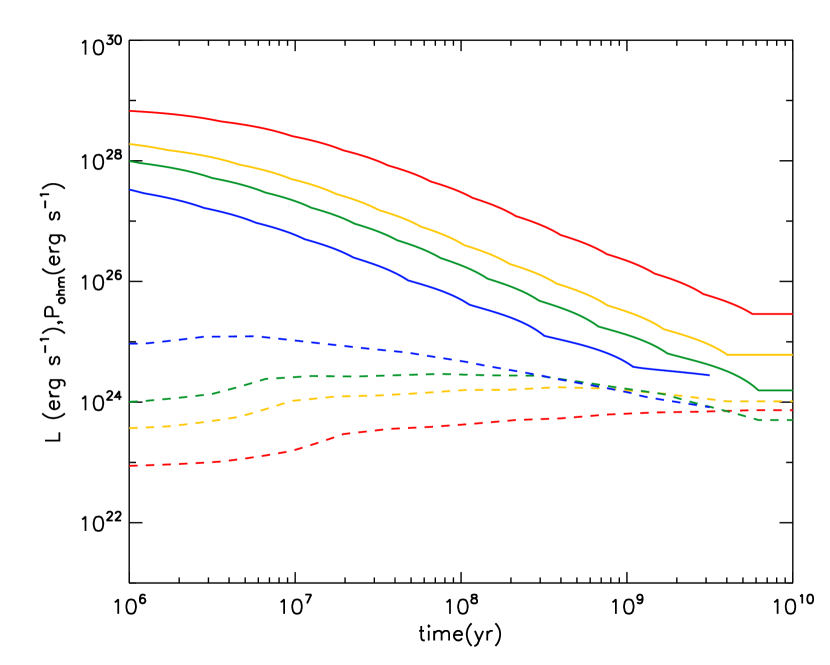
Figure 5.— The time history of planet luminosity (solid curves) and ohmic heating in the convection zone $P_{\rm ohm}$ (dashed curves) for $M=0.3\ M_{J}$ (blue), $0.6\ M_{J}$ (green), $1\ M_{J}$ (yellow) and $3\ M_{J}$ (red curves) (same configuration with Figure 4). The luminosity decreases with time because of cooling, while the ohmic heating either increases or decreases slowly depending on $M$. At late times, when ohmic heating in the radiative layer becomes important, $P_{\rm ohm}$ decreases because the convective boundary moves inwards. When $P_{\rm ohm}$ becomes comparable to $L$, the cooling and contraction of the planet is halted. All the models are calculated with $T_{\rm iso}=1750\ K$ and $B_{\phi\ 0}=100\ {\rm G}$.

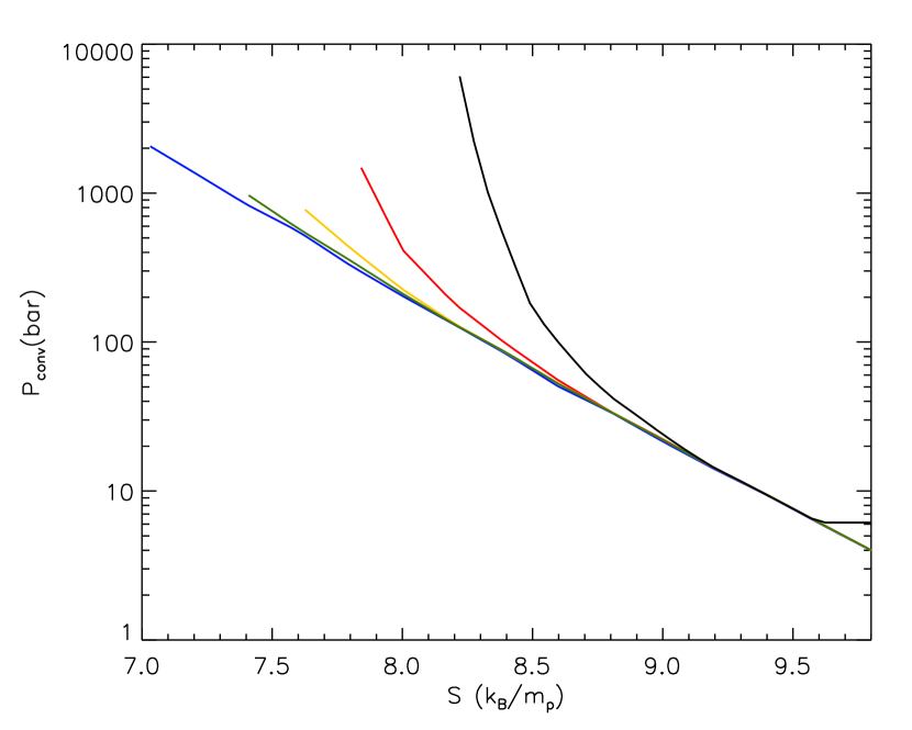
Figure 6.— Position of the radiative–convective boundary as a function of internal entropy $S$ for a $1\ M_{J}$ planet with $T_{\rm iso}=1750\ {\rm K}$. Blue, green, yellow, red, black lines are for $B_{\phi 0}=$0, 10, 30, 100, 300, 1000 ${\rm G}$. At a given entropy, a larger $B_{\phi 0}$ results in more ohmic heating in the radiative zone, moving the convective boundary to a higher pressure.

3.2. Planet models with feedback from ohmic heating

The fact that the ohmic heating per unit mass rises rapidly to lower densities (Fig. 3) suggests that the heating in the regions lying between the wind zone and the convection zone boundary will be larger than the heating in the convective interior. We include the ohmic heating in the radiative layer by allowing $L$ to vary throughout the radiative zone, with

$${dL\over dr}={J^{2}\over\sigma}.$$ (23)

We do not include ohmic heating at pressures less than 10 bars. Instead, we specify the temperature $T_{\rm iso}$ at $p=10$ bars and integrate inwards. Of course, there could be significant ohmic heating within the wind zone at $p<10$ bars, but we absorb this into the boundary condition. Note that this means that early in the lifetime of the planet, when the entropy is large enough that $p_{\rm conv}<10$ bars, the models here revert back to our previous models with no feedback. However, at those early times, ohmic heating is generally not yet important. Also note that in the models without feedback, the strength of the induced field $B_{\phi}$ does not influence the internal structure of the planet, whereas here a larger $B_{\phi}$ results in more heating in the radiative layer which can push the convective boundary deeper.

In Table 1, we compare the models with feedback to our earlier models without feedback. The internal structures are shown in Figure 2. The planet radius does not vary much between different models. The biggest difference is in the position of convective zone boundaries (marked by black vertical bars in Fig. 2), which results in a difference in the cooling luminosity and the ohmic heating both in the convective zone and atmosphere. Note that this means that the cooling history of a planet using these three approaches would be different, especially the time at which ohmic heating begins to become important for evolution. We use this feedback model for all the calculation carried on below.

3.3. Ohmic power as a function of entropy

The luminosity and ohmic power is shown as a function of entropy in Figure 4. As noted in particular by Arras & Bildsten (2006), equation (15) shows that $L\propto M$ at fixed entropy, and we see that scaling in Figure 4. On the other hand, the ohmic power decreases with increasing $M$, as discussed in §2.2. We find that the decrease in $P_{\rm ohm}$ is well described by $P_{\rm ohm}\propto R^{2.4}/M$, which has a shallower dependence on $R$ than in equation (14) because of the dependence of the conductivity term on mass which compensates the $R^{4}$ term. In our feedback model, for a lower mass planet the higher atmospheric ohmic heating pushes the convective zone boundary slightly deeper, resulting in a higher conductivity at the top of the convection zone. Overall, lower mass planets generally have higher ohmic power deposited in the convection zone.

Combined with the mass-luminosity dependence, the decrease of ohmic power with mass means that ohmic heating becomes important for lower mass planets at a much higher entropy than for more massive planets. The value of entropy at which ohmic heating becomes important depends on the boundary induced field $B_{\phi 0}$. Turning this around, for an observed planet with measured radius and mass, we can infer the entropy and therefore derive a limit on the wind zone $B_{\phi 0}$ required for ohmic heating to be providing a significant part of the luminosity in that object. We carry out this procedure in §5, but first describe our calculations of the time-evolution of planets with ohmic heating.

4. Time Dependent Evolution of Planet Structure

Having computed the luminosity at the radiative–convective boundary for a large grid of models with different $M$, $S$, $T_{\rm iso}$ and $B_{\phi 0}$, the evolution in time of a planet with fixed mass $M$, $B_{\phi 0}$ and $T_{\rm iso}$ then involves stepping in entropy using equation (17). When calculating the ohmic power, we assume constant current $J$ with depth, which as shown earlier is a good approximation. We have checked that for $B_{\phi 0}=0$, our cooling models compare well with the earlier results of Burrows et al. (1997) and Baraffe et al. (2003) (see Marleau et al. 2012). We reproduce their cooling curves to within 30% in luminosity, and predict radii that are $0.05$-$0.08\ R_{J}$ larger than in those cooling sequences.

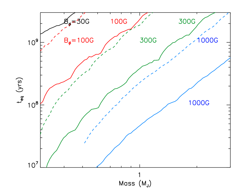
Figure 7.— The age of the planet when ohmic heating becomes important ($P_{\rm ohm}>0.1L$) versus planet mass, for $B_{\phi 0}=30\ {\rm G}$ (black), $100\ {\rm G}$ (red), $300\ {\rm G}$ (green), $1000\ {\rm G}$ (blue curves), and for two temperatures $T_{\rm iso}=1750\ {\rm K}$ (solid curves) and $2250\ {\rm K}$ (dashed curves, corresponding to the lower panel of labels).

Figure 8.— The value of $B_{\phi 0}$ required for ohmic heating to become important at an age of $3\ {\rm Gyr}$. From bottom to top, $M=$0.3, 1, 3.0 $M_{J}$.

Figure 9.— Time history of planet radius for (top to bottom) $M=$0.3, 0.6, 1 and $3\ M_{J}$. All the models are calculated with $T_{\rm iso}=1750\ {\rm K}$ and $B_{\phi 0}=100\ {\rm G}$.

By integrating in time, we compute the time history of the planet luminosity and ohmic power, shown in Figure 5. As the planet cools, the convection zone ohmic power increases or decreases slightly depending on mass, but always changes more slowly than $L$, so that ohmic power eventually becomes comparable to the cooling luminosity. At the same time, as the ohmic heating in the upper atmosphere (which is about an order of magnitude larger than convection zone heating) starts to affect the planet structure, the convective zone boundary shrinks inwards. The resulting decrease of both cooling luminosity and convection zone ohmic heating result in a rapid increase in cooling time, so that we can view the evolution afterwards as a quasi-steady state. For higher atmospheric ohmic heating, this effect happens at higher entropy, thus the steady radius of planet will be larger. We compare the evolutionary tracks of the radiative/convection zone boundary of a 1 $M_{J}$ planet with different strengths of induced field in Figure 6. As we increase the amount of ohmic heating, the convection zone boundary deviates from the no heating path at a higher entropy.

In Figure 7, we show the age of a planet with a particular mass when $P_{{\rm ohm},c}=0.1L_{\rm conv}$, at which point ohmic heating starts to become significant and the planet contraction slows. In general, the atmospheric heating is an order of magnitude larger, and so comparable to the cooling luminosity at this age. In Figure 7, we report that the result is sensitive to the strength of $B_{\phi 0}$. With $T_{\rm iso}=1750\ {\rm K}$, for $B_{\phi 0}$ equals $30\ {\rm G}$, a $0.3\ M_{J}$ hot jupiter can reach steady state in $~{}1\ {\rm Gyr}$, while a $1\ M_{J}$ requires $100\ {\rm G}$ to reach steady state at a similar age. Higher $T_{\rm iso}$ (dashed line in Figure 7) does not help the planet reach a steady-state radius faster, but on the contrary, it requires a larger induced field to achieve the same result.

Figure 8 shows the $B_{\phi 0}$ required to halt contraction within 3 Gyr as a function of $T_{\rm iso}$. We see that a hotter planet requires a stronger induced field to obtain a significant level of ohmic heating. This is because the interior ohmic heating is closely related to the conductivity at the bottom of the wind zone; the conductivity increases with temperature, reducing the ohmic heating at fixed induced field. But we should also point out that for a hotter planet there is a higher chance to obtain a stronger induced field due to the stronger wind in the atmosphere. So this result does not necessarily imply that it is more difficult to make ohmic heating important in hotter planets.

We plot the time evolution of the planet radius for planets with $B_{\phi 0}=100\ {\rm G}$ and $T_{\rm iso}=1750\,{\rm K}$ and different planet masses in Figure 9. In the absence of stellar ages, we shall take a typical age of 3 Gyr, and take the radius at $3\ {\rm Gyr}$ as the present day radius. For the lowest mass planet, $0.3M_{J}$, the effect on the evolution of the planet radius is significant, and the planet stops cooling around $1\ {\rm Gyr}$ (with cooling time longer than $10\ {\rm Gyr}$) and thereafter maintains a large radius. However, the heating is not as effective at higher masses. For example, HD 209458b has a observed radius of $1.35\ R_{J}$ with mass $0.7\ M_{J}$, while we can only obtain a radius of $1.25\ R_{J}$ for $B_{\phi 0}=100$ G. This is because the power we introduced into the planet interior is far smaller than the received stellar luminosity. In the case of our standard model, the irradiation luminosity from the host star is $10^{29}\ {\rm erg\ s^{-1}}$, and the heating in the interior is only one $0.01\%$ of it, $10^{26}\ {\rm erg\ s^{-1}}$. To go further, we must understand what values of $B_{\phi 0}$ might be expected as a function of $T_{\rm eq}$, and we turn to this in the next section.

5. Evolution including wind zone model and comparison to observations

In §4, we calculated the time-evolution of cooling gas giants assuming that $T_{\rm iso}$ and $B_{\phi 0}$ are independent parameters. In reality, they are coupled by the dynamics in the wind zone, since the atmospheric flow, in response to the irradiation, determines both the magnetic field in the layer and the temperature at depth (the values of $T_{\rm iso}$ and $B_{\phi 0}$ are specified at $p=10\ {\rm bars}$). In this section, we implement the scalings for the wind zone dynamics proposed by Menou (2012) (§5.1) and then compare our results to observed systems (§5.2).

5.1. Dynamics of the wind zone and the relation between $T_{\rm iso}$ and $B_{\phi 0}$

Both Batygin et al. (2011) and Menou (2012) write down simplified models for the wind zone dynamics including the effects of magnetic drag. In both cases, following Perna et al. (2010a) the magnetic drag force is assumed to be $\vec{J}\times\vec{B}/c$ per unit volume, with the current $\vec{J}$ set by a balance between the shearing of the magnetic field by the fluid and ohmic diffusion of magnetic field lines against the fluid motion, $\vec{J}=\sigma\vec{v}\times\vec{B}/c$ (§2). However, the dynamical balance in the two models is quite different. Menou (2012) writes the force balance for the equatorial flow as (see also Showman et al. 2010)

$$0=-\frac{v_{\phi}^{2}}{R_{P}}+\frac{\mathcal{R}{\Delta}T_{\rm horiz}\Delta\ln{p}}{R_{P}}-\frac{v_{\phi}B_{r}^{2}}{4\pi\rho\eta}.$$ (24)

The first two terms represent a balance between the advective term and the horizontal driving from the day-night temperature difference $\Delta T_{\rm horiz}$. This balance is thermal wind-like in that the horizontal pressure gradients require a vertical gradient in the fluid velocity $v_{\phi}$ over a vertical pressure scale $\Delta\ln p$. The final term represents the magnetic drag force, again integrated over a vertical scale $\Delta\ln p$. Batygin et al. (2011) on the other hand consider the meridional circulation induced by magnetic drag on the azimuthal flow, so that for example the latitudinal force balance is $fv_{y}=v_{\phi}/\tau_{L}$ where $f=2\Omega\sin\theta$ is the Coriolis parameter and $\tau_{L}$ the magnetic drag timescale. Their solution represents a thermal wind balance involving the equator-pole temperature gradient, modified by magnetic drag.

In both cases, magnetic drag limits the fluid velocity at high temperatures, where the large degree of ionization and therefore large electrical conductivity results in strong coupling of the fluid and magnetic field. Balancing the second and third terms in equation (24) gives $v_{\phi}\propto\eta$ when magnetic drag dominates, and therefore the magnetic Reynolds number $R_{M}=v_{\phi}H/\eta$ becomes almost constant, varying only slowly with temperature. Similarly, equation (16) of Batygin et al. (2011) has two possible limits, either $v_{\phi}\propto\eta$ when the lateral temperature gradient is large, in which case $R_{M}$ becomes almost constant at large $T_{\rm iso}$, or $v_{\phi}\propto\eta^{2}$ when the drag time scale is comparable to the rotation period, while the lateral gradient of temperature is still small, in which case $R_{M}\propto\eta$ declines rapidly at large $T_{\rm iso}$.

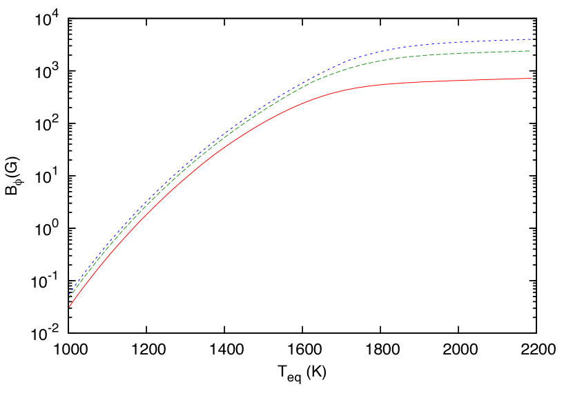
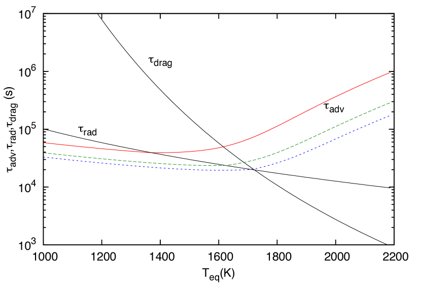
Figure 10.— The induced field $B_{\phi}$ (left panel) and timescales (right panel) in the wind zone as a function of $T_{\rm eq}$. In the left panel, the solid, dashed and dotted curves are for wind zone thickness $\Delta\ln p=0.9,3$ and $5$, and we take $B_{r}=10\ {\rm G}$. In the right panel, we show the advection, radiative and drag timescales $\tau_{\rm adv}$, $\tau_{\rm rad}$ and $\tau_{\rm drag}$. The advective timescale is shown for $\Delta\ln p=0.9$ (solid), $3$ (dashed) and $5$ (dotted curves) (the radiative and drag timescales are independent of $\Delta\ln p$).

A dynamical model including both day-night driving and meridional circulation with magnetic drag is not yet available. For our purposes, we have implemented the model of Menou (2012) as described by equation (24), with the day-night temperature difference given by

$${\Delta}T_{\rm horiz}=\cases{\frac{T_{\rm day}}{2}(\frac{\tau_{\rm adv}}{\tau_{\rm rad}})&$\tau_{\rm adv}<\tau_{\rm rad}$\cr\frac{T_{\rm day}}{2}&$\tau_{\rm adv}>\tau_{\rm rad}$\cr}$$ (25)

In equation (25), $T_{\rm day}$ is the dayside averaged temperature considering a dilution factor of 0.5, $T_{\rm irr}^{4}=2T_{\rm day}^{4}=4T_{\rm eq}^{4}$, and the advective and radiative timescales are

$$\tau_{\rm adv}=\frac{R_{P}}{v_{\phi}}$$ (26)

$$\tau_{\rm rad}=\frac{C_{p}p}{g{\sigma_{SB}}T_{\rm day}^{3}}.$$ (27)

Note that these timescales are evaluated at the outermost pressure, which following Menou (2012) is taken to be $60\ {\rm mbars}$, the estimated location of the thermal photosphere. This is the reason for adopting the thermal timescale appropriate for an optically thin region, so that $\tau_{\rm rad}\propto p$ in equation (27); in deeper, optically thick layers, $\tau_{\rm rad}$ has an extra factor of the optical depth $\tau$, leading to $\tau_{\rm rad}\propto p^{2}$ (e.g. Fig. 3 of Showman et al. 2008). The magnetic drag term is also evaluated at $p=60$ mbars; this term is integrated over height, but since $\sigma$ decreases with increasing pressure (for an isothermal layer), the dominant contribution to the integral is from the lower limit on pressure, and so $\eta$ and $\rho$ are evaluated there. This is an important difference from Batygin et al. (2011), who evaluated their magnetic drag timescale at $p=10\ {\rm bars}$, which gives a drag time an order of magnitude longer than we find here. Based on that estimate, Batygin et al. (2011) concluded that the drag timescale was always much longer than a rotation period.

We solve equation (24) for $v_{\phi}$ as a function of $T_{\rm eq}$, and find the corresponding value of the induced field $B_{\phi}$ from equation (10) for different values of the dipole field $B_{\rm dip}$. For $\Delta\ln p=0.9$, we reproduce the results of Menou (2012) (see his Fig. 1), but we also consider larger values of $\Delta\ln p$. Menou (2012) models the weather layer with a modest vertical extension around 1 pressure scale height. We also solve the equation with $\Delta\ln{p}=3$ for typical values in hot jupiter atmosphere as reported by Showman et al. (2010), and $\Delta\ln{p}=5$ for a wind zone extending to $p\sim 10$ bars, for comparison with Batygin & Stevenson (2010) and Batygin et al. (2011). The effect of varying $\Delta\ln p$ on $B_{\phi}$ is shown in the left panel of Figure 10. For numerical convenience, we fit the $B_{\phi}$–$T_{\rm eq}$ relation with the following:

$$\frac{1}{B_{\phi}(T_{\rm eq})}=\frac{1}{B_{\rm adv}}+\frac{1}{B_{\rm drag}},$$ (28)

where

$$B_{\rm adv} = 2.8\times 10^{6}\ {\rm G}\ T_{\rm eq}\exp\left(-{2.53\times 10^{4}\over T_{\rm eq}}\right)$$ (29)

$$\left({\Delta\ln{p}\over 3}\right)^{1/2}\left({B_{r}\over 10\ {\rm G}}\right)$$

and

$$B_{\rm drag}=1125\ {\rm G}\ \left({T_{\rm eq}\over 1000\ {\rm K}}\right)\left({\Delta\ln p\over 3}\right)\left({B_{r}\over 10\ {\rm G}}\right)^{-1}.$$ (30)

This reproduces $B_{\phi}$ to within $\approx 10$% for $T_{\rm eq}$ in the range $1100$ to $2200$ K.

The transition to the regime where $R_{M}$ is approximately constant occurs when $\tau_{\rm drag}$ exceeds $\tau_{\rm adv}$, where the magnetic drag timescale is $\tau_{\rm drag}=4\pi\rho\eta/B_{r}^{2}=\eta/v_{A}^{2}$, where $v_{A}$ is the Alfven speed, and again the timescale is evaluated at the top of the wind zone ($p=60$ mbars here). These timescales are plotted as a function of $T_{\rm eq}$ in Figure 10. Changing the wind zone thickness from $\Delta\ln p=0.9$ to $\Delta\ln p=5$ moves the transition temperature from $T_{\rm eq}\approx 1400$ K to 1700 K.

To use this value of $B_{\phi}$ as a boundary condition for our evolutionary models, we must relate the temperature $T_{\rm eq}$ at low pressure to the temperature $T_{\rm iso}$ at $p=10$ bars. This relation depends on the details of energy transport in the wind zone, including the effects of ohmic heating and needs to be studied further. Here, we adopt the atmospheric temperature profile from Guillot (2010), and keep in mind the uncertainty in the relation between $T_{\rm eq}$ and $T_{\rm iso}$ when interpreting our results below. The relation from Guillot (2010) is (see his eq. [29])

$$T^{4}=\frac{3T_{\rm irr}^{4}}{4}f\left[\frac{2}{3}+\frac{1}{\gamma\sqrt{3}}\right],$$ (31)

where $\gamma$ is the ratio between visible and infra-red opacities, and $f=1/2$ for a dayside average or $f=1/4$ for an average over the whole surface. Choosing $\gamma=0.4$, as appropriate for a planet like HD 409658b (e.g. see Fig. 1 of Hubeny et al. 2003) and a dayside average $f=0.5$, we obtain $T_{\rm iso}=0.94T_{\rm irr}=1.33T_{\rm eq}$. In the following section, we will use this relation to infer the appropriate value of $T_{\rm iso}$ from the $T_{\rm eq}$ of observed planets. We note here that we don’t have a good knowledge of what the $\gamma$ parameter would be for most of the observed planets. While $\gamma$ parameter could vary in a very large numerical range, the ratio between $T_{\rm iso}$ and $T_{\rm eq}$ only changes within a factor of few [$0.99(\gamma\to\inf)<(T_{\rm{iso}}/T_{\rm{eq}})<3.05(\gamma=0.01)$]. Since the observed properties of planets gives $T_{eq}$ thus the boundary induced field, changing the value $T_{\rm iso}/T_{\rm eq}$ is equivalent to shift inside the plane $T_{\rm iso}-B_{\phi}$ given by Figure 8. Generally, a smaller $T_{\rm iso}/T_{\rm eq}$ is favored to inflate the planet with the same $B_{\phi}$.

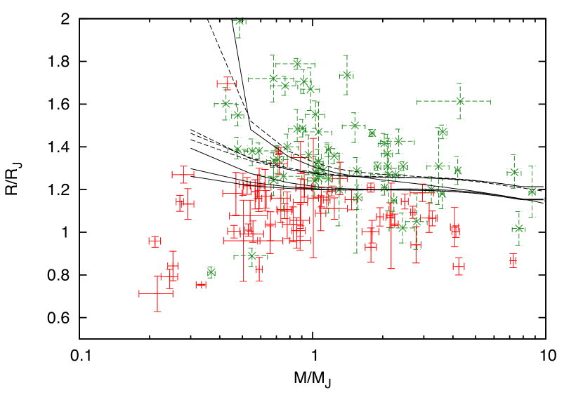
Figure 11.— The predicted mass–radius relation at $3\ {\rm Gyr}$ for $B_{\phi 0}=$0, 30, 100 and $1000\ {\rm G}$ and $T_{\rm eq}=1316\ {\rm K}$ (solid curves) and $1692\ {\rm K}$ (dashed curves). The data points show observed transiting planets, divided into two temperature groups $T>1500\ {\rm K}$ (green points) and $T<1500\ {\rm K}$ (red points).

5.2. Comparison with Observed Hot Jupiters

In Figures 11 to 13, we compare our results with the observed properties of transiting planets taken from the TEPcat transiting planet catalog, which gives the planet mass, radius, and equilibrium temperature $T_{\rm eq}=T_{\star,{\rm eff}}\,(R_{\star}/2a)^{1/2}$ where $T_{\star,{\rm eff}}$ is the stellar effective temperature. As the ages of most stars are unknown or highly uncertain, we assume an age of 3 Gyr when comparing with the observed planets.

First, Figure 11 shows the effect of increasing $B_{\phi 0}$ at fixed $T_{\rm iso}$ on the planet radius. To help compare with the data, we divide the observed sample into two groups with either $T_{\rm eq}>1500\ {\rm K}$ (green points) or $<1500\ {\rm K}$ (red points) and show theoretical curves for either $T_{\rm eq}=1316\ {\rm K}$ or $1692\ {\rm K}$ (these two temperatures correspond to $T_{\rm iso}=1750$ and $2250\ {\rm K}$ respectively). We see that for the low $T_{\rm eq}$ group, an induced field of 10–100 G can explain most of the observed radii, while the high $T_{\rm eq}$ planets need at least $B_{\phi 0}=1000\ {\rm G}$ to match the observed radii. It is clear that a higher induced magnetic field is needed to explain a given radius at higher equilibrium temperature.

Next, we use the wind zone model described in §5.1 to calculate $B_{\phi 0}$ as a function of $T_{\rm eq}$, assuming canonical values $B_{r}=10\ {\rm G}$ and $\Delta\ln{p}=3$. In the top panel of Figure 12, we show the radius as a function of $T_{\rm eq}$, with the colors representing three different bins in planet mass. There exists a clear correlation between the radius and $T_{\rm eq}$, both in the observations and the models. In addition, we see that the amount of inflation is also strongly dependent on the planet mass. Planets within the mass bin 0.3–0.6 $M_{J}$ agree quite well with our ohmic heating model. However, ohmic heating clearly cannot explain planets with mass $\sim 1\ M_{J}$ and large inflated radii $\gtrsim 1.4\ R_{J}$. Ohmic heating can help to increase the radius (for comparison the dashed line shows models with no ohmic heating), but not enough to match the observed value. This is a consequence of the increased power needed to maintain the radius of a massive planet at a particular value, as well as the reduced ohmic heating power at larger masses.

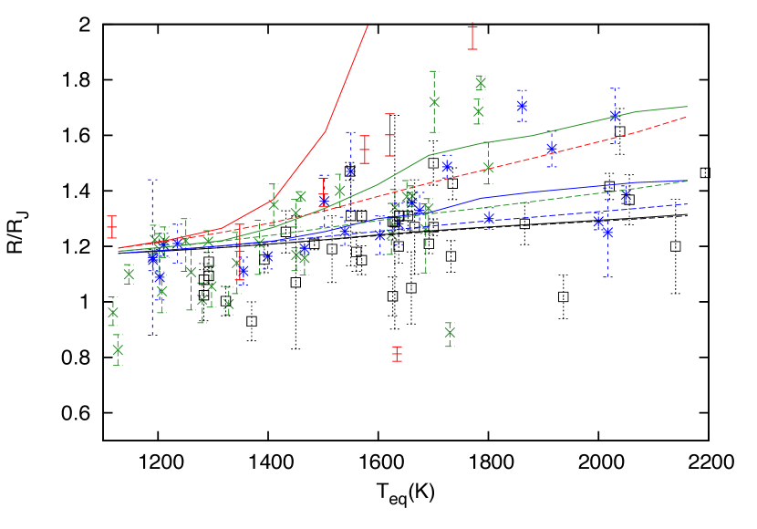
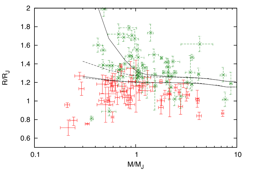
Figure 12.— Comparison with observations using $B_{\phi 0}(T_{\rm eq})$ from the wind zone model. Top panel: Radius at 3 Gyr against $T_{\rm eq}$ for $M=0.3$ (red), $0.6$ (green), $1.0$ (blue) and $3.0\ M_{J}$ (black). The data points are observed planets divided by mass: $0.2\ M_{J}<M<0.5\ M_{J}$ (red points), $0.5\ M_{J}<M<0.9\ M_{J}$ (green points), $0.9\ M_{J}<M<1.3\ M_{J}$ (blue points). Bottom panel: Predicted mass–radius relation at $3\ {\rm Gyr}$ for $T_{\rm eq}=1316\ {\rm K}$ and $T=1682\ {\rm K}$ (bottom to top). In each case, the dashed curve shows the radius without ohmic heating; the solid curve with ohmic heating. The data has been divided by temperature: $T_{\rm eq}<1500\ {\rm K}$ (red points), $T>1500\ {\rm K}$ (green points).

In the lower panel of Figure 12, we show the radius as a function of mass. As in Figure 11, we divide the data into two temperature ranges and show the model results for two representative temperatures, now using the wind zone model to specify the value of $B_{\phi 0}$ for each temperature. The parameter region where ohmic heating has the largest effect is high temperature, low mass planets. The radii of the low temperature group ($T_{\rm eq}<1500$ K) can almost all be explained without ohmic heating. For the high temperature group, ohmic heating can explain the observed radii of low mass planets, but most of the radii of the high temperature group lie well above the models, especially at large planet masses $\gtrsim 1\ M_{J}$.

In Figure 13, we show the ratio between observed and predicted radii $R_{\rm obs}/R_{\rm pred}$ against $T_{\rm eq}$ (upper panel) and against $M$ (lower panel) for each observed planet. In this case, we use the observed values of $M$ and $T_{\rm eq}$ to calculate the evolution of the planet, and, in the absence of stellar ages, we take $R_{\rm pred}$ to be the radius at 3 Gyr. In the upper panel, we see that for $T_{\rm eq}\gtrsim 1600\ {\rm K}$, there are many planets whose radii lie above the predicted values. The slow increase of $B_{\phi 0}$ with $T_{\rm iso}$ at large $T_{\rm iso}$ due to the magnetic drag term results in a much weaker dependence of $R_{\rm pred}$ on $T_{\rm eq}$ than observed, and most outliers lie at the highest temperatures. In the lower panel, we see that the majority of the unexplained objects ($R_{\rm obs}>R_{\rm pred}$) are at larger masses $M\gtrsim 0.7\ M_{J}$. We note that the choice of estimating the planet radius at $3\ {\rm Gyr}$ is not critical for the above picture. Constraining ourself within the time range of $1-5\ {\rm Gyr}$, the predicted radius only varies within several percent.

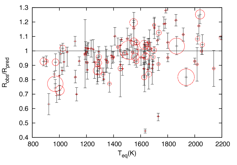
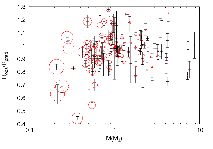
Figure 13.— The ratio of observed planet radius $R_{\rm obs}$ and predicted radius $R_{\rm pred}$ (3 Gyr) for observed hot jupiters as a function of $T_{\rm eq}$ (upper panel) or $M$ (lower panel). In the upper panel, the size of the circle scales with planet mass; in the lower panel, the size of the circle scales with $T_{\rm eq}$.

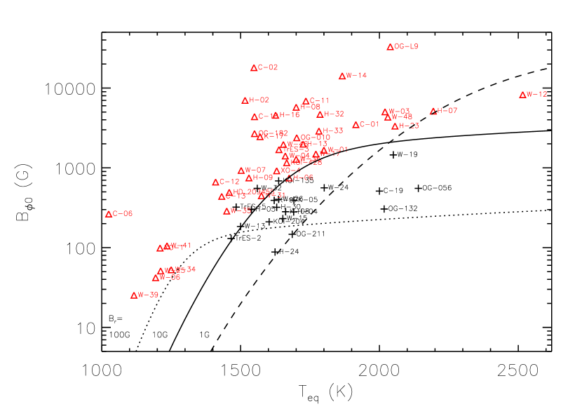
Figure 14.— For each observed planet, we show the $B_{\phi 0}$ required for ohmic heating in the convection zone to be 30% of the luminosity as estimated from no-feedback planet models, and compare with the results of our time-dependent calculations with feedback included. The curves show the $B_{\phi 0}$–$T_{\rm eq}$ predicted by the wind zone model for three different values of $B_{r}$. Black points show planets whose radii can be explained by our model ($R_{\rm pred}>R_{\rm obs}$ in Fig. 13), red points show planets that cannot be explained ($R_{\rm pred}<R_{\rm obs}$ in Fig. 13). For clarity, we use the following abbreviations for planet names: W–WASP; H–HAT-P; K–Kepler; OG–OGLE-TR; C–CoRoT-P.

To look in more detail at the effect of our assumed wind zone model on how successfully we are able to reproduce the observed radii, in Figure 14 we show the results in the $B_{\phi 0}$–$T_{\rm eq}$ parameter space. For each observed planet, we first make a model with no ohmic heating, varying the internal entropy $S$ at the measured $M$ and $T_{\rm eq}$ until we match the measured radius $R_{p}$. Then we calculate the value of $B_{\phi 0}$ required in that model for the ohmic power in the convection zone $P_{\rm ohm}$ to be 30% of the planet’s luminosity. We colour-code the data points according to whether they are successfully explained by our time evolutions, ie. whether they have $R_{\rm pred}$ larger or smaller than $R_{\rm obs}$ in Figure 13. These two groups of data points lie on either side of the $B_{\phi 0}$–$T_{\rm eq}$ relation from the wind zone model (solid curve). This shows that the approach of using a structural model with no ohmic heating (we refer to this as a “no feedback” model in §3) to estimate the critical magnetic field is a good approximation of our detailed time-evolution models including feedback.

Comparing the red points in Figure 14 with the solid curve gives a sense of how far short the ohmic heating model falls in explaining the most inflated planets. For example, HAT-P-32 is about a factor of $3$–$4$ above the curve, so that the heating rate ($\propto B^{2}$) needs to be increased by about an order of magnitude to explain the observed radius. It is interesting that most of the unexplained objects lie within a factor of 3 in terms of $B_{\phi 0}$ of the wind zone model. Figure 14 helps to show what changes to the wind zone model would explain more of the observed objects. We have assumed the relation $T_{\rm iso}=1.33T_{\rm eq}$ (from eq. [31]); a larger factor between $T_{\rm iso}$ and $T_{\rm eq}$ would move the solid curve to the left, allowing ohmic heating to explain the radii of low $T_{\rm eq}$ planets such as WASP-06. The dashed and dotted curves show the effect of changing $B_{r}$. Increasing $B_{r}$ from 10 to 100 G does increase $B_{\phi 0}$ at low temperatures, but reduces $B_{\phi 0}$ at high temperatures where magnetic drag is enhanced. A larger depth $\Delta\ln P$ would help to reduce the number of discrepant objects since both $B_{\rm adv}$ and $B_{\rm drag}$ increase with $\Delta\ln P$ (eqs. [29] and [30]).

6. Summary and Discussion

In this paper, we present models of ohmic heating in hot jupiters in which we attempt to decouple the interior and wind zone by replacing the wind zone by a boundary temperature $T_{\rm iso}$ and magnetic field $B_{\phi 0}$, both evaluated at a pressure $p=10$ bars. This approach allows us to survey the outcomes of ohmic heating, parametrized by $T_{\rm iso}$ and $B_{\phi 0}$ for planets with different mass $M$. This is similar in spirit to models of gas giant cooling, which often set an outer boundary pressure of 10 bars and separately integrate a $T_{10}$–$T_{\rm eff}$ relation to use as an outer boundary condition.

The main conclusions of the paper are:

1. Figure 4 is a key result, showing as a function of entropy how the ohmic power compares to the planet luminosity. Only planets with entropy below a critical value have enough ohmic heating to slow their contraction rate. Of particular note are the different mass dependences: at fixed $B_{\phi 0}$ and $T_{\rm iso}$, the cooling luminosity $L\propto M$ whereas the ohmic power decreases with mass (we find $P_{\rm ohm}\propto R^{2.4}/M$).

2. Ohmic heating has two effects on the thermal state of the planet. As well as providing direct heat input into the adiabatic convective interior (as found by previous works, see Batygin & Stevenson (2010); Perna et al. (2010b); Wu & Lithwick (2012)), the feedback of ohmic heating in the region between the wind zone and the convective boundary moves the convective zone boundary deeper (Fig. 6), leading to a reduced cooling luminosity and reduced internal ohmic heating. Because the electrical conductivity changes dramatically with pressure through the planet, the total ohmic power inside the convection zone is very sensitive to its radial extent. To computing the planet age and radius at the late stage when ohmic heating halted the cooling, it is crucial to accurately locate the convective-radiative boundary.

3. A larger $B_{\phi 0}$ is required for ohmic heating to be important in more massive planets or planets with larger $T_{\rm eq}$. This can be seen in Figures 7 and 8, which show the age of a cooling gas giant when ohmic heating becomes important, and the magnetic field strength required for ohmic heating to be important at different values of $T_{\rm iso}$. For example, at a temperature $T_{\rm iso}=1750\ {\rm K}$, Figure 8 shows that $B_{\phi 0}\approx 30\ {\rm G}$ will halt the contraction of a $0.3\ M_{J}$ planet in 3 Gyr, whereas $B_{\phi 0}\approx 150\ {\rm G}$ is required for a $1M_{J}$ planet at that temperature. At higher $T_{\rm iso}=2250\ {\rm K}$, the required values are $B_{\phi 0}\approx 100\ {\rm G}$ for a $0.3M_{J}$ planet or $B_{\phi 0}\approx 700\ {\rm G}$ for a $1M_{J}$ planet.

4. With a specific model for the wind zone (§5.1), we can compare to observed systems as a function of their observed equilibrium temperatures $T_{\rm eq}$. The wind zone model specifies the induced field $B_{\phi 0}$ (or equivalently, the radial current that penetrates into the interior; see eq. [9]) as a function of $T_{\rm eq}$, and the relation between $T_{\rm eq}$ and the temperature at $10\ {\rm bars}$. Using the scaling analysis proposed by Menou (2012) for the dynamics of the wind zone, together with the atmospheric temperature profile from Guillot (2010), we find that it is difficult for ohmic heating to explain the large radii of hot jupiters with large masses and large $T_{\rm eq}$ (see Fig. [13]).

5. A more general approach is to calculate, for each observed planet, the $B_{\phi 0}$ that is required if ohmic heating is providing a significant fraction of the luminosity (and therefore able to significantly change the contraction rate of the planet). This is shown in Figure 14 and shows how much the heating rate needs to be increased over the wind zone model in §5.1 to explain particular objects. A modest increase in the wind zone thickness over that assumed here, or larger ratio of the temperature at depth $T_{\rm iso}$ compared to $T_{\rm eq}$, would improve the agreement with observed radii (see discussion in §5.2). Even so, several objects require a much more dramatic increase in heating rate (see Fig. 14).

The difficulty in explaining many of the observed radii that we have found differs from Batygin et al. (2011) and Wu & Lithwick (2012) who found that they could account for almost all of the observed hot jupiter radii with ohmic heating. The key difference is that we do not assume here that the heating efficiency (the fraction of the irradiation going into ohmic power, typically taken to be $\epsilon\sim 1$%) to be fixed, but instead use the wind zone model to set the induced magnetic field in the wind zone and therefore the magnitude of the heating.

It is important to emphasize that our conclusions about the efficacy of ohmic heating depend on the particular prescription for the magnetic field in the wind zone that we have used. In fact, many complexities underlie the path from the irradiation to the properties of the induced magnetic field. More realistic 3D wind zone models may give a different picture than the simple 1D force balance scalings we have used here. For example, in this paper we have assumed the wind zone extends to p = 10 bars. Figure 3 of Wu & Lithwick (2012) nicely illustrates the importance of the depth of the wind zone, showing that a shallower wind zone requires a significantly larger overall efficiency to achieve the same interior heating. One situation in which this will break down is for young planets with high entropies when the radiative/convective zone boundary is at lower pressure. More work is needed on what happens when the interior convection zone extends into the wind zone region.

Our results emphasize the key inputs that are necessary from atmospheric models: the thermal structure and dynamics of the wind zone including a large scale magnetic field, the values of induced magnetic field, or equivalently the magnetic Reynolds number $R_{M}$, that can be attained there, and the depth of the wind zone. More studies of the local conductivity profile and magnetic field properties in the high magnetic Reynolds number regime are needed. In particular, it is not clear whether the large values of induced field $B_{\phi 0}>1000\ {\rm G}$ needed to explain the observed radii (Fig. 17) can be achieved in the wind zone. Furthermore, whether the implied large internal currents affect the planetary dynamo is also an open question.

Our results do compare favorably with previous calculations if we use equation (11) to set a value of $B_{\phi 0}$ appropriate for the wind zone conditions assumed in those papers. For example, we are able to compute the $3\%$ heating profile at pressures $p>10\ {\rm bars}$ in Figure 4 of Batygin & Stevenson (2010) by setting $B_{\phi 0}=300\ {\rm G}$; we reproduce the heating profile of Tres-4b from Wu & Lithwick (2012) with $B_{\phi 0}\approx 1500\ {\rm G}$. However, a complication in comparing different models is that the heating dissipated in the wind zone is coupled with the heating dissipated in the planet interior. Wu & Lithwick (2012) in particular discuss the expected ratio of heating deposited in different layers. But this ratio is generally model dependent and varies through the planet lifetime. A direct result of this kind of coupling is that models with same heating efficiency but different wind zone model are not physically comparable. For example, for a given set of planet properties, the radius predicted by Batygin & Stevenson (2010) is larger than in Wu & Lithwick (2012) for the same choice of heating efficiency $\epsilon$, because the heating ratio between the wind zone and the interior is much smaller in Batygin & Stevenson (2010), creating a much stronger internal heat source. Similarly, although Menou (2012) estimated the total ohmic heating efficiency to be $>1\%$ over a certain range of equilibrium temperatures (with the weather layer between $60$ mbars and $150$ mbars), the internal heating has a much lower efficiency, consistent with our findings in §5.

Another uncertainty is in the microphysics aspects of the electrical conductivity. For example, as we noted in §3.1, Batygin & Stevenson (2010) make a different choice for the electron-neutral cross-section and thermal averaging that results in a factor of 9 difference in electrical conductivity than we adopt here. The estimates in §2.2 show that the amount of ohmic power is sensitive to changes in the electrical conductivity (or the ionization fraction) in two ways. At low densities in the wind zone, the conductivity determines the size of the current (eq. [10]); in the interior, the ohmic power is $\propto 1/\sigma$ (eq. [14]). For a fixed efficiency $\epsilon$, a different normalization for $\sigma$ does not change the evolution of the planet, since the normalization of the heating profile is determined by the choice of $\epsilon$, and $\sigma(r)$ determines only its shape. The normalization of $\sigma$ is important, however, when going beyond the constant efficiency assumption, making it crucial to understand the processes that set the ionization level in hot jupiter atmospheres.

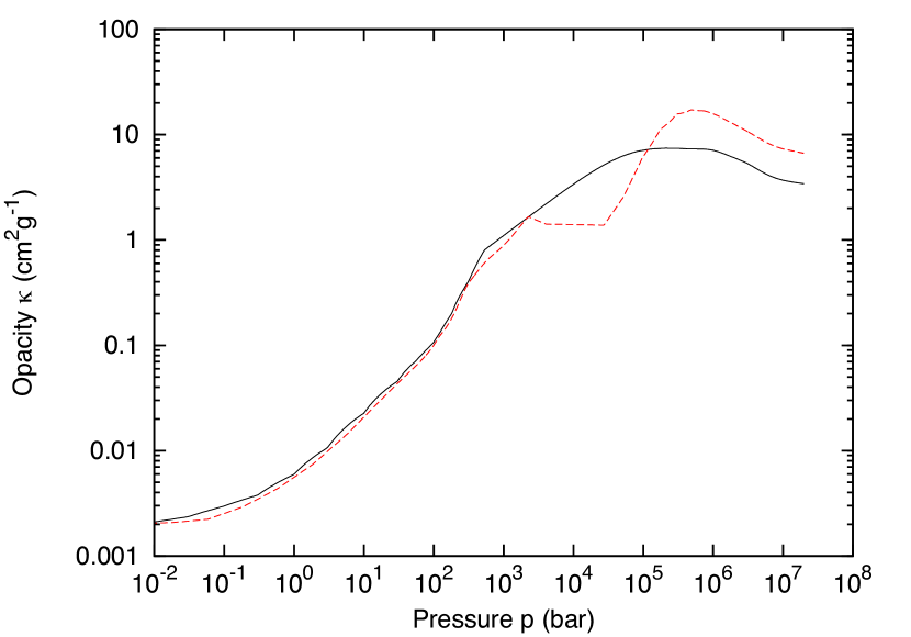
Figure 15.— The opacity profile in a planet with parameters as in Table 1 tablenote a (no ohmic heating, radiative model), showing the opacity as calculated by combining the Freedman et al. (2008) and Potekhin & Chabrier (2010) tables (solid curve) or from the MESA code (Paxton et al., 2011) (red dashed curve).

Figure 16.— The contribution to the electron fraction $Y_{e}$ from different alkali metals as a function of temperature and pressure. Solid curves are for potassium, dotted for sodium, and dashed for aluminum. In each case, we show (top to bottom) pressures of 1, 100 and 1000 bars.

Appendix A Microphysics of the planet interior

We discuss the microphysics input in our gas giant models here. We adopt the equation of state from Saumon et al. (1995) with helium fraction $Y=0.25$. In order to maximize the planet radius, we do not include a solid core or elements heavier than helium.

The radiative opacity is taken from Freedman et al. (2008) and in the core we include thermal conduction by electrons from Potekhin & Chabrier (2010). The transition from radiative to conducive opacity occurs at a pressure which is greater than the maximum pressure of 300 bars covered by the Freedman et al. (2008) tables. In the intermediate regime, we assume the scaling $\kappa\propto{p}^{0.5}$. The opacity profile for our standard model is shown in Figure 15, over-plotted with opacity taken from MESA using the same planet structure (Paxton et al., 2011).

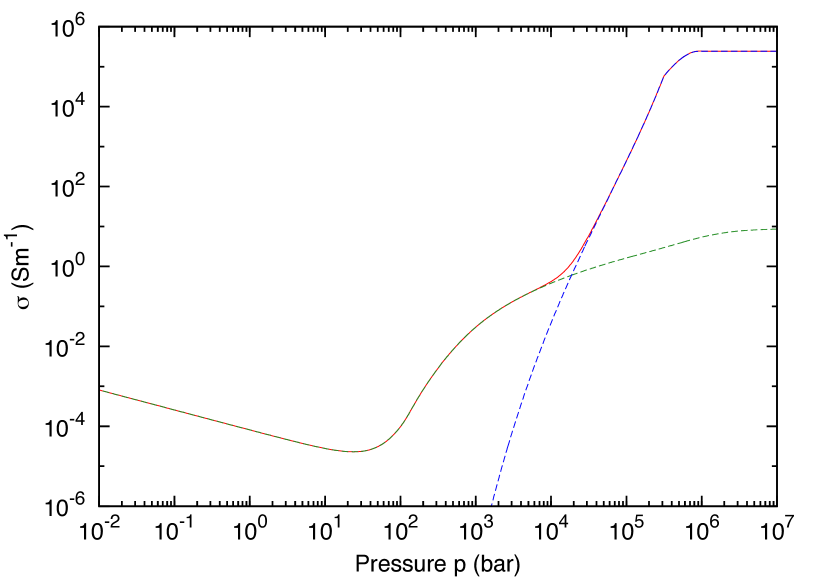
Figure 17.— Top panel: the electrical conductivity profile of a planet with parameters as in Table 1 tablenote a (no ohmic heating, radiative model), showing the contributions from alkali metals (dashed green curve) and hydrogen (dashed blue curve). Bottom panel: the electron fraction $Y_{e}$ as a function of pressure, with the contribution from alkali metal ionization shown as a dashed curve.

The electrical conductivity has contributions from alkali metal ionization in the outer layers, and hydrogen in the interior. In the upper atmosphere of hot jupiters, the conductivity is set by the ionization of alkali metals. For potassium, which has the lowest ionization potential . The potassium only Saha equation (Balbus & Hawley, 2000; Perna et al., 2010a) gives the ionization fraction $x_{k}=n_{e}/n$ as

$$x_{k}=\left[\frac{f_{k}}{n}\left(\frac{m_{e}k_{B}T}{2\pi\hbar^{2}}\right)^{3/2}e^{-4.35{\rm eV}/k_{B}T}\right]^{\frac{1}{2}}$$ (A1)

$$=1.03\times 10^{-3}\ T_{3}^{5/4}e^{-25.19/T_{3}}\left(\frac{f_{K}}{10^{-7}}\right)^{1/2}\left(\frac{p}{1{\rm bar}}\right)^{-1/2},$$

where $f_{K}$ is the number fraction of potassium. Although potassium dominates, we also include the contribution of Na, Mg, and Fe in the ionization balance to sum up the total ionization fraction. The ionization fraction of each alkali metal is computed separately by assuming a balance independent on the presents of other elements . We do not include the contribution of Al in the calculation, which is likely condensed out (Lodders, 1999). But our results are not very sensitive to elements beyond potassium. This is illustrated in Figure 16 which shows the contributions to the ionization level from K, Na and Al at different pressures. Once the ionization fraction is determined, the conductivity is $\sigma=n_{e}e^{2}/m_{e}\nu$ where the collision frequency of electron-neutral collisions is $\nu_{\rm en}=n_{n}\langle\sigma{v}\rangle_{e}$ given by Draine et al. (1983) as

$$\langle\sigma{v}\rangle_{e}=10^{-15}\left(\frac{128k_{B}T}{9\pi{m_{e}}}\right)^{1/2}\ {\rm cm}^{3}\ {\rm s}^{-1}.$$ (A2)

The conductivity is then

$$\sigma=8.8\times 10^{-2}\ {\rm S\ m^{-1}}\ \left({x\over 10^{-7}}\right)\left({T\over 1500\ {\rm K}}\right)^{-1/2}.$$ (A3)

In the deeper part of the planet, the hydrogen is ionized by high pressure and the conductivity is dominated by electron-proton collisions. In the fully-degenerate limit, $\nu_{\rm epd}=4e^{4}m_{e}\Lambda/3\pi\hbar^{2}=1.8\times\,10^{16}\,{\rm s}^{-1}$. In the non-degenerate limit, $\nu_{\rm epnd}=6.4\times 10^{23}\ s^{-1}\rho{Y_{e}}T^{-3/2}$, in which $Y_{e}$ is the electron fraction. We interpolate between the two limits to give an estimation of the total contribution: $\nu_{\rm ep}^{-2}=\nu_{\rm epd}^{-2}+\nu_{\rm epd}^{-2}$. We also include the conductivity at intermediate densities as given by Liu et al. (2006). Before the hydrogen molecule is fully ionized, the band-gap of hydrogen will diminish with increasing pressure, to a level where there is a significant contribution to the conductivity. Liu et al. (2006) give this as

$$\sigma_{s}=\sigma_{0}\exp\left(\frac{-E_{g}(\rho)}{k_{B}T}\right)$$ (A4)

where between 0.2 Mbars and 1.8 Mbars, $E_{g}=20.3-64.7\rho$, where $E_{g}$ is in eV, and $\rho$ is in ${\rm mol}\,{\rm cm}^{-3}$, and $\sigma_{0}=3.4\times 10^{20}\ \mathrm{s}^{-1}\ \exp(-44\rho)$. The overall conductivity is constructed as $\sigma=\sigma_{s}+n_{e}\,e^{2}/m_{e}\nu=\sigma_{s}+1.52\times 10^{32}\rho{Y_{e}}/\nu$. The collisional frequency $\nu$ is the sum of electron-neutral and electron-proton collisions. A typical conductivity profile and the contribution of different components are shown in Figure 17.

References

- Arras & Bildsten (2006) Arras, P., & Bildsten, L. 2006, ApJ, 650, 394
- Balbus & Hawley (2000) Balbus, S. A., & Hawley, J. F. 2000, Space Sci. Rev., 92, 39
- Baraffe et al. (2003) Baraffe, I., Chabrier, G., Barman, T. S., Allard, F., & Hauschildt, P. H. 2003, A&A, 402, 701
- Baraffe et al. (2010) Baraffe, I., Chabrier, G., & Barman, T. 2010, Reports on Progress in Physics, 73, 016901