8 (3:08) 2012 1–28 Dec. 1, 2011 Aug. 10, 2012
*A short version of this work has appeared in the Proceedings of the 26th Annual IEEE Symposium on Logic in Computer Science (LICS), 2011
Isomorphisms of types in the presence of higher-order references\rsuper*
Abstract.
We investigate the problem of type isomorphisms in the presence of higher-order references. We first introduce a finitary programming language with sum types and higher-order references, for which we build a fully abstract games model following the work of Abramsky, Honda and McCusker. Solving an open problem by Laurent, we show that two finitely branching arenas are isomorphic if and only if they are geometrically the same, up to renaming of moves (Laurent’s forest isomorphism). We deduce from this an equational theory characterizing isomorphisms of types in our language. We show however that Laurent’s conjecture does not hold on infinitely branching arenas, yielding new non-trivial type isomorphisms in a variant of our language with natural numbers.
Key words and phrases:
Isomorphisms of types, general references, game semantics1991 Mathematics Subject Classification:
F.3.21. Introduction
During the development of denotational semantics of programming languages, there was a crucial interest in defining models of computation satisfying particular type equations. For instance, a model of the untyped -calculus can be obtained by isolating a reflexive object (that is, an object such that ) in a cartesian closed category. In the 80s, some people started to consider the dual problem of finding these equations that must hold in every model of a given language: they were coined type isomorphisms by Bruce and Longo. In [8], they exploited a theorem by Dezani [9] giving a syntactic characterization of invertible terms in the untyped -calculus to prove that that the only isomorphisms of types present in simply typed -calculus with respect to equality are those induced by the equation . Later this was extended to handle such things as products [7], polymorphism [8], possibly with unit types [10], or sums [12].
The interest in type isomorphisms grew significantly when their practical impact was realized. In [26], Rittri proposed to search functions in software libraries using their type modulo isomorphism as a key. He also considered the possibilities offered by matching and unification of types modulo isomorphisms [27]. A whole line of research has also been dedicated to the study of type isomorphisms and their use for search tools in richer type systems (such as dependent types [5]), along with studies about the automatic generation of the corresponding coercions [4]. Such tools were implemented for several programming languages, let us mention the command line tool camlsearch written by Vouillon for CamlLight. The interested reader may refer to the nice survey by Di Cosmo [11].
It is worth noting that even though these tools are written for powerful programming languages featuring complex computational effects such as higher-order references or exceptions, they rely on the theory of isomorphisms in weaker (purely functional) languages, such as the second-order -calculus with pairs and unit types for camlsearch. Clearly, all type isomorphisms in -calculus are still valid in the presence of computational effects (indeed, the operational semantics are compatible with ). What is less clear is whether those effects allow the definition of new isomorphisms. However, it seems that syntactic methods deriving from Dezani’s theorem on invertible terms in -calculus cannot be extended to complex computational effects. The base setting itself is completely different: there is no longer a canonical notion of normal form, the natural equality between terms is no longer convertibility but observational equivalence, so new methods are required.
In [20], Laurent introduced the idea of applying game semantics to the study of type isomorphisms (although one should mention the precursor characterization of isomorphisms by Berry and Curien [6] in the category of concrete data structures and sequential algorithms). Exploiting his earlier work on game semantics for polarized linear logic [19], he found the theory of isomorphisms for LLP from which he deduced (by translations) the isomorphisms for the call-by-name and call-by-value -calculus. The core of his analysis is the observation that isomorphisms between arenas and in the category [14] of arenas and innocent strategies are in one-to-one correspondence with forest isomorphisms between and , so in particular two arenas are isomorphic if and only if their representations as forests are identical up to the renaming of vertices.
From the point of view of computational effects this looks promising, since game semantics are known to accommodate several computational effects such as control operators [17], ground type [2] or higher-order references [1] or even concurrency [18] in one single framework. Moreover, Laurent pointed out in [20] that the main part of his result, namely the fact that each -isomorphism induces a forest isomorphism, does not really depend on the innocence hypothesis but only on the weaker visibility condition. As a consequence, his method for characterizing isomorphisms still applies to programming languages such as Idealized Algol whose terms can be interpreted as visible strategies [2]. Laurent raised the question whether his result could be proved without the visibility condition, therefore yielding a characterization of isomorphisms in a programming language whose terms have access to higher-order references and hence get interpreted as non-visible strategies [1].
The contributions of this paper are the following: (1) We extend the full abstraction result in [1] in order to deal with sum types and the empty type, (2) We give a new and synthetic reformulation of Laurent’s tools to approach game-theoretically the problem of type isomorphisms, (3) We prove Laurent’s conjecture in the case of finitely branching arenas, allowing us to characterize all type isomorphisms in a finitary (integers-free) programming language with higher-order references by the theory presented111The absence of the equation mentioned in the introduction may seem strange, but is standard in call-by-value [20] due to the restriction of the -rule on values. Because of call-by-value, we also have that is not terminal, so we don’t have ; instead we have the isomorphism up to observational equivalence. in Figure 1, (4) We show however a counter-example to the conjecture when dealing with infinitely branching arenas, and the counter-example yields a non-trivial type isomorphism in a variant of with natural numbers. So Laurent’s conjecture, in the general case, is false.
In Section 2 we introduce the finitary language with sums, unit types and higher-order references, on which we define isomorphisms of types. In Section 3, we build a fully abstract games model for , drawing inspiration from [1]. Then we turn to the problem of isomorphisms of types. In Section 4 we first give an analysis of isomorphisms in several subcategories of the games model, reproving and extending Laurent’s theorem. Finally, we apply all of this in Section 5 to give a characterization of isomorphisms of types in and to obtain new non-trivial isomorphisms in a variant of with natural numbers.
2. Isomorphisms of types in
2.1. The language
2.1.1. Syntax
We introduce here a finitary variant of the programming language with higher-order references modeled by Abramsky, Honda and McCusker in [1]: it essentially differs from in the fact that the type for natural numbers has been removed. On the other hand a sum type has been added, allowing to define all polynomial data types. The terms and types of are defined as follows.
The type annotation on will often be omitted, whenever it is irrelevant or obvious from the context. The typing rules for are standard, and summarized in Figure 2. Note that in the presence of the empty type, a term constructor is generally included as an elimination rule for , along with its typing rule. We skip it here because it is definable : as we will see, higher-order references can be used to build an inhabitant for all types .
2.1.2. Operational semantics
This language is equipped with a standard big-step call-by-value operational semantics. To define it, we temporarily extend the syntax of terms with identifiers for locations, denoted by . Then, values are formed as follows:
The operational semantics of are then given as an inductively generated relation , where is a (functional) set of location-type pairs, and is a partial map from locations in to values of the corresponding type, with free locations in . By abuse of notation, we will write if for some type . The rules are given in Figure 3. Note that as usual, some store annotations are omitted when the rule considered does not affect the store. For example,
is an abbreviation for:
For a closed term without free locations, we write to indicate that for some and (and to indicate that there are no such and ). Observational equivalence between terms and is then defined as usual, by requiring that for all contexts such that and are closed and contain no free location, iff . The corresponding equivalence relation is written .
2.1.3. Syntactic extensions
In this core language, one can define all the constructs of a basic imperative programming language. For instance if has type , sequential composition is given by:
This works only because the evaluation of is call-by-value. Likewise, a variable declaration (where has type ) can be obtained by
and its initialized variant as expected. As usual with general references one can define a fixed point combinator by
This can be easily applied to implement a loop. We can also use it to build an inhabitant for any type , for example by .
Sum types can also be used to define datatypes. For instance, we define . It is easy to check that the usual combinators for can be defined using injections and elimination of sums and that they behave in the same way w.r.t. the operational semantics.
2.2. Isomorphisms of types
We are now ready to define the notion of isomorphism of types in . {defi} If and are two types of , we say that and are isomorphic, denoted by , if and only if there are two terms and such that:
where .
This notion of isomorphism relies on the following notion of composition: if and , we define . Although we do not need it formally, let us note in passing that this composition is associative and behaves well with respect to identities (up to observational equivalence). This can be proved directly, although reasoning on call-by-value -reductions does not suffice — one needs a more powerful tool such as logical relations. That this composition induces a category will also follow directly from full abstraction since this composition coincides with composition in the games model.
2.2.1. Isomorphisms and bad variables
The construct allows to combine arbitrary “write” and “read” methods, forming terms of type not behaving as reference cells: those are called bad variables. We chose to include bad variables in the language we consider for two reasons. Firstly, the games models that allow bad variables are notably simpler than those which do not [24], for which our methods do not directly apply. Secondly, the impact of allowing bad variables on our result will be reduced by the following proposition:
Proposition 1.
Let denote the variant of without . Then, if and are -free types, we have if and only if .
Proof 2.1.
Clearly, if we must have as well. Conversely if , there are terms and possibly making use of bad variables, such that and . Then, the use of bad variables in and can be eliminated.
To see how, we consider an extension of where we add a type constructor for good variables, so that has both types for bad variables and for good variables. The term constructors for are written , , and obey the same rules as the corresponding constructors for ; there is no . Then, there is translation from to itself, eliminating all uses of . Let us write only the non-trivial cases:
In all the other cases, the translation simply goes through the term without changing it. Likewise if is a store, is obtained by pointwise application of . It is straightforward to prove by induction that if , then . The converse is also true and easily provable by induction, with the slightly stronger induction hypothesis that if then there exists a store and a value in such that , and . In particular if is closed, iff . This translation is extended to contexts in the straightforward way, with , such that we always have . Note that since does not affect it is idempotent, i.e. .
Since is a sublanguage of , there is an obvious translation of the former to the latter. Likewise, there is a translation from to merging the two types for references. Overall, is a translation from to itself whose effect is to eliminate uses of , of course modifying types as a consequence. Note as well that is the identity translation. Putting all of these together, if is a closed term of , we have:
Therefore, if , we have . But if and are composable, it is straightforward to check that . Similarly, we have for any variable . From this it follows that if give a type isomorphism between and , then , give a -free type isomorphism between and . But if and are -free, we have and , so we have a -free isomorphism between and , thus an isomorphism in .
2.2.2. On isomorphisms without bad variables
In , when are and isomorphic? Without bad variables, there is in general no canonical way to transform a variable of type into a variable of type . It is easy to see that dereferencing , applying the isomorphism between and and storing the result in a new reference of type will not yield an isomorphism because even if the language does not come with a variable equality test, it can be defined on non-trivial types. The handling of good variables with names in [25] suggests that to get back the original name when going back and forth between and one has no choice but to simply forward it, which is only possible when and are syntactically equal. Therefore we expect that a general treatment of isomorphisms with good general references would have to treat variable types as atoms, that you can move around but never look inside. We leave that open for future work.
3. The games model
We now describe the fully abstract games model of , which closely follows [1] and extends it with sums and the empty type.
3.1. The basic category
Our games have two players: Player (P) and Opponent (O).
3.1.1. Arenas
Valid plays between and are generated by directed graphs called arenas, which are abstract representations of types. An arena is a tuple where {iteMize}
is a set of moves,
is a labeling function which indicates whether a move is by Opponent or Player, and whether it is a Question or Answer. We write
The function denotes with the part reversed. A move is a -move (resp. -move) if (resp. ).
is a set of initial moves
is a relation called enabling, which satisfies that if , then , and if then . Additionally, all the arenas we consider will be finitely branching (for all , the set is finite). This is crucial, since our main result relies on a counting argument.
3.1.2. Constructions on arenas
In what follows, if and are two sets, will denote their disjoint union defined as . The -ary variant of this operation will be written . Whenever convenient, if and are functions, we will write for their co-pairing, i.e. the function applying on elements of and on elements of .
We define the arrow arena and the binary product :
Another construction of central importance in the model is the lifted sum, giving rise to a weak coproduct in . If is a finite family of arenas, we define:
It is obvious that these constructions preserve the fact of being finitely branching. The -ary product (the empty arena) is denoted by , and will be terminal in our category.
3.1.3. Plays
If is an arena, a justified sequence over is a sequence of moves in together with justification pointers: for each non-initial move , there is a pointer to an earlier move such that . In this case, we say that justifies . The transitive closure of the justification relation is called hereditary justification. The relation will denote the prefix ordering on justified sequences. By , we mean that is a -ending prefix of . If is a sequence, then will denote its length. Moreover if , will denote the -th move in . A justified sequence over is a legal play if it is: {iteMize}
Alternating: If , then .
Well-bracketed: a question is answered by a later answer if justifies . A justified sequence is well-bracketed if each answer is justified by the last unanswered question, that is, the pending question. The set of all legal plays on is denoted by . We will also be interested in the set of well-bracketed but not necessarily alternating justified sequences on , called pre-legal plays.
3.1.4. Strategies, composition
A strategy on an arena (denoted ) is a non-empty set of -ending legal plays on satisfying prefix-closure, i.e. that for all , we have and determinism, i.e. that if , then . As usual, strategies form a category which has arenas as objects, and strategies as morphisms from to . If and are strategies, their composition is defined as usual by first defining the set of interactions of plays such that , and (where is the usual restriction operation essentially taking the subsequence of in and , along with the possible natural reassignment of justification pointers). The parallel interaction of and is then the set , and the composition of and is obtained by the hiding operation, i.e. . It is known (e.g. [21]) that composition is associative. It admits copycat strategies as identities: .
If , the current thread of , denoted , is the subsequence of consisting of all moves hereditarily justified by the same initial move as the last move of . All strategies we are interested in will be single-threaded, i.e. they only depend on the current thread. Formally, is single-threaded if {iteMize}
For all , points in ,
For all such that and , we have . It is straightforward to prove that single-threaded strategies are stable under composition and that is single-threaded. Hence, there is a category of arenas and single-threaded strategies. The category will be the base setting for our analysis. Given arenas and , the arena defines a cartesian product of and and the construction extends to a right adjoint , hence is cartesian closed and is a model of simply typed -calculus.
3.1.5. Views, classes of strategies
In this paper, we are mainly interested in the properties of single-threaded strategies. However, to give a complete account of the context it seems necessary to mention several classes of strategies of interest in this setting. The most important one is certainly the class of innocent strategies, both for historical reasons and because it is at the core of the frequent definability results – and thus of the full abstraction results – in game semantics. Its definition relies on the notion of -view, defined as usual by induction on plays as follows.
A strategy is then said to be visible if it always points inside its -view, that is, for all the justifier of appears in . The strategy is innocent if it is visible, and if its behaviour only depends on the information contained in its -view. More formally, whenever such that and , we must also have . Both visibility and innocence are stable under composition [14, 2], thus let us denote by the category of arenas and visible single-threaded strategies and by the category of arenas and innocent strategies. Both categories inherit the cartesian closed structure of , but strategies in are actually nothing but an abstract representation of (-long -normal) -terms and form a fully complete model of simply-typed -calculus. Strategies in have more freedom, they correspond in fact to programs with first-order store [2].
3.2. The model of
We now show how to turn into a model of .
3.2.1. Call-by-value and the construction
The three categories , and are categories of negative games (in which Opponent always plays first), and these are known to model call-by-name computation whereas is call-by-value. We could have modeled it using positive games, following the lines of [13]. Instead, we follow [1] and model in the free completion of with respect to coproducts. This will allow us to first characterize isomorphisms in (result which could be applied to a call-by-name language with state) then deduce from it the isomorphisms in . In fact we will consider the completion of with respect to finite coproducts, since has only finite types.
The objects of are finite families of arenas. A map from to is given by a function together with a family of strategies where for all , . When is a singleton, we will write the family simply as . Given families and , their disjoint sum is the family where , and . Likewise, we define:
With these definitions, inherits a cartesian closed structure from . It also has coproducts given by disjoint sum of families, let us write and the injections. As in any bicartesian closed category the product distributes over the sum, let us write for the distributivity law. By an abuse of notation we keep using for the terminal object of , that is the singleton family containing the empty arena, we write for the terminal projection. The category also has an initial object given by the empty family, we denote it by .
3.2.2. Strong monad
Moreover, the weak coproducts in give rise to a strong monad on . Its image of a family is given by:
The unit of the monad is the family of strategies (the injections for the weak coproduct structure of ) which responds to the initial Opponent move by playing (unless ), then plays as copycat. The lifting of a morphism is given by the copairing operation of the weak coproduct, and the distributivity law of the product over it. Using this lifting operation, there are two natural ways to define a double strength : interrogates first , whereas interrogates first . The fact that and are distinct means that is not commutative, and the choice of preferring one or the other parallels the design choice between left-to-right and right-to-left evaluation of a pair in a call-by-value language. Since in we have adopted left-to-right evaluation, we prefer over .
Most of the structure of (with the exception of memory cells) can be interpreted in following the standard interpretation of a call-by-value language in a cartesian category with a strong monad and Kleisli exponentials [23]: A term is interpreted as a morphism , (where the -ary product and its projections is obtained trivially by iteration of the binary product). Details are displayed in Figure 4.
3.2.3. Interpretation of memory cells
Of course we also need to give an interpretation for , along with morphisms for the read and write operations of the reference cell. Once again, we follow the lines of [1] and consider the type as the product of its read and write methods, hence we set . The interpretation relies on the definition of a morphism , that is, if , a strategy , where is the lift operation. Apart from the initial protocol due to the lift, the strategy works by associating each read request with the latest write request and playing copycat between them. A more detailed description is given in [1], and an algebraic definition is obtained in [22]. Using we can complete the interpretation of in , as displayed in Figure 5. The fact that behaves correctly is expressed by the following lemma:
Lemma 2.
The equations in Figure 6 hold whenever the terms concerned are well-typed.
Proof 3.1.
As in [1], the presence of sums does not affect the proof.
3.3. Full abstraction for
3.3.1. Soundness and adequacy
If we have a store and a term where the s appear in with type , we write as a shortcut for . Note that the order in which variables are introduced and assigned values does not matter, because of Lemma 2.
Proposition 3 (Soundness).
If we have , then for any suitably typed term we have .
Proof 3.2.
This is proved by induction on the derivation of , using standard facts about bicartesian closed categories and strong monads, along with the equations of Lemma 2.
The next step is to extend the adequacy result of [1] with sums, i.e. that for any closed term , if then converges. We do that by exploiting the retraction . Consider the language of [1]. We define a translation of into by defining , , and preserves all the other constructors. To extend the translation to terms, one must first note that in every type has a value, let us fix a value for every type . Let us define the translation on terms, for the only non-trivial cases:
The translation extends immediately to stores. It is then a straightforward induction to prove that if , then there exists a value and a store in such that , and . Therefore if , as well. Let us define an embedding of arena as an injective function preserving and reflecting initial moves, enabling and labelling. Likewise, there is an embedding from a family to if there is an injective and for all an embedding .
For every type and sequent we build an embedding . We detail the only non-trivial case, i.e. the definition of . Note that if is a type in and , then the choice of a value fixes a particular (such that responds to the Opponent initial move). Then, is defined from the function:
along with the canonical embeddings of into and of into . This embedding can also be applied move-by-move to plays, hence to strategies. Then, we can prove by induction that for any term , we have . It follows that if , we have as well. Thus by the adequacy result in [1], . Therefore, . We have proved:
Lemma 4 (Adequacy).
For any well typed term , if then .
3.3.2. Definability and full abstraction
In order to get full abstraction, the main missing ingredient is definability for compact (finite) strategies. In turn, this relies on the following factorization result:
Proposition 5.
For any arena and any finite (as a set of plays) thread-independent strategy , there exist natural numbers and an innocent strategy with finite view function such that:
Where is an iterated binary product and .
Proof 3.3.
The main factorization result of [1] gives a natural number and a thread-independent finite visible strategy such that . The factorization theorem of [2] then allows to factorize as , where is an innocent strategy with finite view functions. But we have no interpretation for in our model, since all arenas are supposed finitely branching! Fortunately this is not a problem: the proof works by exploiting an injective function , encoding plays in as natural numbers and storing them in the reference cell. However is finite, so for some there is an encoding of in , where . Exploiting this encoding as in [2] yields the required factorization.
Proposition 6 (Definability).
Let be a type of , and a finite strategy. Then there is a well-typed term of such that .
Proof 3.4.
By the above factorization result, we have two natural numbers and an innocent strategy with finite view function such that . However, recall that is just a shortcut for . Therefore we can apply the definability result for innocent strategies of [3] (the generalization of this result in the presence of the empty type is straightforward), which gives a term:
With the use of bad variables, this gives such that . Putting this together, we get with , such that .
Given this we can now build the fully abstract model in a standard way, as follows. If is an arena, then the complete plays on are the plays such that all questions in have been answered. We write the fact that have the same complete plays. This equivalence extends to : if and are families and are morphisms , we write iff for every component of , . It is straightforward to check that all the morphism constructions in and preserve , so is also a model of . This does not change the interpretation, so we still have soundness and adequacy. Putting all of this together:
Theorem 7 (Full abstraction).
The model is fully abstract, i.e. for all and of the same type, we have .
Proof 3.5.
. Suppose . We can assume without loss of generality that and are closed, since is a congruence (hence
stable under -abstraction), so . Suppose and do not have the same complete plays, e.g.
but . Then, where and are
respectively the question and answer in . Viewing as a strategy, we have by definability a term
, such that . By construction, we have and
, but (and similarly for ), thus
by adequacy and , which is absurd. Therefore .
. Suppose , and take a context such that is closed and . By soundness,
. Since and have the same complete plays, by immediate induction on we have
as well. By adequacy, we have and .
4. Isomorphisms in
We are now going to extend Laurent’s tools [20] to characterize isomorphisms of types for . We will first reformulate Laurent’s work in the visible and innocent cases, then extend it to characterize isomorphisms in .
4.1. Isomorphisms and zig-zag strategies
We first recall Laurent’s notion of zig-zag play.
Let be a legal play. It is zig-zag if
-
(1)
Each -move following an -move in (resp. in ) is in (resp. in ),
-
(2)
A -move in immediately follows an initial -move in if and only if it is justified by it,
-
(3)
The (not necessarily legal) sequences and have the same pointers, i.e. for all indices with and defined, points to iff points to .
If only satisfies the first two conditions, then it is pre-zig-zag.
By extension, we will say that a strategy is pre-zig-zag (resp. zig-zag) if all its plays are so. The core of Laurent’s theorem is then that all isomorphisms in are zig-zag strategies. His proof does rely on visibility, however it only gets involved to prove that the condition of zig-zag plays is satisfied. The first half of his argument does not use visibility and actually proves that all isomorphisms in are pre-zig-zag. Here, being mainly interested in , we make this explicit. We need first the following lemma.
Lemma 8 (Dual pre-zig-zag play).
Let be a pre-zig-zag play, then there exists an unique pre-zig-zag such that and .
Proof 4.1.
We define by induction on ; , and . We keep the same pointers, except for the case where a move in was justified by an initial move in . Then because of the pre-zig-zag condition on , is necessarily an initial move in and is set as the new justifier of in . There is no other possible , since the restrictions on and are constrained by the hypotheses and their interleaving is forced by the alternation and the pre-zig-zag conditions on .
Lemma 9.
If , form an isomorphism in , then they are pre-zig-zag and for all , .
Proof 4.2.
Consider an isomorphism , in . We will prove by induction on even that all plays of whose length is less than are pre-zig-zag, and that moreover .
If , this is trivial. Otherwise, suppose this is true up to , and consider of length ; let us first prove condition (1). Without loss of generality, suppose . Since , by a straightforward zipping argument we can build an interaction such that and , moreover since form an isomorphism we must have . Now, we necessarily have , otherwise could be extended to with which is not a play of the identity, contradiction. Hence satisfies condition of pre-zig-zag plays.
To see why it satisfies condition , take with in and in . If is initial in , then necessarily points to it since is single-threaded. Reciprocally, suppose points to an initial move in earlier than . Then we have , and by the same zipping argument as above we have an unique such that and . Since form an isomorphism we also have . Let us now extend to in the unique way such that and . Note that we are sure that is a move on since is a play of of length and we already know that these satisfy the condition of pre-zig-zag plays. But we also have , hence points in as points in . This means that we have , such that is initial and points in , impossible since is single-threaded. Hence satisfies condition of pre-zig-zag plays.
We have proved that is pre-zig-zag, so is defined. By induction hypothesis and the same reasoning as above shows that it extends to . The argument is symmetric, hence .
For the sake of completeness, let us include Laurent’s argument which proves that isomorphisms in are zig-zag.
Lemma 10.
If , form an isomorphism in , then and are zig-zag strategies.
Proof 4.3.
We already know that and are pre-zig-zag strategies. We show by induction on that for all , if then and have the same pointers. Take now , and , suppose w.l.o.g. that . Suppose points to , then points to . Indeed, it cannot point to with since that would break visibility for . But if it points to with we use the same reasoning on the dual pre-zig-zag play and get a contradiction with the fact that is visible.
Let us denote by , and the groupoids of arenas and isomorphisms on the respective categories. In the next sections, we use these facts to give more combinatorial representations of , and .
4.2. Notions of game morphisms
Laurent’s isomorphism theorem works by relating isomorphisms in with isomorphisms in a simpler category which has arenas as objects and forest morphisms, i.e. maps on moves that preserve initiality and enabling. Relaxing the visibility conditions requires us to also consider relaxed notions of game morphisms, that we present here.
In what follows we will make use of the prefix functions and on justified sequences, defined by and , and if does not have a pointer, if points to .
Let be an arena. A path on is a play such that except for the initial move, every move in points to the previous move. Formally, for all , justifies in . Let denote the set of paths on . A path morphism from to is a function such that and which preserves labeling: for all with , we have . There is a category of arenas and path morphisms.
This category comes with its own notion of isomorphisms of arenas. Note that whenever is a forest, this is exactly Laurent’s notion of forest isomorphism. We now introduce two weaker notions of morphisms for arenas. In what follows, let us call a legal play on with only one initial move a thread on , and denote the set of threads on by . Likewise, let us call a pre-legal play with one initial move a pre-legal thread and let us denote these by .
Let , be arenas, and let We say that is a sequential morphism from to if , and if it preserves labeling, i.e. for all we have . We say that it is a justified morphism if, additionally, . There are two categories of arenas and sequential morphisms and of arenas and justified morphisms.
The condition on sequential morphisms amounts to the fact that they preserve play extension, i.e. for all pre-legal threads , must be an immediate extension of . In other words, a sequential morphism preserves the forest structure of the set of pre-legal threads given by the prefix ordering. However it does not have to preserve pointers : it could for instance send a play to , where occurrences of and are respectively Opponent and Player moves. These weak forms of morphisms will play an important role in the subsequent development as they have a close relationship to isomorphisms in . Justified morphisms are those sequential morphisms which additionally preserve pointers: those will appear to be in relationship with isomorphisms in .
As above, we will denote by , and the groupoids of invertible maps in , and . These groupoids will soon appear to be identical to , and . To prove this, we need the following lemma.
Lemma 11.
Let , and an isomorphism in . There is then an unique play such that .
Proof 4.4.
Remark first that if and are inverses then they are both total, i.e. for all and there must be such that , assuming it is not the case easily leads to a contradiction. We now prove the lemma by induction on . If , this is trivial. Otherwise, suppose and we have by induction hypothesis such that . If is a -move in (hence an -move in ), there is an unique such that , and we do have . If is an -move in (hence a -move in ), then let be the inverse of , since we have . Being part of an isomorphism is total, hence there is such that . We deduce from this that , and we have as needed. This choice is unique: if there is another play such that , then (since is zig-zag). By induction hypothesis we have , thus . From this we deduce that , so by determinism of .
Proposition 12.
If means that two groupoids and are isomorphic, then we have:
Proof 4.5.
Let us first define a functor . It is defined as the identity on arenas. Let be an isomorphism, and let then we define , where is the unique play on which existence is ensured by the lemma above. The function commutes with since is a pre-zig-zag strategy. To any question it cannot associate an answer, as that would immediately break well-bracketing on . But to any answer it cannot associate a question, as that would immediately break well-bracketing on . Then we define . It is obvious that preserves identities and composition222In fact, this construction can be seen as a particular case of Hyland and Schalk’s faithful functor from games to relations [15], where the relation happens to be functional..
Reciprocally, suppose is a sequential isomorphism. We mimic the usual definition of the identity by setting (We apply on plays whereas it is normally only defined on threads, however it can be canonically extended to plays, so this is not ambiguous). It is obvious that this construction is functorial, and that it is inverse to .
We have now an isomorphism which restricts naturally to and . Indeed if is a visible isomorphism, it is a zig-zag strategy therefore and have the same pointers, which means that . Reciprocally if is a justified morphism, all must be such that and have the same pointers, therefore , being pre-zig-zag, always points in its -view.
4.3. Innocent and visible case
In this section, we use the framework described above to recall Laurent’s results. We have proved above that isomorphisms in correspond to isomorphisms in , which we are now going to compare with isomorphisms in .
Lemma 13.
There is a full functor .
Proof 4.6.
We have built in the above section a full and faithful functor (actually an isomorphism) . From a visible isomorphism we set , where restricts a function to a subset of its domain. The image of a path by is always a path since it is a justified morphism, hence .
To see why is full, suppose we have a path morphism . Then admits a canonical extension . To define we reason by induction on , and set and , where is the last move of , being the path of in . The move keeps the same pointer as . It is clear that this defines as needed a justified morphism such that .
This ensures that arenas and are isomorphic in if and only if they are isomorphic in , i.e. they are geometrically the same. Let us mention that as Laurent proved, this correspondence is one-to-one in the innocent case: one can prove that there is only one innocent zig-zag strategy corresponding to a particular path isomorphism, hence restricts to an isomorphism of groupoids .
Note that itself is not faithful: we can exploit non-innocence to build non-uniform isomorphisms, i.e. isomorphisms which change their underlying path isomorphism as the interaction progresses. For an example, consider the arena
which is the interpretation of in call-by-value and of in call-by-name. Consider now the strategy which behaves as follows. It starts by playing as the identity on . The first time Opponent plays or on the left hand side, it simply copies it. Starting from the second time Opponent plays or though, it swaps them. An example play of is given in Figure 7. Although it is not the identity, is its own inverse. Its image by only takes into account the first behaviour or , thus is the same as for : the identity path morphism on . From this strategy we can extract the following term of , where .
Although is not the identity it is an involution on , i.e. we have . Such non-trivial involutions cannot be defined using only purely functional behaviour.
We give in Figure 8 a summary of all the groupoids of isomorphisms encountered so far, along with their relations. Following it, the question of finding the isomorphisms in boils down to the definition of an arrow from to in this diagram, which is what we will attempt in the next two subsections.
4.4. Non-visible isomorphisms by counting
We have seen above that we can build a full functor , which allows to characterize isomorphic arenas in . However, this construction relies heavily on visibility. We now investigate how to get rid of it and prove that two arenas and are isomorphic in if and only if they are isomorphic in . In this subsection, we will describe for pedagogical reasons an intuitive approach to the proof, which relies on counting. However this approach suffers from some defects, hence the full proof (described in the next subsection) will follow slightly different lines.
If , let us call its arity the quantity . On pre-legal threads we define:
If , is also the number of ways can be extended to some (let us recall here that as a member of , need not be alternating): the choice of a justifier plus a move enabled by . These definitions allow to express the following observation. If is an isomorphism (thus a pre-zig-zag strategy) and , then , because being an isomorphism, it must associate each possible extension of to an unique extension of . But this also means that if we have , hence . Thus to each move , must associate a move with the same arity. This is a step in the right direction, but we would like a deeper connection between and .
If , we will use the notation . Let us define by induction on the notion of a -isomorphism between and . For any and there is automatically a -isomorphism . A -isomorphism from to is the data of an isomorphism along with, for all , a -isomorphism . We use the notation to denote the fact that there is a -isomorphism from to . In other words, we have if the tree of paths of length at most starting form is tree-isomorphic to the tree of paths of length at most starting from . If , is a -isomorphism and is a -isomorphism, we say that is a prefix of if they agree up to depth . Note that in particular we have if and only if , so is indeed a generalization of . By induction on , one can then prove that must always associate to each move a move such that : to prove it for , just apply the counting argument above on -equivalence classes. From all these -isomorphisms, one can then deduce the existence of a path isomorphism between and .
This counting argument has several unsatisfying aspects, which are caused by the implicit use of the following lemma.
Lemma 14 (Slicing of bijections).
Suppose and are finite sets, and that and are bijections. Then there is a bijection .
This lemma is obviously true by cardinality reasons. However this proof is, computationally speaking, “almost non-effective”, in the sense that the isomorphism it produces implicitly depends on the choice of a total ordering for and . A consequence of that is that from any isomorphism in we will extract an isomorphism in , but we cannot hope its choice to be canonical, for any reasonable meaning of “canonical”. Even worse, the witness isomorphisms given by this proof for and need not agree together. This implies that for infinitely deep arenas, one requires König’s lemma to actually build a path isomorphism from a game isomorphism. This means that we cannot deduce from the proof above an algorithm to extract path isomorphisms.
4.5. Extraction of a path isomorphism
To obtain a more computationally meaningful extraction of a path iso from a game iso, we must replace the proof of Lemma 14 by something else than counting. As formalized in the following proof, the idea is to remark that given the data of Lemma 14, starting from , the sequence
must eventually reach , as illustrated in Figure 9, yielding a bijection between and (this corresponds to the construction of a trace [16] on the category of finite sets and permutations).
Proposition 15.
If is a sequential play isomorphism, then for all with , there is a family such that for all , is a -isomorphism from to . This family is coherent, in the following sense: if , is a prefix of .
Proof 4.7.
We will use the following notations. If , will be the set of atomic extensions of , that is of plays , and will be the set of atomic extensions of . For all plays , although strictly speaking is not a subset of , we have the following decomposition:
Indeed, a move extending can either point to some or to . Note also that for any , induces an isomorphism from to .
For all and , we follow the reasoning illustrated in Figure 9 and consider a bipartite directed graph defined as follows: its set of vertices is and its set of edges is . This graph is “deterministic”, in the sense that the outwards degree of each vertex is at most one, moreover the only vertices whose outwards degree is are those of (where , so ). Moreover must be acyclic, since and are isomorphisms. Thus from any vertex in , there is an unique path in leading to a vertex in ; this induces an isomorphism . For each pair we also keep track of the corresponding path .
It is now time to build the -isomorphisms, by induction on . For this is obvious. For fixed , by induction hypothesis there is for each with a -isomorphism from to . In particular, for fixed , consider the graph . Each of its edges of the form are now labeled by the -isomorphism and all its edges of the form are labeled by . For each pair we can now compose the labels along the path and get a -isomorphism . We then define which is as needed a -isomorphism from to .
Note finally that if , is a prefix of . This is proved by simultaneous induction on and . If this is obvious. Otherwise, it relies on the fact that the graph does not depend on . Hence and , and each has be obtained from -isomorphisms in the same way as has been obtained from -isomorphisms, so it immediately boils down to the induction hypothesis.
Theorem 16.
Two finitely branching arenas and are -isomorphic if and only if they are -isomorphic.
Proof 4.8.
Consider an isomorphism in . Restricted on plays with only two moves, it gives an isomorphism . By the previous proposition, there is for each and for each a -isomorphism . Additionally, all these -isomorphisms are compatible with each other, so they converge to an -isomorphism . The iso together with for all define a path isomorphism from to .
For each pair of arenas , we have a function . Unfortunately, this function fails to be a functor. Indeed, the construction is based on the more explicit proof of Lemma 14 illustrated in Figure 9, which is not functorial; one can easily find sets , , along with bijections , , and such that , and extract from this a counter-example for the functoriality of . However, is a natural transformation:
Proposition 17.
The family is natural in and , where both and are seen as bifunctors from to (using implicitly the faithful functor from to of Figure 8).
Proof 4.9.
The naturality conditions expresses invariance of under renaming of moves in and , as composing with -isomorphisms or -isomorphisms generated from -isomorphisms only rename moves. The proof proceeds by showing that all -isomorphisms on which the definition of relies are invariant under renaming of moves, by induction on , then on .
5. Syntactic isomorphisms
5.1. Application to
Our isomorphism theorem most naturally applies to (so to call-by-name languages), but is modeled in , so we have to check how our result extends to this. Let us first relate isomorphisms in and isomorphisms in . We start by recalling some terminology: an arena is pointed if it has only one initial move. A strategy where and are pointed is strict if it responds to the initial move in with the initial move in , which it never plays again. Pointed arenas and strict maps form a subcategory of . As such, our characterisation of the isomorphisms in will apply just as well on .
Lemma 18.
If and are isomorphic in , then and are isomorphic in .
Proof 5.1.
It is well-known that there is a full and faithful functor from to , mapping to and to (assimilating the singleton family with the arena it contains). This functor preserves and reflects , so isomorphisms in correspond to isomorphisms in . They are then transfered to since it contains as a subcategory.
Because of the presence of the empty type, isomorphisms in do not exactly correspond to isomorphisms in : unanswerable moves (as in ) do not appear in complete plays, so can do anything as soon as one of those has been played. If is an arena such that all questions in are answerable (i.e. for all such that , there is such that and ), we say that is complete. If is any arena, is the trimmed version of , where we have removed the unanswerable moves along with all the moves hereditarily justified by them. Note that for all arena , is always complete. This operation can also be applied to strategies by setting as the set of plays in which do not contain unanswerable moves.
We handle the mismatch between isomorphisms in and as follows:
Lemma 19.
For any arenas and , and form a -isomorphism iff and form a -isomorphism.
Proof 5.2.
Let us first note that if and and is complete, then the witness
must be complete as well, otherwise that would break well-bracketing. As a consequence,
contains no unanswerable move.
Hence if and form a -isomorphism, we still have and
, since no unanswerable moves can arise in an interaction between and giving rise to
a complete play. We turn now to the proof of the equivalence.
.
Take . It is straightforward to see that can be completed, i.e. there is such that
and is complete (Opponent only plays answers, he always can because is complete, the number of unanswered
questions decreases strictly). Therefore, , hence as well, so
. But is total and both strategies are deterministic, therefore
this inclusion must be an equality. The same reasoning show that as well, so and
form a -isomorphism.
. If and form a -isomorphism, take a complete . As we have
proved above, the witness for does not contain any unanswerable move, hence . Conversely if is complete, then necessarily as well. Thus,
. But we have seen above that by necessity the witness
is complete as well and as such cannot contain any unanswerable move, so and .
The results above allow to prove that isomorphisms in yield -isomorphisms, hence -isomorphism by an application of Theorem 16. It remains to show that types that give rise to -isomorphic arenas are characterized by the equational theory . For this purpose, it will be convenient to start by putting types in canonical form, as described below.
Lemma 20 (Canonical form).
Any type of has a representative (up to ) generated by in, with .
Proof 5.3.
First eliminate all occurrences of using the last equation of . We make the rest of into a rewriting system by directing the equations from left to right, removing those for commutativity, adding an expansion , and right cancellation of units. It is then straightforward to prove that the following measure strictly decreases with each reduction: , , and . It is then a simple induction to find a derivation tree from for types that are normal forms for this reduction.
Lemma 21.
Let us extend to families by setting . For any type in canonical form, we have . Moreover, we have the following equivalences:
-
(1)
iff ,
-
(2)
iff ,
-
(3)
is generated by iff has at least two members,
-
(4)
is generated by iff where has at least two initial moves,
-
(5)
is generated by iff where has exactly one initial move.
Proof 5.4.
Straightforward.
Proposition 22.
If and are -isomorphic, then .
Proof 5.5.
First, note that if is the empty family and otherwise. We reason by simultaneous induction on and , that we both suppose in canonical form. By Lemma 21 and the remark above, this means that we get rid of and suppose and to be -isomorphic. Clearly, and must be in the same case of Lemma 21 (otherwise it is easily checked that they cannot be isomorphic). If it is case (1) (resp. (2)), then both and have (resp. ) as canonical form and .
If it is case (3), then and , with and . The -isomorphism between and yields a bijection and for all a -isomorphism . By induction hypothesis, this means that for all we have . By repeated uses of commutativity and associativity of , we conclude that .
If it is case (4), then and . Then and . Then, the -isomorphism between and yields a -isomorphism between and . In turn, this yields a bijection , and for each a -isomorphism between and . By induction hypothesis, this means that for all we have , therefore by repeated uses of associativity and commutativity for .
If it is case (5), then and . Both and are generated by , so they must consist of singleton families and . Then, and , and the -isomorphism between and yields a -isomorphism between and . Since preserves Q/A labelling, it decomposes into -isomorphisms and . By induction hypothesis this implies that and , thus .
Putting all of these together:
Theorem 23.
For any types of , we have the following equivalence:
Proof 5.6.
Suppose we have a (syntactic) isomorphism and . It then easy to check that , when the former composition is syntactic composition and the latter composition in . Likewise, we have (identity in ). By full abstraction, we have and , so we have a -isomorphism between and . By Lemma 18, this means that and are -isomorphic. By Lemma 19, and are -isomorphic. By Theorem 16, they are -isomorphic. By Proposition 22, this implies that .
Conversely, it is straightforward to check that all equations in between and give rise to -isomorphisms between and . By Laurent’s theorem (the isomorphism of groupoids , see Section 4.3), there is an innocent isomorphism , , note that and have finite view functions. We also have and , although they might not form an isomorphism anymore. However, they do form a -isomorphism by Lemma 19. By construction they are strict, so they come from morphisms and forming an isomorphism in . By innocent definability, there are and such that and . By full abstraction, and must form a syntactic isomorphism of types.
5.2. Isomorphisms in the presence of
Consider the programming language from [1], obtained from by replacing sums by and , along with the associated combinators. As proved in [1], this language has a fully abstract interpretation in , where is the category of not necessarily finitely branching arenas, and single-threaded strategies.
As suggested by the importance of counting in the proof, the presence of makes it possible to build new isomorphisms by playing Hilbert’s hotel. Of course there are obvious new isomorphisms, such as or , which are realizable by purely functional terms. What is less obvious is that in the presence of higher-order state, one can define new isomorphisms which did not exist in the purely functional fragment of . In this section, we will detail as much as possible one of those new isomorphisms, then mention a few others.
Our main example will be an isomorphism between and . Although this seems to follow from , this is not the case since curryfication is in general not a valid isomorphism in a call-by-value language. As a consequence of Laurent’s theorem, no purely functional isomorphism can exist between these two types because their corresponding arenas are not tree-isomorphic.
Proposition 24.
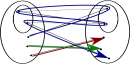
There is an isomorphism in between and .
Proof 5.7.
By definition of the interpretation of types, this boils down to an isomorphism in between the two arenas and represented in Figure 10. Informally, the left-to-right isomorphism can be described as follows:
As long as no has been played, it behaves as the identity. The first time a is played, Player copies it on the right side. One can then check that the play has possible extensions on the left hand side, whereas it only has extensions on the right hand side. Therefore, Player has to fix a bijection and play accordingly. In general if occurrences of have been played, there are s available on the left hand side and still on the right hand side, therefore Player has to follow a bijection .
Thus there is in fact an infinity of different isomorphisms between and , one for each family of bijections between and .
We note that the strategy from to is visible, so this also gives an example of a morphism in which is not invertible in but becomes invertible in . These strategies are not compact so the definability theorem does not apply, however we can nonetheless manually extract corresponding programs from them. We display them in Figure 11, where we suppose that a family of bijections has already been defined. Unfortunately, these terms are too complex to hope for a reasonably-sized direct proof that their interpretations give the strategies described above or even that they form an isomorphism. This kind of difficulty emphasizes the need for new algebraic methods to manipulate and prove properties of imperative higher-order programs.
It seems difficult to characterize exactly the new isomorphisms that natural numbers allow to define. One can prove that the types and are isomorphic, showing that isomorphisms are non-local. Even worse, replacing any occurrence of by in the types above yields non-isomorphic types. Likewise, and are not isomorphic.
It is also interesting to note that composing with provides an isomorphism , even though curryfication is not a valid isomorphism in general. However one should keep in mind that the terms realizing this isomorphism have nothing in common with curryfication, as they have to use higher-order references in a non-trivial way. In particular, it seems unlikely that they can be used for modularity purposes, putting some limits to the idea that isomorphisms of types always provide the good notion of equivalence on which programmers should rely.
6. Conclusion
We solved Laurent’s conjecture and characterized the isomorphisms of types in . Surprisingly, we realized that the combination of higher-order references, natural numbers and call-by-value allowed to define new non-trivial type isomorphisms. Note however that if well-bracketing is satisfied, the proof of our core game-theoretic theorem adapts directly to arenas where all moves only enable a finite number of questions, but an arbitrary numbers of answers. As a consequence, there are no non-trivial isomorphisms (i.e. not already present in the -calculus) in the call-by-name variant of , although we can define one using call/cc.
Note that despite the seemingly restricted power of , our theorem does apply to all real-life programming languages that have a bounded type of integer, such as or : in this setting, no non-trivial isomorphism can exist. However unbounded natural numbers can be defined using recursive types, so the isomorphism above can be implemented in a call-by-value programming language with recursive types and general references, such as Ocaml.
Acknowledgments. We would like to thank Guy McCusker and Nikos Tzevelekos for stimulating discussions about the new non-trivial isomorphisms.
References
- [1] S. Abramsky, K. Honda, and G. McCusker. A fully abstract game semantics for general references. In 13th IEEE Symposium on Logic in Computer Science. IEEE Computer Society Press, 1998.
- [2] S. Abramsky and G. McCusker. Linearity, Sharing and State: a Fully Abstract Game Semantics for Idealized Algol with active expressions, 1997.
- [3] S. Abramsky and G. McCusker. Call-by-value games. In Mogens Nielsen and Wolfgang Thomas, editors, 6th Annual Conference of the European Association for Computer Science Logic, volume 1414 of Lecture Notes in Computer Science. Springer, 1998.
- [4] F. Atanassow and J. Jeuring. Inferring type isomorphisms generically. In Dexter Kozen and Carron Shankland, editors, MPC, volume 3125 of Lecture Notes in Computer Science, pages 32–53. Springer, 2004.
- [5] G. Barthe and O. Pons. Type isomorphisms and proof reuse in dependent type theory. In Furio Honsell and Marino Miculan, editors, FoSSaCS, volume 2030 of Lecture Notes in Computer Science, pages 57–71. Springer, 2001.
- [6] G. Berry and P.-L. Curien. Sequential algorithms on concrete data structures. Theoretical Computer Science, 20:265–321, 1982.
- [7] K.B. Bruce, R. Di Cosmo, and G. Longo. Provable isomorphisms of types. Mathematical Structures in Computer Science, 2(2):231–247, 1992.
- [8] K.B. Bruce and G. Longo. Provable isomorphisms and domain equations in models of typed languages (preliminary version). In STOC, pages 263–272. ACM, 1985.
- [9] M. Dezani-Ciancaglini. Characterization of normal forms possessing inverse in the ---calculus. Theoretical Computer Science, 2(3):323–337, 1976.
- [10] R. Di Cosmo. Invertibility of terms and valid isomorphisms, a proof theoretic study on second order lambda-calculus with surjective pairing and terminal object. Technical report, Technical Report TR 10-91, LIENS Ecole Normale Supérieure, Paris, 1991.
- [11] R. Di Cosmo. A short survey of isomorphisms of types. Mathematical Structures in Computer Science, 15(5):825–838, 2005.
- [12] M. Fiore, R. Di Cosmo, and V. Balat. Remarks on isomorphisms in typed lambda calculi with empty and sum types. Ann. Pure Appl. Logic, 141(1-2):35–50, 2006.
- [13] K. Honda and N. Yoshida. Game-theoretic analysis of call-by-value computation. Theor. Comput. Sci., 221(1-2):393–456, 1999.
- [14] J.M.E. Hyland and C.H.L. Ong. On full abstraction for PCF: I, II and III. Information and Computation, 163(2):285–408, December 2000.
- [15] J.M.E. Hyland and A. Schalk. Games on graphs and sequentially realizable functionals. In Logic in Computer Science 02, pages 257–264, Kopenhavn, July 2002. IEEE Computer Society Press.
- [16] A. Joyal, R. Street, and D. Verity. Traced monoidal categories. Mathematical Proceedings of the Cambridge Philosophical Society, 119(447-468):184, 1996.
- [17] J. Laird. Full abstraction for functional languages with control. In 12th IEEE Symposium on Logic in Computer Science, pages 58–67, 1997.
- [18] J. Laird. A game semantics of the asynchronous -calculus. In CONCUR, pages 51–65, 2005.
- [19] O. Laurent. Polarized games. Annals of Pure and Applied Logic, 130(1-3):79–123, 2004.
- [20] O. Laurent. Classical isomorphisms of types. Mathematical Structures in Computer Science, 15(5):969–1004, 2005.
- [21] G. McCusker. Games and full abstraction for a functional metalanguage with recursive types. PhD thesis, Imperial College, University of London, 1996. Published in Springer-Verlag’s Distinguished Dissertations in Computer Science series, 1998.
- [22] P.-A. Melliès and N. Tabareau. An algebraic account of references in game semantics. Electr. Notes Theor. Comput. Sci., 249:377–405, 2009.
- [23] E. Moggi. Notions of computation and monads. Information and Computation, 93:55–92, 1991.
- [24] A. Murawski and N. Tzevelekos. Full Abstraction for Reduced ML. In Luca de Alfaro, editor, FOSSACS, volume 5504 of Lecture Notes in Computer Science, pages 32–47. Springer, 2009.
- [25] A. Murawski and N. Tzevelekos. Game semantics for good general references. In LICS, pages 75–84. IEEE Computer Society, 2011.
- [26] M. Rittri. Using types as search keys in function libraries. J. Funct. Program., 1(1):71–89, 1991.
- [27] M. Rittri. Retrieving library functions by unifying types modulo linear isomorphism. ITA, 27(6):523–540, 1993.