Vanishingly Sparse Matrices and Expander Graphs,
With Application to Compressed Sensing

Bubacarr  Bah, and  Jared  Tanner Laboratory for Information and Inference Systems (LIONS), École Polytechnique Fédérale de Lausanne (EPFL), Lausanne, Switzerland (bubacarr.bah@epfl.ch).Mathematics Institute and Exeter College, University of Oxford, Oxford, UK (tanner@maths.ox.ac.uk). J.T. acknowledges support from the Leverhulme Trust.Copyright (c) 2012 IEEE
Abstract

We revisit the probabilistic construction of sparse random matrices where each column has a fixed number of nonzeros whose row indices are drawn uniformly at random with replacement. These matrices have a one-to-one correspondence with the adjacency matrices of fixed left degree expander graphs. We present formulae for the expected cardinality of the set of neighbors for these graphs, and present tail bounds on the probability that this cardinality will be less than the expected value. Deducible from these bounds are similar bounds for the expansion of the graph which is of interest in many applications. These bounds are derived through a more detailed analysis of collisions in unions of sets. Key to this analysis is a novel dyadic splitting technique. The analysis led to the derivation of better order constants that allow for quantitative theorems on existence of lossless expander graphs and hence the sparse random matrices we consider and also quantitative compressed sensing sampling theorems when using sparse non mean-zero measurement matrices.

Index Terms:
Algorithms, compressed sensing, signal processing, sparse matrices, expander graphs.

I Introduction

Sparse matrices are particularly useful in applied and computational mathematics because of their low storage complexity and fast implementation as compared to dense matrices, see [1, 2, 3]. Of late, significant progress has been made to incorporate sparse matrices in compressed sensing, with [4, 5, 6, 7] giving both theoretical performance guarantees and also exhibiting numerical results that shows sparse matrices coming from expander graphs can be as good sensing matrices as their dense counterparts. In fact, Blanchard and Tanner [8] recently demonstrated in a GPU implementation how well these type of matrices do compared to dense Gaussian and Discrete Cosine Transform matrices even with very small fixed number of nonzeros per column (as considered here).

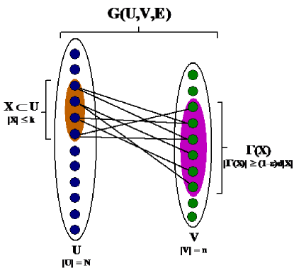
In this manuscript we consider random sparse matrices that are adjacency matrices of lossless expander graphs. Expander graphs are highly connected graphs with very sparse adjacency matrices, a precise definition of a lossless expander graph is given in Definition I.1 and their illustration in Fig. 1.

Definition I.1

G=(U,V,E)𝐺𝑈𝑉𝐸G=\left(U,V,E\right) is a lossless (k,d,ϵ)𝑘𝑑italic-ϵ(k,d,\epsilon)-expander if it is a bipartite graph with |U|=N𝑈𝑁|U|=N left vertices, |V|=n𝑉𝑛|V|=n right vertices and has a regular left degree d𝑑d, such that any XU𝑋𝑈X\subset U with |X|k𝑋𝑘|X|\leq k has |Γ(X)|=(1ϵ)d|X|Γ𝑋1italic-ϵ𝑑𝑋|\Gamma(X)|=\left(1-\epsilon\right)d|X| neighbors. 111Lossless expanders with parameters d,k,n,N𝑑𝑘𝑛𝑁d,k,n,N are equivalent to lossless conductors with parameters that are base 2 logarithms of the parameters of lossless expanders see [9, 5] and the references therein.

Remark I.2
  1. 1.

    The graphs are lossless because ϵ1much-less-thanitalic-ϵ1\epsilon\ll 1;

  2. 2.

    They are called unbalanced expanders when nNmuch-less-than𝑛𝑁n\ll N;

  3. 3.

    The expansion of a lossless (k,d,ϵ)𝑘𝑑italic-ϵ(k,d,\epsilon)-expander graph is (1ϵ)d1italic-ϵ𝑑\left(1-\epsilon\right)d.

Refer to caption
Figure 1: Illustration of a lossless (k,d,ϵ)𝑘𝑑italic-ϵ(k,d,\epsilon)-expander graphs with k=4𝑘4k=4 and d=2𝑑2d=2.

Such graphs have been well studied in theoretical computer science and pure mathematics and have many applications including: Distributed Routing in Networks, Linear Time Decodable Error-Correcting Codes, Bitprobe Complexity of Storing Subsets, Fault-tolerance and a Distributed Storage Method, and Hard Tautologies in Proof Complexity, see [10] or [9] for a more detailed survey. Pinsker and Bassylago [11] proved the existence of lossless expanders and showed that any random left-regular bipartite graph is, with high probability, an expander graph. Probabilistic constructions with optimal parameters n,N𝑛𝑁n,N exist but are not suitable for the applications we consider here. Deterministic constructions only achieve sub-optimal parameters, see Guruswami et. al. [12].

Our main contribution, is the presentation of quantitative guarantees on the probabilistic construction of these objects in the form of a bound on the tail probability of the size of the set of neighbors, Γ(X)Γ𝑋\Gamma(X) for a given XU𝑋𝑈X\subset U, of a randomly generated left-degree bipartite graph. Moreover, we provide deducible bounds on the tail probability of the expansion of the graph, |Γ(X)|/|X|Γ𝑋𝑋|\Gamma(X)|/|X|. We derive quantitative guarantees for randomly generated non-mean zero sparse binary matrices to be adjacency matrices of expander graphs. In addition, we derive the first phase transitions showing regions in parameter space that depict when a left-regular bipartite graph with a given set of parameters is guaranteed to be a lossless expander with high probability. The most significant contribution, which is the key innovation, of this paper is the use of a novel technique of dyadic splitting of sets. We derived our bounds using this technique and apply them to derive 1subscript1\ell_{1} restricted isometry constants (RIC1subscriptRIC1\mathrm{RIC}_{1}).

Numerous compressed sensing algorithms have been designed for sparse matrices [4, 5, 6, 7]. Another contribution of our work is the derivation of sampling theorems, presented as phase transitions, comparing performance guarantees for some of these algorithms as well as the more traditional 1subscript1\ell_{1} minimization compressed sensing formulation. We also show how favorably 1subscript1\ell_{1} minimization performance guarantees for such sparse matrices compared to what 2subscript2\ell_{2} restricted isometry constants (RIC2subscriptRIC2\mathrm{RIC}_{2}) analysis yields for the dense Gaussian matrices. For this comparison, we used sampling theorems and phase transitions from related work by Blanchard et. al. [13] that provided such theorems for dense Gaussian matrices based on RIC2subscriptRIC2\mathrm{RIC}_{2} analysis.

The outline of the rest of this introduction section goes as follows. In Section I-A we present our main results in Theorem I.6 and Corollary I.7. In Section I-B we discuss RIC1subscriptRIC1\mathrm{RIC}_{1} and its implication for compressed sensing, leading to two sampling theorems in Corollaries I.10 and I.11.

I-A Main results

Our main results is about a class of sparse matrices coming from lossless expander graphs, a class which include non-mean zero matrices. We start by defining the class of matrices we consider and a key concept of a set of neighbors used in the derivation of the main results of the manuscript. Firstly, we denote H(p):=plog(p)(1p)log(1p)assignH𝑝𝑝𝑝1𝑝1𝑝\hbox{H}(p):=-p\log(p)-(1-p)\log(1-p) as the Shannon entropy function of base e𝑒e logarithm.

Definition I.3

Let A𝐴A be an n×N𝑛𝑁n\times N matrix with d𝑑d nonzeros in each column. We refer to A𝐴A as a random

  1. 1.

    sparse expander (SE) if every nonzero has value 111

  2. 2.

    sparse signed expander (SSE) if every nonzero has value from {1,1}11\{-1,1\}

and the support set of the d𝑑d nonzeros per column are drawn uniformly at random, with each column drawn independently.

SE matrices are adjacency matrices of lossless (k,d,ϵ)𝑘𝑑italic-ϵ(k,d,\epsilon)-expander graphs while SSE matrices have random sign patterns in the nonzeros of an adjacency matrix of a lossless (k,d,ϵ)𝑘𝑑italic-ϵ(k,d,\epsilon)-expander graph. If A𝐴A is either an SE or SSE it will have only d𝑑d nonzeros per column and since we fix dnmuch-less-than𝑑𝑛d\ll n, A𝐴A is therefore “vanishingly sparse.” We denote ASsubscript𝐴𝑆A_{S} as a submatrix of A𝐴A composed of columns of A𝐴A indexed by the set S𝑆S with |S|=s𝑆𝑠|S|=s. To aid translation between the terminology of graph theory and linear algebra we define the set of neighbors in both notation.

Definition I.4

Consider a bipartite graph G=(U,V,E)𝐺𝑈𝑉𝐸G=(U,V,E) where E𝐸E is the set of edges and eij=(xi,yj)subscript𝑒𝑖𝑗subscript𝑥𝑖subscript𝑦𝑗e_{ij}=(x_{i},y_{j}) is the edge that connects vertex xisubscript𝑥𝑖x_{i} to vertex yjsubscript𝑦𝑗y_{j}. For a set of left vertices SU𝑆𝑈S\subset U its set of neighbors is Γ(S)={yj|xiS and eijE}Γ𝑆conditional-setsubscript𝑦𝑗subscript𝑥𝑖𝑆 and subscript𝑒𝑖𝑗𝐸\Gamma(S)=\{y_{j}|x_{i}\in S\mbox{ and }e_{ij}\in E\}. In terms of the adjacency matrix, A𝐴A, of G=(U,V,E)𝐺𝑈𝑉𝐸G=(U,V,E) the set of neighbors of ASsubscript𝐴𝑆A_{S} for |S|=s𝑆𝑠|S|=s, denoted by Assubscript𝐴𝑠A_{s}, is the set of rows with at least one nonzero.

Definition I.5

Using Definition I.4 the expansion of the graph is given by the ratio |Γ(S)|/|S|Γ𝑆𝑆|\Gamma(S)|/|S|, or equivalently, |As|/ssubscript𝐴𝑠𝑠|A_{s}|/s.

By the definition of a lossless expander, Definition I.1, we need |Γ(S)|Γ𝑆\left|\Gamma(S)\right| to be large for every small SU𝑆𝑈S\subset U. In terms of the class of matrices defined by Definition I.3, for every ASsubscript𝐴𝑆A_{S} we want to have |As|subscript𝐴𝑠|A_{s}| as close to n𝑛n as possible, where n𝑛n is the number of rows. Henceforth, we will only use the linear algebra notation Assubscript𝐴𝑠A_{s} which is equivalent to Γ(S)Γ𝑆\Gamma(S). Note that |As|subscript𝐴𝑠\left|A_{s}\right| is a random variable depending on the draw of the set of columns, S𝑆S, for each fixed A𝐴A. Therefore, we can ask what is the probability that |As|subscript𝐴𝑠\left|A_{s}\right| is not greater than assubscript𝑎𝑠a_{s}, in particular where assubscript𝑎𝑠a_{s} is smaller than the expected value of |As|subscript𝐴𝑠\left|A_{s}\right|. This is the question that Theorem I.6 to answers. We then use this theorem with RIC1subscriptRIC1\mathrm{RIC}_{1} to deduce the corollaries that follow which are about the probabilistic construction of expander graphs, the matrices we consider, and sampling theorems of some selected compressed sensing algorithms.

Theorem I.6

For fixed s,n,N𝑠𝑛𝑁s,n,N and d𝑑d, let an n×N𝑛𝑁n\times N matrix, A𝐴A be drawn from either of the classes of matrices defined in Definition I.3, then

Prob(|As|as)<pmax(s,d)×exp[nΨ(as,,a1)]Probsubscript𝐴𝑠subscript𝑎𝑠subscript𝑝𝑚𝑎𝑥𝑠𝑑𝑛Ψsubscript𝑎𝑠subscript𝑎1\hbox{Prob}\left(\left|A_{s}\right|\leq a_{s}\right)<p_{max}(s,d)\\ \times\exp\left[n\cdot\Psi\left(a_{s},\ldots,a_{1}\right)\right] (1)

where pmax(s,d)subscript𝑝𝑚𝑎𝑥𝑠𝑑p_{max}(s,d) is given by

pmax(s,d)=2252πs3d3,andsubscript𝑝𝑚𝑎𝑥𝑠𝑑2252𝜋superscript𝑠3superscript𝑑3andp_{max}(s,d)=\frac{2}{25\sqrt{2\pi s^{3}d^{3}}},\qquad\mbox{and} (2)
Ψ(as,,a1)=1n[i=1s/2s2i((nai)H(a2iainai)+aiH(a2iaiai)nH(ain))+3slog(5d)]Ψsubscript𝑎𝑠subscript𝑎11𝑛delimited-[]superscriptsubscript𝑖1𝑠2𝑠2𝑖𝑛subscript𝑎𝑖Hsubscript𝑎2𝑖subscript𝑎𝑖𝑛subscript𝑎𝑖subscript𝑎𝑖Hsubscript𝑎2𝑖subscript𝑎𝑖subscript𝑎𝑖𝑛Hsubscript𝑎𝑖𝑛3𝑠5𝑑\Psi\left(a_{s},\ldots,a_{1}\right)=\frac{1}{n}\Bigg{[}\sum_{i=1}^{\lceil s/2\rceil}\frac{s}{2i}\left(\left(n-a_{i}\right)\cdot\hbox{H}\left(\frac{a_{2i}-a_{i}}{n-a_{i}}\right)\right.\\ \left.+a_{i}\cdot\hbox{H}\left(\frac{a_{2i}-a_{i}}{a_{i}}\right)-n\cdot\hbox{H}\left(\frac{a_{i}}{n}\right)\right)+3s\log\left(5d\right)\Bigg{]} (3)

where a1:=dassignsubscript𝑎1𝑑a_{1}:=d.

If no restriction is imposed on assubscript𝑎𝑠a_{s} then the aisubscript𝑎𝑖a_{i} for i>1𝑖1i>1 take on their expected value a^isubscript^𝑎𝑖\widehat{a}_{i} given by

a^2i=a^i(2a^in)fori=1,2,4,,s/2.formulae-sequencesubscript^𝑎2𝑖subscript^𝑎𝑖2subscript^𝑎𝑖𝑛for𝑖124𝑠2\displaystyle\widehat{a}_{2i}=\widehat{a}_{i}\left(2-\frac{\widehat{a}_{i}}{n}\right)\quad\mbox{for}\quad i=1,2,4,\ldots,\lceil s/2\rceil. (4)

If assubscript𝑎𝑠a_{s} is restricted to be less than a^ssubscript^𝑎𝑠\widehat{a}_{s}, then the aisubscript𝑎𝑖a_{i} for i>1𝑖1i>1 are the unique solutions to the following polynomial system

a2i32aia2i2+2ai2a2iai2a4i=0for i=1,2,,s/4formulae-sequencesuperscriptsubscript𝑎2𝑖32subscript𝑎𝑖superscriptsubscript𝑎2𝑖22superscriptsubscript𝑎𝑖2subscript𝑎2𝑖superscriptsubscript𝑎𝑖2subscript𝑎4𝑖0for 𝑖12𝑠4a_{2i}^{3}-2a_{i}a_{2i}^{2}+2a_{i}^{2}a_{2i}-a_{i}^{2}a_{4i}=0~{}\mbox{for }~{}i=1,2,\ldots,\lceil s/4\rceil (5)

with a2iaisubscript𝑎2𝑖subscript𝑎𝑖a_{2i}\geq a_{i} for each i𝑖i.

Corollary I.7

For fixed s,n,N,d𝑠𝑛𝑁𝑑s,n,N,d and 0<ϵ<1/20italic-ϵ120<\epsilon<1/2, let an n×N𝑛𝑁n\times N matrix, A𝐴A be drawn from the class of matrices defined in Definition I.3, then

Prob(ASx1(12ϵ)dx1)<pmax(s,d)×exp[nΨ(s,d,ϵ)]Probsubscriptnormsubscript𝐴𝑆𝑥112italic-ϵ𝑑subscriptdelimited-∥∥𝑥1subscript𝑝𝑚𝑎𝑥𝑠𝑑𝑛Ψ𝑠𝑑italic-ϵ\hbox{Prob}\left(\mathop{\|A_{S}x\|_{1}}\leq(1-2\epsilon)d\|x\|_{1}\right)<p_{max}(s,d)\\ \times\exp\left[n\cdot\Psi\left(s,d,\epsilon\right)\right] (6)

where Ψ(s,d,ϵ)=Ψ(as,,a1)Ψ𝑠𝑑italic-ϵΨsubscript𝑎𝑠subscript𝑎1\Psi\left(s,d,\epsilon\right)=\Psi\left(a_{s},\ldots,a_{1}\right) in (3) with as=(1ϵ)dssubscript𝑎𝑠1italic-ϵ𝑑𝑠a_{s}=(1-\epsilon)ds and a1=dsubscript𝑎1𝑑a_{1}=d, and pmax(s,d)subscript𝑝𝑚𝑎𝑥𝑠𝑑p_{max}(s,d) is the polynomial in (2).

Theorem I.6 and Corollary I.7 allow us to calculate s,n,N,d,ϵ𝑠𝑛𝑁𝑑italic-ϵs,n,N,d,\epsilon where the probability of the probabilistic constructions in Definition I.3 not being a lossless (s,d,ϵ)𝑠𝑑italic-ϵ(s,d,\epsilon)-expander is exponentially small. For moderate values of ϵitalic-ϵ\epsilon this allows us to make quantitative sampling theorems for some compressed sensing reconstruction algorithms.

I-B RIC1subscriptRIC1\mathrm{RIC}_{1} and its implications to Compressed Sensing

In compressed sensing, and by extension in sparse approximation, we observe the effect of the application of a matrix to a vector of interest and we endeavor to recovery this vector of interest by exploiting the inherent simplicity in this vector. Precisely, let xN,𝑥superscript𝑁x\in\mathbb{R}^{N}, be the vector of interest whose simplicity is that it has k<N𝑘𝑁k<N nonzeros, which we refer to as klimit-from𝑘k-sparse; then we observe yn,𝑦superscript𝑛y\in\mathbb{R}^{n}, as the measurement vector resulting from the multiplication of x𝑥x by an n×N𝑛𝑁{n\times N} matrix, A𝐴A. The minimum simplicity reconstruct of x𝑥x can be written as

minxχNx0subject toAx=y,subscript𝑥superscript𝜒𝑁subscriptnorm𝑥0subject to𝐴𝑥𝑦\min_{x\in\chi^{N}}\|x\|_{0}\quad\mbox{subject to}\quad Ax=y, (7)

where χNsuperscript𝜒𝑁\chi^{N} is the set of all klimit-from𝑘k-sparse vectors and z0subscriptnorm𝑧0\|z\|_{0} counts the nonzero components of z𝑧z; this model may be reformulated to include noise in the measurements. References [14, 15, 16, 17] give detailed introductions to compressed sensing and its applications; while [18, 19, 20, 21, 22, 5, 6, 23, 4, 24] provide information on some of the popular computationally efficient algorithms used to solve problem (7) and its reformulations.

We are able to give guarantees on the quality of the reconstructed vector from A𝐴A and y𝑦y from a variety of reconstruction algorithms. One of these guarantees is a bound on the approximation error between our recovered vector, say x^^𝑥\hat{x}, and the original vector by the best k𝑘k-term representation error i.e. xx^1Const.xxk1formulae-sequencesubscriptnorm𝑥^𝑥1𝐶𝑜𝑛𝑠𝑡subscriptnorm𝑥subscript𝑥𝑘1\|x-\hat{x}\|_{1}\leq Const.\|x-x_{k}\|_{1} where xksubscript𝑥𝑘x_{k} is the optimal k𝑘k-term representation for x𝑥x. This is possible if A𝐴A has small RIC1subscriptRIC1\mathrm{RIC}_{1}, in other words A𝐴A satisfies the 1subscript1\ell_{1} restricted isometry property (RIP-1), introduced by Berinde et. al. in [5] and defined as thus.

Definition I.8 (RIP-1)

Let χNsuperscript𝜒𝑁\chi^{N} be the set of all klimit-from𝑘k-sparse vectors, then an n×N𝑛𝑁n\times N matrix A𝐴A has RIP-1, with the lower RIC1subscriptRIC1\mathrm{RIC}_{1} being the smallest L(k,n,N;A)𝐿𝑘𝑛𝑁𝐴L(k,n,N;A), when the following condition holds.

(1L(k,n,N;A))x1Ax1x1xχN.1𝐿𝑘𝑛𝑁𝐴subscriptnorm𝑥1subscriptnorm𝐴𝑥1subscriptnorm𝑥1for-all𝑥superscript𝜒𝑁\left(1-L(k,n,N;A)\right)||x||_{1}\leq||Ax||_{1}\leq||x||_{1}~{}~{}\forall x\in\chi^{N}. (8)

For computational purposes it is preferable to have A𝐴A sparse, but little quantitative information on L(k,n,N;A)𝐿𝑘𝑛𝑁𝐴L(k,n,N;A) has been available for large sparse rectangular matrices. Berinde et. al. in [5] showed that scaled adjacency matrices of lossless expander graphs (i.e. scaled SE matrices) satisfy RIP-1, and the same proof extends to the signed adjacency matrices (i.e. so called SSE matrices).

Theorem I.9

If an n×N𝑛𝑁n\times N matrix A𝐴A is either SE or SSE defined in Definition I.3, then A/d𝐴𝑑A/d satisfies RIP-1 with L(k,n,N;A)=2ϵ𝐿𝑘𝑛𝑁𝐴2italic-ϵL(k,n,N;A)=2\epsilon.

Proof:

The proof of the signed case (SSE) follows that of the unsigned case (SE) in [5] but with absolute values included in the appropriate stages. ∎

Based on Theorem I.9 which guarantees RIP-1, (8), for the class of matrices in Definition I.3, we give a bound, in Corollary I.10, for the probability that a random draw of a matrix with d1𝑑1d~{}1s or ±1plus-or-minus1\pm 1s in each column fails to satisfy the lower bound of RIP-1 and hence fails to come from the class of matrices given in Definition I.3. In addition to Theorem I.9, Corollary I.10 follows from Theorem I.6 and Corollary I.7.

Corollary I.10

Considering RIP-1, if A𝐴A is drawn from the class of matrices in Definition I.3 and 0<ϵ<1/20italic-ϵ120<\epsilon<1/2 with k,n,N𝑘𝑛𝑁k,n,N fixed, then for all k𝑘k-sparse vectors x𝑥x

Prob(Ax1(12ϵ)dx1)<pmax(N,k,d)×exp[NΨnet(k,n,N;d,ϵ)]Probsubscriptdelimited-∥∥𝐴𝑥112italic-ϵ𝑑subscriptdelimited-∥∥𝑥1subscriptsuperscript𝑝𝑚𝑎𝑥𝑁𝑘𝑑𝑁subscriptΨ𝑛𝑒𝑡𝑘𝑛𝑁𝑑italic-ϵ\hbox{Prob}\left(\|Ax\|_{1}\leq(1-2\epsilon)d\|x\|_{1}\right)<p^{\prime}_{max}(N,k,d)\\ \times\exp\left[N\cdot\Psi_{net}\left(k,n,N;d,\epsilon\right)\right] (9)

where pmax(N,k,d)subscriptsuperscript𝑝𝑚𝑎𝑥𝑁𝑘𝑑p^{\prime}_{max}(N,k,d) and ΨnetsubscriptΨ𝑛𝑒𝑡\Psi_{net} are given by

pmax(N,k,d)subscriptsuperscript𝑝𝑚𝑎𝑥𝑁𝑘𝑑\displaystyle p^{\prime}_{max}(N,k,d) =116πkd3(1kN),absent116𝜋𝑘superscript𝑑31𝑘𝑁\displaystyle=\frac{1}{16\pi k\sqrt{d^{3}\left(1-\frac{k}{N}\right)}}, (10)
Ψnet(k,n,N;d,ϵ)subscriptΨ𝑛𝑒𝑡𝑘𝑛𝑁𝑑italic-ϵ\displaystyle\Psi_{net}\left(k,n,N;d,\epsilon\right) =H(kN)+nNΨ(k,d,ϵ),absentH𝑘𝑁𝑛𝑁Ψ𝑘𝑑italic-ϵ\displaystyle=\hbox{H}\left(\frac{k}{N}\right)+\frac{n}{N}\Psi\left(k,d,\epsilon\right), (11)

with Ψ(k,d,ϵ)Ψ𝑘𝑑italic-ϵ\Psi\left(k,d,\epsilon\right) defined in Corollary I.7.

Furthermore, the following corollary is a consequence of Corollary I.10 and it is a sampling theorem on the existence of lossless expander graphs. The proof of Corollaries I.10 and I.11 are presented in Sections IV-B2 and IV-B3 respectively.

Corollary I.11

Consider 0<ϵ<1/20italic-ϵ120<\epsilon<1/2 and d𝑑d fixed. If A𝐴A is drawn from the class of matrices in Definition I.3 and all x𝑥x drawn from χNsuperscript𝜒𝑁\chi^{N} with (k,n,N)𝑘𝑛𝑁(k,n,N)\rightarrow\infty while k/nρ(0,1)𝑘𝑛𝜌01k/n\rightarrow\rho\in(0,1) and n/Nδ(0,1)𝑛𝑁𝛿01n/N\rightarrow\delta\in(0,1) then for ρ<(1γ)ρexp(δ;d,ϵ)𝜌1𝛾superscript𝜌𝑒𝑥𝑝𝛿𝑑italic-ϵ\rho<(1-\gamma)\rho^{exp}(\delta;d,\epsilon) and γ>0𝛾0\gamma>0

Prob(Ax1(12ϵ)dx1)1Probsubscriptnorm𝐴𝑥112italic-ϵ𝑑subscriptnorm𝑥11\hbox{Prob}\left(\|Ax\|_{1}\geq(1-2\epsilon)d\|x\|_{1}\right)\rightarrow 1 (12)

exponentially in n𝑛n, where ρexp(δ;d,ϵ)superscript𝜌𝑒𝑥𝑝𝛿𝑑italic-ϵ\rho^{exp}(\delta;d,\epsilon) is the largest limiting value of k/n𝑘𝑛k/n for which

H(kN)+nNΨ(k,d,ϵ)=0.H𝑘𝑁𝑛𝑁Ψ𝑘𝑑italic-ϵ0\hbox{H}\left(\frac{k}{N}\right)+\frac{n}{N}\Psi\left(k,d,\epsilon\right)=0. (13)

The outline of the rest of the manuscript is as follows: In Section II we show empirical data to validate our main results and also present lemmas (and their proofs) that are key to the proof of the main theorem, Theorem I.6. In Section III we discuss restricted isometry constants and compressed sensing algorithms. In Section IV we prove the mains results, that is Theorem I.6 and the corollaries in Sections I-A and I-B. Section V is the appendix where we present the alternative to Theorem I.6.

II Discussion and derivation of the main results

We present the method used to derive the main results and discuss the validity and implications of the method. We start by presenting in the next subsection, Section II-A, numerical results that support the claims of the main results in Sections I-A and I-B. This is followed in Section II with lemmas, propositions and corollaries and their proofs.

II-A Discussion on main results

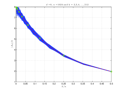
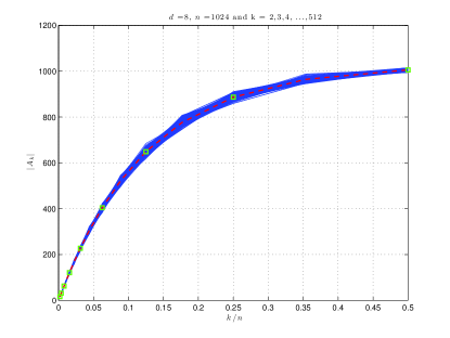
Theorem I.6 gives a bound on the probability that the cardinality of a union of k𝑘k sets each with d𝑑d elements, i.e. |Ak|subscript𝐴𝑘|A_{k}|, is less than aksubscript𝑎𝑘a_{k}. Fig. 2 shows plots of values of |Ak|subscript𝐴𝑘|A_{k}| (size of set of neighbors) for different k𝑘k (in blue), superimposed on these plots is the mean value of |Ak|subscript𝐴𝑘|A_{k}| (in red) both taken over 500 realizations and the a^ksubscript^𝑎𝑘\widehat{a}_{k} in green. Similarly, Fig. 3 also shows values of |Ak|/ksubscript𝐴𝑘𝑘|A_{k}|/k (the graph expansion) also taken over 500 realizations.
Refer to caption
Figure 2: For fixed d=8𝑑8d=8 and n=210𝑛superscript210n=2^{10}, over 500500500 realizations we plot (in blue) the cardinalities of the index sets of nonzeros in a given number of set sizes, k𝑘k. The dotted red curve is mean of the simulations and the green squares are the a^ksubscript^𝑎𝑘\hat{a}_{k}.
Refer to caption
Figure 3: For fixed d=8𝑑8d=8 and n=210𝑛superscript210n=2^{10}, over 500500500 realizations we plot (in blue) the graph expansion for a given input set size k𝑘k. The dotted red curve is mean of the simulations and the green squares are the a^k/ksubscript^𝑎𝑘𝑘\hat{a}_{k}/k.

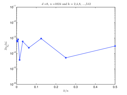
Theorem I.6 also claims that the a^ssubscript^𝑎𝑠\hat{a}_{s} are the expected values of the cardinalities of the union of s𝑠s sets. We give a brief sketch of its proof in Section II-B in terms of the maximum likelihood and empirical illustrate the accuracy of the result in Fig. 4 where we show the relative error between a^ksubscript^𝑎𝑘\hat{a}_{k} and the mean values of the ak,a¯ksubscript𝑎𝑘subscript¯𝑎𝑘a_{k},\bar{a}_{k}, realized over 500500500 runs, to be less than 103superscript10310^{-3}.

Refer to caption
Figure 4: For fixed d=8𝑑8d=8 and n=210𝑛superscript210n=2^{10}, over 500500500 realizations the relative error between the mean values of aksubscript𝑎𝑘a_{k} (referred to as a¯ksubscript¯𝑎𝑘\bar{a}_{k}) and the a^ksubscript^𝑎𝑘\hat{a}_{k} from Equation (4) of Theorem I.6.
Refer to caption
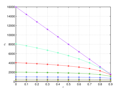
Figure 5: Values of aisubscript𝑎𝑖a_{i}as a function of ϵ[0,1)italic-ϵ01\epsilon\in[0,1) for ak:=(1ϵ)a^kassignsubscript𝑎𝑘1italic-ϵsubscript^𝑎𝑘a_{k}:=(1-\epsilon)\hat{a}_{k} with d=8𝑑8d=8, k=2×10³𝑘2superscript103k=2\times 10^{3} and n=220𝑛superscript220n=2^{20}. For this choice of d,k,n𝑑𝑘𝑛d,k,n there are twelve levels of dyadic splits resulting in aisubscript𝑎𝑖a_{i} for i=2j𝑖superscript2𝑗i=2^{j} for j=0,,log2k=12formulae-sequence𝑗0subscript2𝑘12j=0,\ldots,\lceil\log_{2}k\rceil=12. The highest curve corresponds to aisubscript𝑎𝑖a_{i} for i=212𝑖superscript212i=2^{12}, the next highest curve corresponds to i=211𝑖superscript211i=2^{11}, and continuing in decreasing magnitude with decreasing subscript values.

Fig. 5 shows representative values of aisubscript𝑎𝑖a_{i} from (5) for ak:=(1ϵ)a^kassignsubscript𝑎𝑘1italic-ϵsubscript^𝑎𝑘a_{k}:=(1-\epsilon)\hat{a}_{k} as a function of ϵitalic-ϵ\epsilon for d=8𝑑8d=8, k=2×10³𝑘2superscript103k=2\times 10^{3}, and n=220𝑛superscript220n=2^{20}. Each of the aisubscript𝑎𝑖a_{i} decrease smoothly towards d𝑑d, but with aisubscript𝑎𝑖a_{i} for smaller values if i𝑖i varying less than for larger values of i𝑖i.

For fixed 0<ϵ<1/20italic-ϵ120<\epsilon<1/2 and for small but fixed d𝑑d, ρexp(δ;d,ϵ)superscript𝜌𝑒𝑥𝑝𝛿𝑑italic-ϵ\rho^{exp}(\delta;d,\epsilon) in Corollary I.11 is a function of δ𝛿\delta for each d𝑑d and ϵitalic-ϵ\epsilon, is a phase transition function in the (δ,ρ)𝛿𝜌(\delta,\rho) plane. Below the curve of ρexp(δ;d,ϵ)superscript𝜌𝑒𝑥𝑝𝛿𝑑italic-ϵ\rho^{exp}(\delta;d,\epsilon) the probability in (12) goes to one exponentially in n𝑛n as the problem size grows. That is if A𝐴A is drawn at random with d1𝑑1d~{}1s or d±1plus-or-minus𝑑1d~{}\pm 1s in each column and having parameters (k,n,N)𝑘𝑛𝑁(k,n,N) that fall below the curve of ρexp(δ;d,ϵ)superscript𝜌𝑒𝑥𝑝𝛿𝑑italic-ϵ\rho^{exp}(\delta;d,\epsilon) then we say it is from the class of matrices in Definition I.3 with probability approaching one exponentially in n𝑛n. In terms of |Γ(X)|Γ𝑋|\Gamma(X)| for XU𝑋𝑈X\subset U and |X|k𝑋𝑘|X|\leq k, Corollary I.11 say that the probability |Γ(X)|(1ϵ)dkΓ𝑋1italic-ϵ𝑑𝑘|\Gamma(X)|\geq(1-\epsilon)dk goes to one exponentially in n𝑛n if the parameters of our graph lies in the region below ρexp(δ;d,ϵ)superscript𝜌𝑒𝑥𝑝𝛿𝑑italic-ϵ\rho^{exp}(\delta;d,\epsilon). This implies that if we draw a random bipartite graphs that has parameters in the region below the curve of ρexp(δ;d,ϵ)superscript𝜌𝑒𝑥𝑝𝛿𝑑italic-ϵ\rho^{exp}(\delta;d,\epsilon) then with probability approaching one exponentially in n𝑛n that graph is a lossless (k,d,ϵ)𝑘𝑑italic-ϵ(k,d,\epsilon)-expander.

Refer to caption
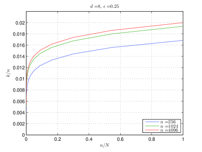
Figure 6: Phase transition plots of ρexp(δ;d,ϵ)superscript𝜌𝑒𝑥𝑝𝛿𝑑italic-ϵ\rho^{exp}(\delta;d,\epsilon) for fixed d=8𝑑8d=8 and ϵ=1/4italic-ϵ14\epsilon=1/4 with n𝑛n varied.

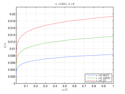
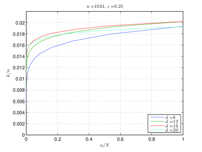
Fig. 6 shows a plot of what ρexp(δ;d,ϵ)superscript𝜌𝑒𝑥𝑝𝛿𝑑italic-ϵ\rho^{exp}(\delta;d,\epsilon) converge to for different values of n𝑛n with ϵitalic-ϵ\epsilon and d𝑑d fixed; Fig. 7 shows a plot of what ρexp(δ;d,ϵ)superscript𝜌𝑒𝑥𝑝𝛿𝑑italic-ϵ\rho^{exp}(\delta;d,\epsilon) converge to for different values of d𝑑d with ϵitalic-ϵ\epsilon and n𝑛n fixed; while Fig. 8 shows plots of what ρexp(δ;d,ϵ)superscript𝜌𝑒𝑥𝑝𝛿𝑑italic-ϵ\rho^{exp}(\delta;d,\epsilon) converge to for different values of ϵitalic-ϵ\epsilon with n𝑛n and d𝑑d fixed. It is interesting to note how increasing d𝑑d increases the phase transition up to a point then it decreases the phase transition. Essentially beyond d=16𝑑16d=16 there is no gain in increasing d𝑑d. This vindicates the use of small d𝑑d in most of the numerical simulations involving the class of matrices considered here. Note the vanishing sparsity as the problem size (k,n,N)𝑘𝑛𝑁(k,n,N) grows while d𝑑d is fixed to a small value of 888. In their GPU implementation [8] Blanchard and Tanner observed that SSE with d=7𝑑7d=7 has a phase transition for numerous sparse approximation algorithms that is consistent with dense Gaussian matrices, but with dramatically faster implementation.
Refer to caption
Figure 7: Phase transition plots of ρexp(δ;d,ϵ)superscript𝜌𝑒𝑥𝑝𝛿𝑑italic-ϵ\rho^{exp}(\delta;d,\epsilon) for fixed ϵ=1/6italic-ϵ16\epsilon=1/6 and n=210𝑛superscript210n=2^{10} with d𝑑d varied.

As afore-stated Corollary I.11 follows from Theorem I.6, alternatively Corollary I.11 can be arrived at based on probabilistic constructions of expander graphs given by Proposition II.1 below. This proposition and its proof can be traced back to Pinsker in [25] but for more recent proofs see [26, 10].

Proposition II.1

For any N/2k1,ϵ>0formulae-sequence𝑁2𝑘1italic-ϵ0N/2\geq k\geq 1,~{}\epsilon>0 there exists a lossless (k,d,ϵ)𝑘𝑑italic-ϵ(k,d,\epsilon)-expander with

d=𝒪(log(N/k)/ϵ)andn=𝒪(klog(N/k)/ϵ2).formulae-sequence𝑑𝒪𝑁𝑘italic-ϵand𝑛𝒪𝑘𝑁𝑘superscriptitalic-ϵ2\displaystyle d=\mathcal{O}\left(\log\left(N/k\right)/\epsilon\right)\quad\mbox{and}\quad n=\mathcal{O}\left(k\log\left(N/k\right)/\epsilon^{2}\right).
Refer to caption
Figure 8: Phase transition plots of ρexp(δ;d,ϵ)superscript𝜌𝑒𝑥𝑝𝛿𝑑italic-ϵ\rho^{exp}(\delta;d,\epsilon) for fixed d=8𝑑8d=8 and n=210𝑛superscript210n=2^{10} with ϵitalic-ϵ\epsilon varied.

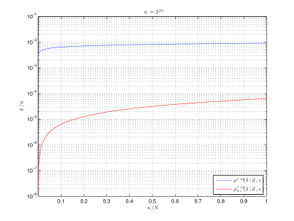
To put our results in perspective, we compare them to the alternative construction in [26] which led to Corollary II.2, whose proof is given in Section V-A of the Appendix. Fig. 9 compares the phase transitions resulting from our construction to that presented in [26], but we must point out however, that the proof in [26] was not aimed for a tight bound.
Refer to caption
Figure 9: A comparison of ρexpsuperscript𝜌𝑒𝑥𝑝\rho^{exp} in Theorem I.6 to ρbiexpsuperscriptsubscript𝜌𝑏𝑖𝑒𝑥𝑝\rho_{bi}^{exp} of Corollary II.2 derived using the construction based on Corollary II.2.
Corollary II.2

Consider a bipartite graph G=(U,V,E)𝐺𝑈𝑉𝐸G=(U,V,E) with left vertices |U|=N𝑈𝑁|U|=N, right vertices |V|=n𝑉𝑛|V|=n and left degree d𝑑d. Fix 0<ϵ<1/20italic-ϵ120<\epsilon<1/2 and d𝑑d, as (k,n,N)𝑘𝑛𝑁(k,n,N)\rightarrow\infty while k/nρ(0,1)𝑘𝑛𝜌01k/n\rightarrow\rho\in(0,1) and n/Nδ(0,1)𝑛𝑁𝛿01n/N\rightarrow\delta\in(0,1) then for ρ<(1γ)ρbiexp(δ;d,ϵ)𝜌1𝛾superscriptsubscript𝜌𝑏𝑖𝑒𝑥𝑝𝛿𝑑italic-ϵ\rho<(1-\gamma)\rho_{bi}^{exp}(\delta;d,\epsilon) and γ>0𝛾0\gamma>0

Prob(Gfails to be an expander)0Prob𝐺fails to be an expander0\hbox{Prob}\left(G~{}\mbox{fails to be an expander}\right)\rightarrow 0 (14)

exponentially in n𝑛n, where ρbiexp(δ;d,ϵ)superscriptsubscript𝜌𝑏𝑖𝑒𝑥𝑝𝛿𝑑italic-ϵ\rho_{bi}^{exp}(\delta;d,\epsilon) is the largest limiting value of k/n𝑘𝑛k/n for which

Ψ(k,n,N;d,ϵ)=0Ψ𝑘𝑛𝑁𝑑italic-ϵ0\Psi\left(k,n,N;d,\epsilon\right)=0 (15)

with Ψ(k,n,N;d,ϵ)=H(kN)+dkNH(ϵ)+ϵdkNlog(dkn)Ψ𝑘𝑛𝑁𝑑italic-ϵH𝑘𝑁𝑑𝑘𝑁Hitalic-ϵitalic-ϵ𝑑𝑘𝑁𝑑𝑘𝑛\displaystyle\Psi\left(k,n,N;d,\epsilon\right)=\mbox{H}\left(\frac{k}{N}\right)+\frac{dk}{N}\mbox{H}\left(\epsilon\right)+\frac{\epsilon dk}{N}\log\left(\frac{dk}{n}\right).

II-B Key Lemmas

The following set of lemmas, propositions and corollaries form the building blocks of the proof of our main results to be presented in Section IV.

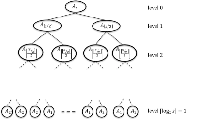
For one fixed set of columns of A𝐴A, denoted ASsubscript𝐴𝑆A_{S}, the probability in (1) can be understood as the cardinality of the unions of nonzeros in the columns of ASsubscript𝐴𝑆A_{S}. Our analysis of this probability follows from a nested unions of subsets using a dyadic splitting technique. Given a starting set of columns we recursively split the number of columns from this set, and the resulting sets, into two sets composed of the ceiling and floor of half of the number of columns of the set we split. In other words, given a starting support set S𝑆S (referred to as the parent set), we split it into two disjoint sets of size s/2𝑠2\lceil s/2\rceil and s/2𝑠2\lfloor s/2\rfloor (referred to as children). Then we union the nonzero elements in the columns indexed by the children sets to get As/2subscript𝐴𝑠2A_{\lceil s/2\rceil} and As/2subscript𝐴𝑠2A_{\lfloor s/2\rfloor}. We continue this process until at a level when the cardinalities in each child set is at most two. Resulting from this type of splitting is a regular binary tree where the size of each child is either the ceiling or the floor of the size of it’s parent set. The root of the binary is our starting set S𝑆S or Assubscript𝐴𝑠A_{s} which we refer to as level 0. Then, the splitting, as described above proceeds till level log21subscript21\lceil\log_{2}\rceil-1, see Fig. 10.

Refer to caption
Figure 10: The binary splitting of the support S𝑆S that indexes the columns of ASsubscript𝐴𝑆A_{S} resulting into a regular binary tree. Here we show the set of neighbors, Assubscript𝐴𝑠A_{s}, and the resulting sets from the splitting. Each child has either the ceiling or the floor of it’s parent’s number of columns. The leaves of the tree, which are at level log2s1subscript2𝑠1\lceil\log_{2}s\rceil-1 of the tree, have sets that are composed of union of nonzero elements in at most two columns, A2subscript𝐴2A_{2}.

The probability of interest becomes a product of the probabilities involving all the children from the dyadic splitting of the original set S𝑆S, the index of the union of the nonzero elements forming Assubscript𝐴𝑠A_{s}.

The computation of the probability in (1) involves the computation of the probability of the cardinality of the intersection of two sets. This probability is given by Lemma II.3 and Corollary II.4 below.

Lemma II.3

Let B,B1,B2[n]𝐵subscript𝐵1subscript𝐵2delimited-[]𝑛B,~{}B_{1},~{}B_{2}\subset[n] where |B1|=b1subscript𝐵1subscript𝑏1\left|B_{1}\right|=b_{1}, |B2|=b2subscript𝐵2subscript𝑏2\left|B_{2}\right|=b_{2}, B=B1B2𝐵subscript𝐵1subscript𝐵2B=B_{1}\cup B_{2} and |B|=b𝐵𝑏|B|=b. Also let B1subscript𝐵1B_{1} and B2subscript𝐵2B_{2} be drawn uniformly at random, independent of each other, and define Pn(b,b1,b2):=Prob(|B1B2|=b1+b2b)assignsubscriptP𝑛𝑏subscript𝑏1subscript𝑏2Probsubscript𝐵1subscript𝐵2subscript𝑏1subscript𝑏2𝑏\hbox{P}_{n}\left(b,b_{1},b_{2}\right):=\hbox{Prob}\left(\left|B_{1}\cap B_{2}\right|=b_{1}+b_{2}-b\right), then

Pn(b,b1,b2)=(b1b1+b2b)(nb1bb1)(nb2)1.subscriptP𝑛𝑏subscript𝑏1subscript𝑏2binomialsubscript𝑏1subscript𝑏1subscript𝑏2𝑏binomial𝑛subscript𝑏1𝑏subscript𝑏1superscriptbinomial𝑛subscript𝑏21\hbox{P}_{n}\left(b,b_{1},b_{2}\right)=\binom{b_{1}}{b_{1}+b_{2}-b}\binom{n-b_{1}}{b-b_{1}}\binom{n}{b_{2}}^{-1}. (16)
Proof:

Given B1,B2[n]subscript𝐵1subscript𝐵2delimited-[]𝑛B_{1},B_{2}\subset[n] where |B1|=b1subscript𝐵1subscript𝑏1\left|B_{1}\right|=b_{1} and |B2|=b2subscript𝐵2subscript𝑏2\left|B_{2}\right|=b_{2} are drawn uniformly at random, independent of each other, we calculate Prob(|B1B2|=z)Probsubscript𝐵1subscript𝐵2𝑧\hbox{Prob}\left(\left|B_{1}\cap B_{2}\right|=z\right) where z=b1+b2b𝑧subscript𝑏1subscript𝑏2𝑏z=b_{1}+b_{2}-b. Without loss of generality consider drawing B1subscript𝐵1B_{1} first, then the probability that the draw of B2subscript𝐵2B_{2} intersecting B1subscript𝐵1B_{1} will have cardinality z𝑧z, i.e. Prob(|B1B2|=z)Probsubscript𝐵1subscript𝐵2𝑧\hbox{Prob}\left(\left|B_{1}\cap B_{2}\right|=z\right), is the size of the event of drawing B2subscript𝐵2B_{2} intersecting B1subscript𝐵1B_{1} by z𝑧z divided by the size of the sample space of drawing B2subscript𝐵2B_{2} from [n]delimited-[]𝑛[n], which are given by (b1z)(nb1b2z)binomialsubscript𝑏1𝑧binomial𝑛subscript𝑏1subscript𝑏2𝑧\binom{b_{1}}{z}\cdot\binom{n-b_{1}}{b_{2}-z} and (nb2)binomial𝑛subscript𝑏2\binom{n}{b_{2}} respectively. Rewriting the division as a product with the divisor raised to a negative power and replacing z𝑧z by b1+b2bsubscript𝑏1subscript𝑏2𝑏b_{1}+b_{2}-b gives (16). ∎

Corollary II.4

If two sets, B1,B2[n]subscript𝐵1subscript𝐵2delimited-[]𝑛B_{1},B_{2}\subset[n] are drawn uniformly at random, independent of each other, and B=B1B2𝐵subscript𝐵1subscript𝐵2B=B_{1}\cup B_{2}

Prob(|B|=b)=Pn(b,b1,b2)×Prob(|B1|=b1)Prob(|B2|=b2)Prob𝐵𝑏subscriptP𝑛𝑏subscript𝑏1subscript𝑏2Probsubscript𝐵1subscript𝑏1Probsubscript𝐵2subscript𝑏2\hbox{Prob}\left(|B|=b\right)=\hbox{P}_{n}\left(b,b_{1},b_{2}\right)\times\\ \hbox{Prob}\left(|B_{1}|=b_{1}\right)\cdot\hbox{Prob}\left(|B_{2}|=b_{2}\right) (17)
Proof:

Prob(|B|=b)=Prob(|B1B2|=b)Prob𝐵𝑏Probsubscript𝐵1subscript𝐵2𝑏\hbox{Prob}\left(|B|=b\right)=\hbox{Prob}\left(|B_{1}\cup B_{2}|=b\right) by definition. As a consequence of the inclusion-exclusion principle

Prob(|B1B2|=b)=Prob(|B1B2|=b1+b2b)×Prob(|B1|=b1)Prob(|B2|=b2).Probsubscript𝐵1subscript𝐵2𝑏Probsubscript𝐵1subscript𝐵2subscript𝑏1subscript𝑏2𝑏Probsubscript𝐵1subscript𝑏1Probsubscript𝐵2subscript𝑏2\hbox{Prob}\left(|B_{1}\cup B_{2}|=b\right)=\hbox{Prob}\left(|B_{1}\cap B_{2}|=b_{1}+b_{2}-b\right)\\ \times\hbox{Prob}\left(|B_{1}|=b_{1}\right)\cdot\hbox{Prob}\left(|B_{2}|=b_{2}\right). (18)

We use Lemma II.3 to replace Prob(|B1B2|=b1+b2b)Probsubscript𝐵1subscript𝐵2subscript𝑏1subscript𝑏2𝑏\hbox{Prob}\left(|B_{1}\cap B_{2}|=b_{1}+b_{2}-b\right) in (18) by Pn(b,b1,b2)subscriptP𝑛𝑏subscript𝑏1subscript𝑏2\hbox{P}_{n}\left(b,b_{1},b_{2}\right) leading to the required result. ∎

In the binary tree resulting from our dyadic splitting scheme the number of columns in the two children of a parent node is the ceiling and the floor of half of the number of columns of the parent node. At each level of the split the number of columns of the children of that level differ by one. The enumeration of these two quantities at each level of the splitting process is necessary in the computation of the probability of (1). We state and prove what we refer to a dyadic splitting lemma, Lemma II.5, which we later use to enumerate these two quantities - the sizes (number of columns) of the children and the number of children with a given size at each level of the split.

Lemma II.5

Let S𝑆S be an index set of cardinality s𝑠s. For any level j𝑗j of the dyadic splitting, j=0,,log2s1𝑗0subscript2𝑠1j=0,\ldots,\lceil\log_{2}s\rceil-1, the set S𝑆S is decomposed into disjoint sets each having cardinality Qj=s2jsubscript𝑄𝑗𝑠superscript2𝑗Q_{j}=\big{\lceil}\frac{s}{2^{j}}\big{\rceil} or Rj=Qj1subscript𝑅𝑗subscript𝑄𝑗1R_{j}=Q_{j}-1. Let qjsubscript𝑞𝑗q_{j} sets have cardinality Qjsubscript𝑄𝑗Q_{j} and rjsubscript𝑟𝑗r_{j} sets have cardinality Rjsubscript𝑅𝑗R_{j}, then

qj=s2js2j+2j,andrj=2jqj.formulae-sequencesubscript𝑞𝑗𝑠superscript2𝑗𝑠superscript2𝑗superscript2𝑗andsubscript𝑟𝑗superscript2𝑗subscript𝑞𝑗\displaystyle q_{j}=s-2^{j}\cdot\Big{\lceil}\frac{s}{2^{j}}\Big{\rceil}+2^{j},\quad\mbox{and}\quad r_{j}=2^{j}-q_{j}. (19)
Proof:

At every node on the binary tree the children have either of two sizes (number of columns) of the floor and ceiling of half the sizes of their parents and these sizes differ at most by 1, that is at level j𝑗j of the splitting we have at most 2 different sizes. We define these sizes, Qjsubscript𝑄𝑗Q_{j} and Rjsubscript𝑅𝑗R_{j}, in terms of two arbitrary integers, m1subscript𝑚1m_{1} and m2subscript𝑚2m_{2}, as follows.

Qj=s2j+m12jandRj=s2j+m22j.formulae-sequencesubscript𝑄𝑗𝑠superscript2𝑗subscript𝑚1superscript2𝑗andsubscript𝑅𝑗𝑠superscript2𝑗subscript𝑚2superscript2𝑗Q_{j}=\frac{s}{2^{j}}+\frac{m_{1}}{2^{j}}\quad\mbox{and}\quad R_{j}=\frac{s}{2^{j}}+\frac{m_{2}}{2^{j}}. (20)

Because of the nature of our splitting scheme we have Rj=Qj1subscript𝑅𝑗subscript𝑄𝑗1R_{j}=Q_{j}-1 which implies that m1subscript𝑚1m_{1} and m2subscript𝑚2m_{2} must satisfy the relation

m1m22j=1.subscript𝑚1subscript𝑚2superscript2𝑗1\frac{m_{1}-m_{2}}{2^{j}}=1. (21)

Now let qjsubscript𝑞𝑗q_{j} and rjsubscript𝑟𝑗r_{j} be the number of children with Qjsubscript𝑄𝑗Q_{j} and Rjsubscript𝑅𝑗R_{j} number of columns respectively. Therefore,

qj+rj=2j.subscript𝑞𝑗subscript𝑟𝑗superscript2𝑗q_{j}+r_{j}=2^{j}. (22)

At each level j𝑗j of the splitting the following condition must be satisfied

qjQj+rjRj=s.subscript𝑞𝑗subscript𝑄𝑗subscript𝑟𝑗subscript𝑅𝑗𝑠q_{j}\cdot Q_{j}+r_{j}\cdot R_{j}=s. (23)

To find m1,m2,qjsubscript𝑚1subscript𝑚2subscript𝑞𝑗m_{1},~{}m_{2},~{}q_{j} and rjsubscript𝑟𝑗r_{j}, from (20) we substitute for Qjsubscript𝑄𝑗Q_{j} and Rjsubscript𝑅𝑗R_{j} in (23) to have

qj(s2j+m12j)+rj(s2j+m22j)subscript𝑞𝑗𝑠superscript2𝑗subscript𝑚1superscript2𝑗subscript𝑟𝑗𝑠superscript2𝑗subscript𝑚2superscript2𝑗\displaystyle q_{j}\cdot\left(\frac{s}{2^{j}}+\frac{m_{1}}{2^{j}}\right)+r_{j}\cdot\left(\frac{s}{2^{j}}+\frac{m_{2}}{2^{j}}\right) =s,absent𝑠\displaystyle=s, (24)
2jqjs+2jqjm1+2jrjs+2jrjm2superscript2𝑗subscript𝑞𝑗𝑠superscript2𝑗subscript𝑞𝑗subscript𝑚1superscript2𝑗subscript𝑟𝑗𝑠superscript2𝑗subscript𝑟𝑗subscript𝑚2\displaystyle 2^{-j}q_{j}s+2^{-j}q_{j}m_{1}+2^{-j}r_{j}s+2^{-j}r_{j}m_{2} =s,absent𝑠\displaystyle=s, (25)
2j(qj+rj)s+2j(qjm1+rjm2)superscript2𝑗subscript𝑞𝑗subscript𝑟𝑗𝑠superscript2𝑗subscript𝑞𝑗subscript𝑚1subscript𝑟𝑗subscript𝑚2\displaystyle 2^{-j}\left(q_{j}+r_{j}\right)s+2^{-j}\left(q_{j}m_{1}+r_{j}m_{2}\right) =s,absent𝑠\displaystyle=s, (26)
s+2j(qjm1+rjm2)𝑠superscript2𝑗subscript𝑞𝑗subscript𝑚1subscript𝑟𝑗subscript𝑚2\displaystyle s+2^{-j}\left(q_{j}m_{1}+r_{j}m_{2}\right) =s,absent𝑠\displaystyle=s, (27)
qjm1+rjm2subscript𝑞𝑗subscript𝑚1subscript𝑟𝑗subscript𝑚2\displaystyle q_{j}m_{1}+r_{j}m_{2} =0.absent0\displaystyle=0. (28)

We expanded the brackets from (24) to (25) and simplified from (25) to (26). We simplify the first term of (26) using (22) to get (27) and we simplified this to get (28).

Equation (21) yields

m1=m2+2j.subscript𝑚1subscript𝑚2superscript2𝑗m_{1}=m_{2}+2^{j}. (29)

Substituting this in (28) yields

qj(m2+2j)+rjm2subscript𝑞𝑗subscript𝑚2superscript2𝑗subscript𝑟𝑗subscript𝑚2\displaystyle q_{j}\left(m_{2}+2^{j}\right)+r_{j}m_{2} =0,absent0\displaystyle=0, (30)
(qj+rj)m2+2jqjsubscript𝑞𝑗subscript𝑟𝑗subscript𝑚2superscript2𝑗subscript𝑞𝑗\displaystyle\left(q_{j}+r_{j}\right)m_{2}+2^{j}q_{j} =0,absent0\displaystyle=0, (31)
2j(qj+m2)superscript2𝑗subscript𝑞𝑗subscript𝑚2\displaystyle 2^{j}\left(q_{j}+m_{2}\right) =0.absent0\displaystyle=0. (32)

From (30) to (31) we expanded the brackets and rearranged the terms and used (22) to simplify to (32). Using (32) and (29) respectively we have

m2=qjandm1=2jqj=rj.formulae-sequencesubscript𝑚2subscript𝑞𝑗andsubscript𝑚1superscript2𝑗subscript𝑞𝑗subscript𝑟𝑗m_{2}=-q_{j}\quad\mbox{and}\quad m_{1}=2^{j}-q_{j}=r_{j}. (33)

Substituting this in (20) we have

Qj=sqj2j+1andRj=sqj2j.formulae-sequencesubscript𝑄𝑗𝑠subscript𝑞𝑗superscript2𝑗1andsubscript𝑅𝑗𝑠subscript𝑞𝑗superscript2𝑗Q_{j}=\frac{s-q_{j}}{2^{j}}+1\quad\mbox{and}\quad R_{j}=\frac{s-q_{j}}{2^{j}}. (34)

Equating this value of Qjsubscript𝑄𝑗Q_{j} to its defined value in the statement of the lemma gives

sqj2j+1=s2jqj=s2js2j+2j.formulae-sequence𝑠subscript𝑞𝑗superscript2𝑗1𝑠superscript2𝑗subscript𝑞𝑗𝑠superscript2𝑗𝑠superscript2𝑗superscript2𝑗\frac{s-q_{j}}{2^{j}}+1=\Big{\lceil}\frac{s}{2^{j}}\Big{\rceil}\quad\Rightarrow\quad q_{j}=s-2^{j}\cdot\Big{\lceil}\frac{s}{2^{j}}\Big{\rceil}+2^{j}. (35)

Therefore, from (33) we use (35) to have

rj=2jqjrj=2js2js,formulae-sequencesubscript𝑟𝑗superscript2𝑗subscript𝑞𝑗subscript𝑟𝑗superscript2𝑗𝑠superscript2𝑗𝑠r_{j}=2^{j}-q_{j}\quad\Rightarrow\quad r_{j}=2^{j}\cdot\Big{\lceil}\frac{s}{2^{j}}\Big{\rceil}-s, (36)

which concludes the proof. ∎

The bound in (1) is derived using a large deviation analysis of the nested probabilities which follow from the dyadic splitting in Corollary II.4. The large deviation analysis of (16) at each stage involves its large deviation exponent ψn()subscript𝜓𝑛\psi_{n}(\cdot), which follows from Stirling’s inequality bounds on the combinatorial product of (16). Lemma II.6 establishes a few properties of ψn()subscript𝜓𝑛\psi_{n}(\cdot) while Lemma II.7 shows how the various ψn()subscript𝜓𝑛\psi_{n}(\cdot)’s at a given dyadic splitting level can be combined into a relatively simple expression.

Lemma II.6

Define

ψn(x,y,z):=yH(xzy)+(ny)H(xyny)nH(zn),assignsubscript𝜓𝑛𝑥𝑦𝑧𝑦H𝑥𝑧𝑦𝑛𝑦H𝑥𝑦𝑛𝑦𝑛H𝑧𝑛\psi_{n}(x,y,z):=y\cdot\hbox{H}\left(\frac{x-z}{y}\right)+(n-y)\cdot\hbox{H}\left(\frac{x-y}{n-y}\right)\\ -n\cdot\hbox{H}\left(\frac{z}{n}\right), (37)

then for n>x>y𝑛𝑥𝑦n>x>y we have that

for y>zψn(x,y,y)ψn(x,y,z)ψn(x,z,z);formulae-sequencefor 𝑦𝑧subscript𝜓𝑛𝑥𝑦𝑦subscript𝜓𝑛𝑥𝑦𝑧subscript𝜓𝑛𝑥𝑧𝑧\displaystyle\mbox{for }y>z\quad\psi_{n}(x,y,y)\leq\psi_{n}(x,y,z)\leq\psi_{n}(x,z,z); (38)
for x>zψn(x,y,y)>ψn(z,y,y);formulae-sequencefor 𝑥𝑧subscript𝜓𝑛𝑥𝑦𝑦subscript𝜓𝑛𝑧𝑦𝑦\displaystyle\mbox{for }x>z\quad\psi_{n}(x,y,y)>\psi_{n}(z,y,y); (39)
for 1/2<α1ψn(x,y,y)<ψn(αx,αy,αy).formulae-sequencefor 12𝛼1subscript𝜓𝑛𝑥𝑦𝑦subscript𝜓𝑛𝛼𝑥𝛼𝑦𝛼𝑦\displaystyle\mbox{for }1/2<\alpha\leq 1\quad\psi_{n}(x,y,y)<\psi_{n}(\alpha x,\alpha y,\alpha y). (40)
Proof:

We start with Property (38) and first show that the left inequality holds. If we substitute y𝑦y for z𝑧z in (37) with y>z𝑦𝑧y>z we reduce the first and last terms of (37) while we increase the middle term of (37) which makes ψn(x,y,y)ψn(x,y,z)subscript𝜓𝑛𝑥𝑦𝑦subscript𝜓𝑛𝑥𝑦𝑧\psi_{n}(x,y,y)\leq\psi_{n}(x,y,z). For second inequality we replace y𝑦y by z𝑧z in (37) with y>z𝑦𝑧y>z we increase the first and the last terms of (37) and reduce the middle term which makes ψn(x,y,z)ψn(x,z,z)subscript𝜓𝑛𝑥𝑦𝑧subscript𝜓𝑛𝑥𝑧𝑧\psi_{n}(x,y,z)\leq\psi_{n}(x,z,z). This concludes the proof for (38).

Property (39) states that for fixed y𝑦y, ψn(x,y,y)subscript𝜓𝑛𝑥𝑦𝑦\psi_{n}(x,y,y) is monotonically increasing in its first argument. To prove (39) we use the condition n>x>y𝑛𝑥𝑦n>x>y to ensure that H(p)H𝑝\hbox{H}(p) increases monotonically with p𝑝p, which implies that the first and last terms of (37) increase with x𝑥x for fixed y𝑦y while the second term remains constant.

Property (40) means that ψn(x,y,y)subscript𝜓𝑛𝑥𝑦𝑦\psi_{n}(x,y,y) is monotonically decreasing in x𝑥x and y𝑦y. For the proof we show that for 1/2<α112𝛼11/2<\alpha\leq 1 the difference ψn(αx,αy,αy)ψn(x,y,y)>0subscript𝜓𝑛𝛼𝑥𝛼𝑦𝛼𝑦subscript𝜓𝑛𝑥𝑦𝑦0\psi_{n}(\alpha x,\alpha y,\alpha y)-\psi_{n}(x,y,y)>0. Using (37) we write out clearly what the difference, ψn(αx,αy,αy)ψn(x,y,y)subscript𝜓𝑛𝛼𝑥𝛼𝑦𝛼𝑦subscript𝜓𝑛𝑥𝑦𝑦\psi_{n}(\alpha x,\alpha y,\alpha y)-\psi_{n}(x,y,y), is as follows.

αyH(αxαyαy)+(nαy)H(αxαynαy)nH(αyn)𝛼𝑦H𝛼𝑥𝛼𝑦𝛼𝑦𝑛𝛼𝑦H𝛼𝑥𝛼𝑦𝑛𝛼𝑦𝑛H𝛼𝑦𝑛\displaystyle\alpha y\hbox{H}\left(\frac{\alpha x-\alpha y}{\alpha y}\right)+(n-\alpha y)\hbox{H}\left(\frac{\alpha x-\alpha y}{n-\alpha y}\right)-n\hbox{H}\left(\frac{\alpha y}{n}\right)
yH(xyy)(ny)H(xyny)+nH(yn)𝑦H𝑥𝑦𝑦𝑛𝑦H𝑥𝑦𝑛𝑦𝑛H𝑦𝑛\displaystyle-y\hbox{H}\left(\frac{x-y}{y}\right)-(n-y)\hbox{H}\left(\frac{x-y}{n-y}\right)+n\hbox{H}\left(\frac{y}{n}\right) (41)
=αyH(xyy)+nH(αxαynαy)αyH(αxαynαy)absent𝛼𝑦H𝑥𝑦𝑦𝑛H𝛼𝑥𝛼𝑦𝑛𝛼𝑦𝛼𝑦H𝛼𝑥𝛼𝑦𝑛𝛼𝑦\displaystyle=\alpha y\hbox{H}\left(\frac{x-y}{y}\right)+n\hbox{H}\left(\frac{\alpha x-\alpha y}{n-\alpha y}\right)-\alpha y\hbox{H}\left(\frac{\alpha x-\alpha y}{n-\alpha y}\right)
nH(αyn)yH(xyy)nH(xyny)𝑛H𝛼𝑦𝑛𝑦H𝑥𝑦𝑦𝑛H𝑥𝑦𝑛𝑦\displaystyle\quad-n\hbox{H}\left(\frac{\alpha y}{n}\right)-y\hbox{H}\left(\frac{x-y}{y}\right)-n\hbox{H}\left(\frac{x-y}{n-y}\right)
+yH(xyny)+nH(yn)𝑦H𝑥𝑦𝑛𝑦𝑛H𝑦𝑛\displaystyle\quad+y\hbox{H}\left(\frac{x-y}{n-y}\right)+n\hbox{H}\left(\frac{y}{n}\right) (42)
=αyH(xyy)αyH(αxαynαy)yH(xyy)absent𝛼𝑦H𝑥𝑦𝑦𝛼𝑦H𝛼𝑥𝛼𝑦𝑛𝛼𝑦𝑦H𝑥𝑦𝑦\displaystyle=\alpha y\hbox{H}\left(\frac{x-y}{y}\right)-\alpha y\hbox{H}\left(\frac{\alpha x-\alpha y}{n-\alpha y}\right)-y\hbox{H}\left(\frac{x-y}{y}\right)
+yH(xyny)+nH(yn)nH(αyn)𝑦H𝑥𝑦𝑛𝑦𝑛H𝑦𝑛𝑛H𝛼𝑦𝑛\displaystyle\quad+y\hbox{H}\left(\frac{x-y}{n-y}\right)+n\hbox{H}\left(\frac{y}{n}\right)-n\hbox{H}\left(\frac{\alpha y}{n}\right)
+nH(αxαynαy)nH(xyny)𝑛H𝛼𝑥𝛼𝑦𝑛𝛼𝑦𝑛H𝑥𝑦𝑛𝑦\displaystyle\quad+n\hbox{H}\left(\frac{\alpha x-\alpha y}{n-\alpha y}\right)-n\hbox{H}\left(\frac{x-y}{n-y}\right) (43)

From (II-B) to (II-B) we expanded brackets and simplified, while from (II-B) to (II-B) we rearranged the terms for easy comparison.

Again n>x>y𝑛𝑥𝑦n>x>y ensures that the arguments of H()H\hbox{H}(\cdot) are strictly less than half and H(p)H𝑝\hbox{H}(p) increases monotonically with p𝑝p. In (II-B) the difference of the first two terms in the first row is positive while the difference of the second two terms is negative. However, the whole sum of the first four terms is negative but very close to zero when α𝛼\alpha is close to one which is the regime that we will be considering. The difference of the last two terms in the second row is positive while the difference of the terms on bottom row is negative but due to the concavity and steepness of the Shannon entropy function the first positive difference is larger hence the sum of last four terms is positive. Since we can write n=cy𝑛𝑐𝑦n=cy with c>1𝑐1c>1 being an arbitrarily constant, then the positive sum in the second four terms dominates the negative sum in the first four terms. This gives the required results and hence concludes this proof and the proof of Lemma II.6. ∎

Lemma II.7

Given ψn()subscript𝜓𝑛\psi_{n}(\cdot) as defined in (37) then the following bound holds.

j=0log2(s)2[qjψn(aQj,aQj2,aQj2)+\displaystyle\sum_{j=0}^{\lceil\log_{2}(s)\rceil-2}\left[q_{j}\cdot\psi_{n}\left(a_{Q_{j}},a_{\big{\lceil}\frac{Q_{j}}{2}\big{\rceil}},a_{\big{\lfloor}\frac{Q_{j}}{2}\big{\rfloor}}\right)\right.+
rjψn(aRj,aRj2,aRj2)]+qlog2(s)1ψn(a2,d,d)\displaystyle\left.r_{j}\cdot\psi_{n}\left(a_{R_{j}},a_{\big{\lceil}\frac{R_{j}}{2}\big{\rceil}},a_{\big{\lfloor}\frac{R_{j}}{2}\big{\rfloor}}\right)\right]+q_{\lceil\log_{2}(s)\rceil-1}\cdot\psi_{n}\left(a_{2},d,d\right)
j=0log2(s)12jψn(aQj,aRj2,aRj2),absentsuperscriptsubscript𝑗0subscript2𝑠1superscript2𝑗subscript𝜓𝑛subscript𝑎subscript𝑄𝑗subscript𝑎subscript𝑅𝑗2subscript𝑎subscript𝑅𝑗2\displaystyle\quad\leq\sum_{j=0}^{\lceil\log_{2}(s)\rceil-1}2^{j}\cdot\psi_{n}\left(a_{Q_{j}},a_{\big{\lfloor}\frac{R_{j}}{2}\big{\rfloor}},a_{\big{\lfloor}\frac{R_{j}}{2}\big{\rfloor}}\right), (44)

where aRlog2(s)12=dsubscript𝑎subscript𝑅subscript2𝑠12𝑑a_{\frac{R_{\lceil\log_{2}(s)\rceil-1}}{2}}=d.

Proof:

The quantity inside the left hand side summation in (II.7), i.e.

qjψn(aQj,aQj2,aQj2)+rjψn(aRj,aRj2,aRj2),subscript𝑞𝑗subscript𝜓𝑛subscript𝑎subscript𝑄𝑗subscript𝑎subscript𝑄𝑗2subscript𝑎subscript𝑄𝑗2subscript𝑟𝑗subscript𝜓𝑛subscript𝑎subscript𝑅𝑗subscript𝑎subscript𝑅𝑗2subscript𝑎subscript𝑅𝑗2q_{j}\cdot\psi_{n}\left(a_{Q_{j}},a_{\big{\lceil}\frac{Q_{j}}{2}\big{\rceil}},a_{\big{\lfloor}\frac{Q_{j}}{2}\big{\rfloor}}\right)\\ +r_{j}\cdot\psi_{n}\left(a_{R_{j}},a_{\big{\lceil}\frac{R_{j}}{2}\big{\rceil}},a_{\big{\lfloor}\frac{R_{j}}{2}\big{\rfloor}}\right), (45)

is equal to the following if we replace qjsubscript𝑞𝑗q_{j} and rjsubscript𝑟𝑗r_{j} by their values given in Lemma II.5.

(s2js2j+2j)ψn(aQj,aQj2,aQj2)𝑠superscript2𝑗𝑠superscript2𝑗superscript2𝑗subscript𝜓𝑛subscript𝑎subscript𝑄𝑗subscript𝑎subscript𝑄𝑗2subscript𝑎subscript𝑄𝑗2\displaystyle\left(s-2^{j}\Big{\lceil}\frac{s}{2^{j}}\Big{\rceil}+2^{j}\right)\cdot\psi_{n}\left(a_{Q_{j}},a_{\big{\lceil}\frac{Q_{j}}{2}\big{\rceil}},a_{\big{\lfloor}\frac{Q_{j}}{2}\big{\rfloor}}\right) (46)
+(2js2js)ψn(aRj,aRj2,aRj2)superscript2𝑗𝑠superscript2𝑗𝑠subscript𝜓𝑛subscript𝑎subscript𝑅𝑗subscript𝑎subscript𝑅𝑗2subscript𝑎subscript𝑅𝑗2\displaystyle+\left(2^{j}\Big{\lceil}\frac{s}{2^{j}}\Big{\rceil}-s\right)\cdot\psi_{n}\left(a_{R_{j}},a_{\big{\lceil}\frac{R_{j}}{2}\big{\rceil}},a_{\big{\lfloor}\frac{R_{j}}{2}\big{\rfloor}}\right)
<(s2js2j+2j)ψn(aQj,aQj2,aQj2)absent𝑠superscript2𝑗𝑠superscript2𝑗superscript2𝑗subscript𝜓𝑛subscript𝑎subscript𝑄𝑗subscript𝑎subscript𝑄𝑗2subscript𝑎subscript𝑄𝑗2\displaystyle<\left(s-2^{j}\Big{\lceil}\frac{s}{2^{j}}\Big{\rceil}+2^{j}\right)\cdot\psi_{n}\left(a_{Q_{j}},a_{\big{\lfloor}\frac{Q_{j}}{2}\big{\rfloor}},a_{\big{\lfloor}\frac{Q_{j}}{2}\big{\rfloor}}\right) (47)
+(2js2js)ψn(aRj,aRj2,aRj2).superscript2𝑗𝑠superscript2𝑗𝑠subscript𝜓𝑛subscript𝑎subscript𝑅𝑗subscript𝑎subscript𝑅𝑗2subscript𝑎subscript𝑅𝑗2\displaystyle+\left(2^{j}\Big{\lceil}\frac{s}{2^{j}}\Big{\rceil}-s\right)\cdot\psi_{n}\left(a_{R_{j}},a_{\big{\lfloor}\frac{R_{j}}{2}\big{\rfloor}},a_{\big{\lfloor}\frac{R_{j}}{2}\big{\rfloor}}\right).
<(s2js2j+2j)ψn(aQj,aRj2,aRj2)absent𝑠superscript2𝑗𝑠superscript2𝑗superscript2𝑗subscript𝜓𝑛subscript𝑎subscript𝑄𝑗subscript𝑎subscript𝑅𝑗2subscript𝑎subscript𝑅𝑗2\displaystyle<\left(s-2^{j}\Big{\lceil}\frac{s}{2^{j}}\Big{\rceil}+2^{j}\right)\cdot\psi_{n}\left(a_{Q_{j}},a_{\big{\lfloor}\frac{R_{j}}{2}\big{\rfloor}},a_{\big{\lfloor}\frac{R_{j}}{2}\big{\rfloor}}\right) (48)
+(2js2js)ψn(aRj,aRj2,aRj2).superscript2𝑗𝑠superscript2𝑗𝑠subscript𝜓𝑛subscript𝑎subscript𝑅𝑗subscript𝑎subscript𝑅𝑗2subscript𝑎subscript𝑅𝑗2\displaystyle+\left(2^{j}\Big{\lceil}\frac{s}{2^{j}}\Big{\rceil}-s\right)\cdot\psi_{n}\left(a_{R_{j}},a_{\big{\lfloor}\frac{R_{j}}{2}\big{\rfloor}},a_{\big{\lfloor}\frac{R_{j}}{2}\big{\rfloor}}\right).
<(s2js2j+2j)ψn(aQj,aRj2,aRj2)absent𝑠superscript2𝑗𝑠superscript2𝑗superscript2𝑗subscript𝜓𝑛subscript𝑎subscript𝑄𝑗subscript𝑎subscript𝑅𝑗2subscript𝑎subscript𝑅𝑗2\displaystyle<\left(s-2^{j}\Big{\lceil}\frac{s}{2^{j}}\Big{\rceil}+2^{j}\right)\cdot\psi_{n}\left(a_{Q_{j}},a_{\big{\lfloor}\frac{R_{j}}{2}\big{\rfloor}},a_{\big{\lfloor}\frac{R_{j}}{2}\big{\rfloor}}\right) (49)
+(2js2js)ψn(aQj,aRj2,aRj2).superscript2𝑗𝑠superscript2𝑗𝑠subscript𝜓𝑛subscript𝑎subscript𝑄𝑗subscript𝑎subscript𝑅𝑗2subscript𝑎subscript𝑅𝑗2\displaystyle+\left(2^{j}\Big{\lceil}\frac{s}{2^{j}}\Big{\rceil}-s\right)\cdot\psi_{n}\left(a_{Q_{j}},a_{\big{\lfloor}\frac{R_{j}}{2}\big{\rfloor}},a_{\big{\lfloor}\frac{R_{j}}{2}\big{\rfloor}}\right).
=2jψn(aQj,aRj2,aRj2).absentsuperscript2𝑗subscript𝜓𝑛subscript𝑎subscript𝑄𝑗subscript𝑎subscript𝑅𝑗2subscript𝑎subscript𝑅𝑗2\displaystyle=2^{j}\cdot\psi_{n}\left(a_{Q_{j}},a_{\big{\lfloor}\frac{R_{j}}{2}\big{\rfloor}},a_{\big{\lfloor}\frac{R_{j}}{2}\big{\rfloor}}\right). (50)

From (46) to (47) we upper bounded ψn(aQj,aQj2,aQj2)subscript𝜓𝑛subscript𝑎subscript𝑄𝑗subscript𝑎subscript𝑄𝑗2subscript𝑎subscript𝑄𝑗2\psi_{n}\left(a_{Q_{j}},a_{\big{\lceil}\frac{Q_{j}}{2}\big{\rceil}},a_{\big{\lfloor}\frac{Q_{j}}{2}\big{\rfloor}}\right) by ψn(aQj,aQj2,aQj2)subscript𝜓𝑛subscript𝑎subscript𝑄𝑗subscript𝑎subscript𝑄𝑗2subscript𝑎subscript𝑄𝑗2\psi_{n}\left(a_{Q_{j}},a_{\big{\lfloor}\frac{Q_{j}}{2}\big{\rfloor}},a_{\big{\lfloor}\frac{Q_{j}}{2}\big{\rfloor}}\right) and ψn(aRj,aRj2,aRj2)subscript𝜓𝑛subscript𝑎subscript𝑅𝑗subscript𝑎subscript𝑅𝑗2subscript𝑎subscript𝑅𝑗2\psi_{n}\left(a_{R_{j}},a_{\big{\lceil}\frac{R_{j}}{2}\big{\rceil}},a_{\big{\lfloor}\frac{R_{j}}{2}\big{\rfloor}}\right) by ψn(aRj,aRj2,aRj2)subscript𝜓𝑛subscript𝑎subscript𝑅𝑗subscript𝑎subscript𝑅𝑗2subscript𝑎subscript𝑅𝑗2\psi_{n}\left(a_{R_{j}},a_{\big{\lfloor}\frac{R_{j}}{2}\big{\rfloor}},a_{\big{\lfloor}\frac{R_{j}}{2}\big{\rfloor}}\right) using (38) of Lemma II.6. We then upper bounded ψn(aQj,aQj2,aQj2)subscript𝜓𝑛subscript𝑎subscript𝑄𝑗subscript𝑎subscript𝑄𝑗2subscript𝑎subscript𝑄𝑗2\psi_{n}\left(a_{Q_{j}},a_{\big{\lfloor}\frac{Q_{j}}{2}\big{\rfloor}},a_{\big{\lfloor}\frac{Q_{j}}{2}\big{\rfloor}}\right) by ψn(aQj,aRj2,aRj2)subscript𝜓𝑛subscript𝑎subscript𝑄𝑗subscript𝑎subscript𝑅𝑗2subscript𝑎subscript𝑅𝑗2\psi_{n}\left(a_{Q_{j}},a_{\big{\lfloor}\frac{R_{j}}{2}\big{\rfloor}},a_{\big{\lfloor}\frac{R_{j}}{2}\big{\rfloor}}\right), from (47) to (48), again using (38) of Lemma II.6. From (48) to (49), using (39) of Lemma II.6, we bounded ψn(aRj,aRj2,aRj2)subscript𝜓𝑛subscript𝑎subscript𝑅𝑗subscript𝑎subscript𝑅𝑗2subscript𝑎subscript𝑅𝑗2\psi_{n}\left(a_{R_{j}},a_{\big{\lfloor}\frac{R_{j}}{2}\big{\rfloor}},a_{\big{\lfloor}\frac{R_{j}}{2}\big{\rfloor}}\right) by ψn(aQj,aRj2,aRj2)subscript𝜓𝑛subscript𝑎subscript𝑄𝑗subscript𝑎subscript𝑅𝑗2subscript𝑎subscript𝑅𝑗2\psi_{n}\left(a_{Q_{j}},a_{\big{\lfloor}\frac{R_{j}}{2}\big{\rfloor}},a_{\big{\lfloor}\frac{R_{j}}{2}\big{\rfloor}}\right). For the final step from (49) to (50) we factored out ψn(aQj,aRj2,aRj2)subscript𝜓𝑛subscript𝑎subscript𝑄𝑗subscript𝑎subscript𝑅𝑗2subscript𝑎subscript𝑅𝑗2\psi_{n}\left(a_{Q_{j}},a_{\big{\lfloor}\frac{R_{j}}{2}\big{\rfloor}},a_{\big{\lfloor}\frac{R_{j}}{2}\big{\rfloor}}\right) and then simplified.

Using qlog2(s)1+rlog2(s)1=2log2(s)1subscript𝑞subscript2𝑠1subscript𝑟subscript2𝑠1superscript2subscript2𝑠1q_{\lceil\log_{2}(s)\rceil-1}+r_{\lceil\log_{2}(s)\rceil-1}=2^{\lceil\log_{2}(s)\rceil-1} we bound qlog2(s)1subscript𝑞subscript2𝑠1q_{\lceil\log_{2}(s)\rceil-1} by 2log2(s)1superscript2subscript2𝑠12^{\lceil\log_{2}(s)\rceil-1}. Then we add this to the summation of (49) for j=0,,log2(s)2𝑗0subscript2𝑠2j=0,\ldots,\lceil\log_{2}(s)\rceil-2 establishing the bound of Lemma II.7. ∎

Now we state and prove a lemma about the quantities aisubscript𝑎𝑖a_{i}. During the proof we will make a statement about the aisubscript𝑎𝑖a_{i} using their expected values a^isubscript^𝑎𝑖\hat{a}_{i} which follows from a maximum likelihood analogy.

Lemma II.8

The problem

maxas,,a2i=1s/2s2iψn(a2i,ai,ai)subscriptsubscript𝑎𝑠subscript𝑎2superscriptsubscript𝑖1𝑠2𝑠2𝑖subscript𝜓𝑛subscript𝑎2𝑖subscript𝑎𝑖subscript𝑎𝑖\mathop{\max}_{a_{s},\ldots,a_{2}}~{}\sum_{i=1}^{\lceil s/2\rceil}\frac{s}{2i}\cdot\psi_{n}\left(a_{2i},a_{i},a_{i}\right) (51)

has a global maximum and the maximum occurs at the expected values of the ai,a^isubscript𝑎𝑖subscript^𝑎𝑖a_{i},~{}\widehat{a}_{i} given by

a^2i=a^i(2a^in)fori=1,2,4,,s/2,formulae-sequencesubscript^𝑎2𝑖subscript^𝑎𝑖2subscript^𝑎𝑖𝑛for𝑖124𝑠2\widehat{a}_{2i}=\widehat{a}_{i}\left(2-\frac{\widehat{a}_{i}}{n}\right)\quad\mbox{for}\quad i=1,2,4,\ldots,\lceil s/2\rceil, (52)

which are a solution of the following polynomial system.

as/222nas/2+nassuperscriptsubscript𝑎𝑠222𝑛subscript𝑎𝑠2𝑛subscript𝑎𝑠\displaystyle a_{\lceil s/2\rceil}^{2}-2na_{\lceil s/2\rceil}+na_{s} =0,absent0\displaystyle=0,
a2i32aia2i2+2ai2a2iai2a4isuperscriptsubscript𝑎2𝑖32subscript𝑎𝑖superscriptsubscript𝑎2𝑖22superscriptsubscript𝑎𝑖2subscript𝑎2𝑖superscriptsubscript𝑎𝑖2subscript𝑎4𝑖\displaystyle a_{2i}^{3}-2a_{i}a_{2i}^{2}+2a_{i}^{2}a_{2i}-a_{i}^{2}a_{4i} =0,absent0\displaystyle=0,
forifor𝑖\displaystyle\mbox{for}\quad i =1,2,,s/4,absent12𝑠4\displaystyle=1,2,\ldots,\lceil s/4\rceil, (53)

where a1=dsubscript𝑎1𝑑a_{1}=d. If assubscript𝑎𝑠a_{s} is constrained to be less than a^ssubscript^𝑎𝑠\hat{a}_{s}, then there is a different global maximum, instead the aisubscript𝑎𝑖a_{i} satisfy the following system

a2i32aia2i2+2ai2a2iai2a4isuperscriptsubscript𝑎2𝑖32subscript𝑎𝑖superscriptsubscript𝑎2𝑖22superscriptsubscript𝑎𝑖2subscript𝑎2𝑖superscriptsubscript𝑎𝑖2subscript𝑎4𝑖\displaystyle a_{2i}^{3}-2a_{i}a_{2i}^{2}+2a_{i}^{2}a_{2i}-a_{i}^{2}a_{4i} =0,absent0\displaystyle=0,
forifor𝑖\displaystyle\mbox{for}\quad i =1,2,4,,s/4,absent124𝑠4\displaystyle=1,2,4,\ldots,\lceil s/4\rceil, (54)

again with a1=dsubscript𝑎1𝑑a_{1}=d.

Proof:

Define

Ψ~n(as,,a2,d):=i=1s/2s2iψn(a2i,ai,ai).assignsubscript~Ψ𝑛subscript𝑎𝑠subscript𝑎2𝑑superscriptsubscript𝑖1𝑠2𝑠2𝑖subscript𝜓𝑛subscript𝑎2𝑖subscript𝑎𝑖subscript𝑎𝑖\widetilde{\Psi}_{n}\left(a_{s},\ldots,a_{2},d\right):=\sum_{i=1}^{\lceil s/2\rceil}\frac{s}{2i}\cdot\psi_{n}\left(a_{2i},a_{i},a_{i}\right). (55)

Using the definition of ψn()subscript𝜓𝑛\psi_{n}(\cdot) in (37) we therefore have

Ψ~n(as,,a2,d)=i=1s/2s2i[aiH(a2iaiai)+(nai)H(a2iainai)nH(ain)].subscript~Ψ𝑛subscript𝑎𝑠subscript𝑎2𝑑superscriptsubscript𝑖1𝑠2𝑠2𝑖delimited-[]subscript𝑎𝑖Hsubscript𝑎2𝑖subscript𝑎𝑖subscript𝑎𝑖𝑛subscript𝑎𝑖Hsubscript𝑎2𝑖subscript𝑎𝑖𝑛subscript𝑎𝑖𝑛Hsubscript𝑎𝑖𝑛\widetilde{\Psi}_{n}\left(a_{s},\ldots,a_{2},d\right)=\sum_{i=1}^{\lceil s/2\rceil}\frac{s}{2i}\cdot\left[a_{i}\cdot\hbox{H}\left(\frac{a_{2i}-a_{i}}{a_{i}}\right)\right.+\\ \left.\left(n-a_{i}\right)\cdot\hbox{H}\left(\frac{a_{2i}-a_{i}}{n-a_{i}}\right)-n\cdot\hbox{H}\left(\frac{a_{i}}{n}\right)\right]. (56)

The gradient of Ψ~n(as,,a2,d),Ψ~n(as,,a2,d)subscript~Ψ𝑛subscript𝑎𝑠subscript𝑎2𝑑subscript~Ψ𝑛subscript𝑎𝑠subscript𝑎2𝑑\widetilde{\Psi}_{n}\left(a_{s},\ldots,a_{2},d\right),~{}\nabla\widetilde{\Psi}_{n}\left(a_{s},\ldots,a_{2},d\right) is given by

(log[(2as/2as)(nas)(asas/2)2],s2ilog[a2i(a4ia2i)(2aia2i)(2a2ia4i)(a2iai)2])Tfori=1,2,4,,s/4,formulae-sequencesuperscript2subscript𝑎𝑠2subscript𝑎𝑠𝑛subscript𝑎𝑠superscriptsubscript𝑎𝑠subscript𝑎𝑠22𝑠2𝑖subscript𝑎2𝑖subscript𝑎4𝑖subscript𝑎2𝑖2subscript𝑎𝑖subscript𝑎2𝑖2subscript𝑎2𝑖subscript𝑎4𝑖superscriptsubscript𝑎2𝑖subscript𝑎𝑖2𝑇for𝑖124𝑠4\left(\log\left[\frac{\left(2a_{\lceil s/2\rceil}-a_{s}\right)\left(n-a_{s}\right)}{\left(a_{s}-a_{\lceil s/2\rceil}\right)^{2}}\right],\right.\\ \left.\frac{s}{2i}\cdot\log\left[\frac{a_{2i}\left(a_{4i}-a_{2i}\right)\left(2a_{i}-a_{2i}\right)}{\left(2a_{2i}-a_{4i}\right)\left(a_{2i}-a_{i}\right)^{2}}\right]\right)^{T}\\ \mbox{for}\quad i=1,2,4,\ldots,\lceil s/4\rceil, (57)

where vTsuperscript𝑣𝑇v^{T} is the transpose of the vector v𝑣v. Obtaining the critical points by solving Ψ~n(as,,a2,d)=0subscript~Ψ𝑛subscript𝑎𝑠subscript𝑎2𝑑0\nabla\widetilde{\Psi}_{n}\left(a_{s},\ldots,a_{2},d\right)=0 leads to the polynomial system (II.8).

The Hessian, 2Ψ~n(as,,a2,d)superscript2subscript~Ψ𝑛subscript𝑎𝑠subscript𝑎2𝑑\nabla^{2}\widetilde{\Psi}_{n}\left(a_{s},\ldots,a_{2},d\right) at these optimal aisubscript𝑎𝑖a_{i} which are the solutions to the polynomial system (II.8) is negative definite which implies that this unique critical point is a global maximum point. Let the solution of the system be the a^isubscript^𝑎𝑖\hat{a}_{i} then they satisfy a recurrence formula (52) which is equivalent to their expected values as explained in the paragraph that follows.

We estimate the uniformly distributed parameter relating a2isubscript𝑎2𝑖a_{2i} to aisubscript𝑎𝑖a_{i}. The best estimator of this parameter is the maximum likelihood estimator which we calculate from the maximum log-likelihood estimator (MLE). The summation of the ψn()subscript𝜓𝑛\psi_{n}(\cdot) is the logarithm of the join density functions for the a2isubscript𝑎2𝑖a_{2i}. The MLE is obtained by maximizing this summation and it corresponds to the expected log-likelihood. Therefore, the parameters given implicitly by (52) are the expected log-likelihood which implies that the values of the a^jsubscript^𝑎𝑗\hat{a}_{j} in (52) are the expected values of the aisubscript𝑎𝑖a_{i}.

If we restrict assubscript𝑎𝑠a_{s} to take a fixed value, then Ψ~n(as,,a2,d)subscript~Ψ𝑛subscript𝑎𝑠subscript𝑎2𝑑\nabla\widetilde{\Psi}_{n}\left(a_{s},\ldots,a_{2},d\right) is given by

(s2ilog[a2i(a4ia2i)(2aia2i)(2a2ia4i)(a2iai)2])Tfori=1,2,4,,s/4.formulae-sequencesuperscript𝑠2𝑖subscript𝑎2𝑖subscript𝑎4𝑖subscript𝑎2𝑖2subscript𝑎𝑖subscript𝑎2𝑖2subscript𝑎2𝑖subscript𝑎4𝑖superscriptsubscript𝑎2𝑖subscript𝑎𝑖2𝑇for𝑖124𝑠4\left(\frac{s}{2i}\cdot\log\left[\frac{a_{2i}\left(a_{4i}-a_{2i}\right)\left(2a_{i}-a_{2i}\right)}{\left(2a_{2i}-a_{4i}\right)\left(a_{2i}-a_{i}\right)^{2}}\right]\right)^{T}\\ \mbox{for}\quad i=1,2,4,\ldots,\lceil s/4\rceil. (58)

Obtaining the critical points by solving Ψ~n(as,,a2,d)=0subscript~Ψ𝑛subscript𝑎𝑠subscript𝑎2𝑑0\nabla\widetilde{\Psi}_{n}\left(a_{s},\ldots,a_{2},d\right)=0 leads to the polynomial system (II.8).

Given assubscript𝑎𝑠a_{s}, the Hessian, 2Ψ~n(as,,a2,d)superscript2subscript~Ψ𝑛subscript𝑎𝑠subscript𝑎2𝑑\nabla^{2}\widetilde{\Psi}_{n}\left(a_{s},\ldots,a_{2},d\right) at these optimal aisubscript𝑎𝑖a_{i} which are the solutions to the polynomial system (II.8) is negative definite which implies that this unique critical point is a global maximum; this case differs from a maximum likelihood estimation because of the extra constraint of fixing assubscript𝑎𝑠a_{s}. ∎

The dyadic splitting technique we employ requires greater care of the polynomial term in the large deviation bound of Pn(x,y,z)subscriptP𝑛𝑥𝑦𝑧\hbox{P}_{n}\left(x,y,z\right) in (16); Lemma II.10 establishes the polynomial term.

Definition II.9

Pn(x,y,z)subscriptP𝑛𝑥𝑦𝑧\hbox{P}_{n}\left(x,y,z\right) defined in (16) satisfies the upper bound

Pn(x,y,z)π(x,y,z)exp(ψn(x,y,z))subscriptP𝑛𝑥𝑦𝑧𝜋𝑥𝑦𝑧subscript𝜓𝑛𝑥𝑦𝑧\hbox{P}_{n}\left(x,y,z\right)\leq\pi\left(x,y,z\right)\exp(\psi_{n}(x,y,z)) (59)

with bounds of π(x,y,z)𝜋𝑥𝑦𝑧\pi\left(x,y,z\right) given in Lemma II.10.

Lemma II.10

For π(x,y,z)𝜋𝑥𝑦𝑧\pi\left(x,y,z\right) and Pn(x,y,z)subscriptP𝑛𝑥𝑦𝑧\hbox{P}_{n}\left(x,y,z\right) given by (59) and (16) respectively, if {y,z}<x<y+z𝑦𝑧𝑥𝑦𝑧\{y,z\}<x<y+z, π(x,y,z)𝜋𝑥𝑦𝑧\pi\left(x,y,z\right) is given by

(54)4[yz(ny)(nz)2πn(y+zx)(xy)(xz)(nx)]12,superscript544superscriptdelimited-[]𝑦𝑧𝑛𝑦𝑛𝑧2𝜋𝑛𝑦𝑧𝑥𝑥𝑦𝑥𝑧𝑛𝑥12\left(\frac{5}{4}\right)^{4}\left[\frac{yz(n-y)(n-z)}{2\pi n(y+z-x)(x-y)(x-z)(n-x)}\right]^{\frac{1}{2}}, (60)

otherwise π(x,y,z)𝜋𝑥𝑦𝑧\pi\left(x,y,z\right) has the following cases.

(54)3[y(nz)n(yz)]12superscript543superscriptdelimited-[]𝑦𝑛𝑧𝑛𝑦𝑧12\displaystyle\left(\frac{5}{4}\right)^{3}\left[\frac{y(n-z)}{n(y-z)}\right]^{\frac{1}{2}} ifx=y>z;if𝑥𝑦𝑧\displaystyle\quad\mbox{if}\quad x=y>z; (61)
(54)3[(ny)(nz)n(nyz)]12superscript543superscriptdelimited-[]𝑛𝑦𝑛𝑧𝑛𝑛𝑦𝑧12\displaystyle\left(\frac{5}{4}\right)^{3}\left[\frac{(n-y)(n-z)}{n(n-y-z)}\right]^{\frac{1}{2}} ifx=y+z;if𝑥𝑦𝑧\displaystyle\quad\mbox{if}\quad x=y+z; (62)
(54)2[2πz(nz)n]12superscript542superscriptdelimited-[]2𝜋𝑧𝑛𝑧𝑛12\displaystyle\left(\frac{5}{4}\right)^{2}\left[\frac{2\pi z(n-z)}{n}\right]^{\frac{1}{2}} ifx=y=z.if𝑥𝑦𝑧\displaystyle\quad\mbox{if}\quad x=y=z. (63)
Proof:

The Stirling’s inequality [27] below would be used in this proof and other proofs to follow.

1625(2πp(1p)N)12eNH(p)(NNp)54(2πp(1p)N)12eNH(p).1625superscript2𝜋𝑝1𝑝𝑁12superscript𝑒𝑁H𝑝binomial𝑁𝑁𝑝54superscript2𝜋𝑝1𝑝𝑁12superscript𝑒𝑁H𝑝\frac{16}{25}\left(2\pi p(1-p)N\right)^{-\frac{1}{2}}e^{N\mathrm{H}(p)}\leq\binom{N}{Np}\\ \leq\frac{5}{4}\left(2\pi p(1-p)N\right)^{-\frac{1}{2}}e^{N\mathrm{H}(p)}. (64)

From Definition II.9 the quantity π(x,y,z)𝜋𝑥𝑦𝑧\pi\left(x,y,z\right) is the polynomial portion of the large deviation upper bound. Within this proof we express this by

π(x,y,z)=poly[(yy+zx)(nyxy)(nz)1].𝜋𝑥𝑦𝑧𝑝𝑜𝑙𝑦delimited-[]binomial𝑦𝑦𝑧𝑥binomial𝑛𝑦𝑥𝑦superscriptbinomial𝑛𝑧1\pi\left(x,y,z\right)=poly\left[\binom{y}{y+z-x}\binom{n-y}{x-y}{\binom{n}{z}}^{-1}\right]. (65)

We derive the upper bound π(x,y,z)𝜋𝑥𝑦𝑧\pi\left(x,y,z\right) using the Stirling’s inequality. The right inequality of (64) is used to upper bound (yy+zx)binomial𝑦𝑦𝑧𝑥\binom{y}{y+z-x} and (nyxy)binomial𝑛𝑦𝑥𝑦\binom{n-y}{x-y} and the left inequality of (64) is used to lower bound (nz)binomial𝑛𝑧\binom{n}{z}. If {y,z}<x<y+z𝑦𝑧𝑥𝑦𝑧\{y,z\}<x<y+z the bound is well defined and simplifies to (60).

If x=y>z𝑥𝑦𝑧x=y>z (60) is undefined; however, substituting y𝑦y for x𝑥x in (65) gives (yy+zx)=(yz)binomial𝑦𝑦𝑧𝑥binomial𝑦𝑧\binom{y}{y+z-x}=\binom{y}{z} and (nyxy)=(ny0)=1binomial𝑛𝑦𝑥𝑦binomial𝑛𝑦01\binom{n-y}{x-y}=\binom{n-y}{0}=1. We upper bound the product (yz)(nz)1binomial𝑦𝑧superscriptbinomial𝑛𝑧1\binom{y}{z}{\binom{n}{z}}^{-1} using the right inequality in (64) to bound (yz)binomial𝑦𝑧\binom{y}{z} from above and the left inequality in (64) to bound from below (nz)binomial𝑛𝑧\binom{n}{z}. The resulting polynomial part of the product simplifies to (61).

If x=y+z𝑥𝑦𝑧x=y+z, then (yy+zx)=(y0)=1binomial𝑦𝑦𝑧𝑥binomial𝑦01\binom{y}{y+z-x}=\binom{y}{0}=1 and (nyxy)=(nyz)binomial𝑛𝑦𝑥𝑦binomial𝑛𝑦𝑧\binom{n-y}{x-y}=\binom{n-y}{z}. As above, we upper bound the product of (nyxy)binomial𝑛𝑦𝑥𝑦\binom{n-y}{x-y} and (nz)1superscriptbinomial𝑛𝑧1{\binom{n}{z}}^{-1} using (64) and simplify the polynomial part of this product to get (62). If instead x=y=z𝑥𝑦𝑧x=y=z, then (yy+zx)=(y0)binomial𝑦𝑦𝑧𝑥binomial𝑦0\binom{y}{y+z-x}=\binom{y}{0} and (nyxy)=(ny0)binomial𝑛𝑦𝑥𝑦binomial𝑛𝑦0\binom{n-y}{x-y}=\binom{n-y}{0} both of which equal 1. Therefore the bound only involves (nz)1superscriptbinomial𝑛𝑧1{\binom{n}{z}}^{-1} which we bound using (64) and the resulting polynomial part simplifies to (63). ∎

Corollary II.11

If n>2y𝑛2𝑦n>2y, then π(y,y,y)𝜋𝑦𝑦𝑦\pi(y,y,y) is monotonically increasing in y𝑦y.

Proof:

If n>2y𝑛2𝑦n>2y, (63) implies that π(y,y,y)𝜋𝑦𝑦𝑦\pi(y,y,y) is proportional to y𝑦\sqrt{y}, i.e. π(y,y,y)=cy𝜋𝑦𝑦𝑦𝑐𝑦\pi(y,y,y)=c\sqrt{y}, with c>0𝑐0c>0 and cy𝑐𝑦c\sqrt{y} is monotonic in y𝑦y. ∎

III Restricted isometry constants and Compressed Sensing algorithms

Here we introduce RIC2subscriptRIC2\mathrm{RIC}_{2} and briefly discuss the implications of RIC1subscriptRIC1\mathrm{RIC}_{1} and RIC2subscriptRIC2\mathrm{RIC}_{2} to compressed sensing algorithms in Section III-A. In Section III-B we present the first ever quantitative comparison of the performance guarantees of some of the compressed sensing algorithms proposed for sparse matrices as stated in Definition I.3.

III-A Restricted isometry constants

It is possible to include noise in the Compressed Sensing model, for instance y=Ax+e𝑦𝐴𝑥𝑒y=Ax+e where e𝑒e is a noise vector capturing the model misfit or the non-sparsity of the signal x𝑥x. The 0subscript0\ell_{0}-minimization problem (7) in the noise case setting is

minxχNx0subject toAxy2<e2,subscript𝑥superscript𝜒𝑁subscriptnorm𝑥0subject tosubscriptnorm𝐴𝑥𝑦2subscriptnorm𝑒2\min_{x\in\chi^{N}}\|x\|_{0}\quad\mbox{subject to}\quad\|Ax-y\|_{2}<\|e\|_{2}, (66)

where e2subscriptnorm𝑒2\|e\|_{2} is the magnitude of the noise.

Problems (7) and (66) are in general NP-hard and hence intractable. To benefit from the rich literature of algorithms available in both convex and non-convex optimization the 0subscript0\ell_{0}-minimization problem is relaxed to an psubscript𝑝\ell_{p}-minimization one for 0<p10𝑝10<p\leq 1. It is well known that the psubscript𝑝\ell_{p} norm for 0<p10𝑝10<p\leq 1 are sparsifying norms, see [19, 21]. In addition, there are specifically designed classes of algorithms that take on the 0subscript0\ell_{0} problem and they have been referred to as greedy algorithms. When using dense sensing matrices, A𝐴A, popular greedy algorithms include Normalized Iterative Hard Thresholding (NIHT), [28], Compressive Sampling Matching Pursuits (CoSAMP), [22], and Subspace Pursuit (SP), [20]. When A𝐴A is sparse and non-mean zero, a different set of combinatorial greedy algorithms have been proposed which iteratively locates and eliminate large (in magnitude) components of the vector, [5]. They include Expander Matching Pursuit (EMP), [29], Sparse Matching Pursuit (SMP), [30], Sequential Sparse Matching Pursuit (SSMP), [31], Left Degree Dependent Signal Recovery (LDDSR), [24], and Expander Recovery (ER), [23, 7].

The convergence analysis of nearly all of these algorithms rely heavily on restricted isometry constants (RIC). As we saw earlier RICs measures how near isometry A𝐴A is when applied to k𝑘k-sparse vectors in some norm. For the 1subscript1\ell_{1} norm, also known as the Manhattan norm, RIC1subscriptRIC1\mathrm{RIC}_{1} is stated in (8). The restricted Euclidian norm isometry, introduced by Candès in [32], is denoted by RIC2subscriptRIC2\mathrm{RIC}_{2} and is defined in Definition III.1.

Definition III.1 (RIC2subscriptRIC2\mathrm{RIC}_{2})

Define χNsuperscript𝜒𝑁\chi^{N} to be the set of all klimit-from𝑘k-sparse vectors and draw an n×N𝑛𝑁n\times N matrix A𝐴A, then for all xχN𝑥superscript𝜒𝑁x\in\chi^{N}, A𝐴A has RIC2subscriptRIC2\mathrm{RIC}_{2}, with lower and upper RIC2subscriptRIC2\mathrm{RIC}_{2}, L(k,n,N;A)𝐿𝑘𝑛𝑁𝐴L(k,n,N;A) and U(k,n,N;A)𝑈𝑘𝑛𝑁𝐴U(k,n,N;A) respectively, when the following holds.

(1L(k,n,N;A))x2Ax2(1+U(k,n,N;A))x2.1𝐿𝑘𝑛𝑁𝐴subscriptdelimited-∥∥𝑥2subscriptdelimited-∥∥𝐴𝑥21𝑈𝑘𝑛𝑁𝐴subscriptdelimited-∥∥𝑥2\left(1-L(k,n,N;A)\right)\|x\|_{2}\leq\|Ax\|_{2}\\ \leq\left(1+U(k,n,N;A)\right)\|x\|_{2}.

The computation of RIC1subscriptRIC1\mathrm{RIC}_{1} for adjacency matrices of lossless (k,d,ϵ)𝑘𝑑italic-ϵ(k,d,\epsilon)-expander graphs is equivalent to calculating ϵitalic-ϵ\epsilon. The computation of RIC2subscriptRIC2\mathrm{RIC}_{2} is intractable except for trivially small problem sizes (k,n,N)𝑘𝑛𝑁(k,n,N) because it involves doing a combinatorial search over all (Nk)binomial𝑁𝑘\binom{N}{k} column submatrices of A𝐴A. As a results attempts have been made to derive RIC2subscriptRIC2\mathrm{RIC}_{2} bounds. Some of these attempts have been successful in deriving RIC2subscriptRIC2\mathrm{RIC}_{2} bounds for the Gaussian ensemble and these bounds have evolved from the first by Candès and Tao in [19], improved by Blanchard, Cartis and Tanner in [33] and further improved by Bah and Tanner in [34].

RIC2subscriptRIC2\mathrm{RIC}_{2} bounds have been used to derive sampling theorems for compressed sensing algorithms - 1subscript1\ell_{1}-minimization and the greedy algorithms for dense matrices, NIHT, CoSAMP, and SP. Using the phase transition framework with RIC2subscriptRIC2\mathrm{RIC}_{2} bounds Blanchard et. al. compared performance of these algorithms in [13]. In a similar vain, as another key contribution of this paper we provide sampling theorems for 1subscript1\ell_{1}-minimization and combinatorial greedy algorithms, EMP, SMP, SSMP, LDDSR and ER, proposed for SE and SSE matrices.

III-B Algorithms and their performance guarantees

Theoretical guarantees have been given for 1subscript1\ell_{1} recovery and other greedy algorithms including EMP, SMP, SSMP, LDDSR and ER designed to do compressed sensing recovery with adjacency matrices of lossless expander graphs and by extension SSE matrices. Sparse matrices have been observed to have recovery properties comparable to dense matrices for 1subscript1\ell_{1}-minimization and some of the aforesaid algorithms, see [5, 6, 23, 4, 24] and the references therein. Base on theoretical guarantees, we derived sampling theorems and present here phase transition curves which are plots of phase transition functions ρalg(δ;d,ϵ)superscript𝜌𝑎𝑙𝑔𝛿𝑑italic-ϵ\rho^{alg}(\delta;d,\epsilon) of algorithms such that for k/nρ<(1γ)ρalg(δ;d,ϵ),γ>0formulae-sequence𝑘𝑛𝜌1𝛾superscript𝜌𝑎𝑙𝑔𝛿𝑑italic-ϵ𝛾0k/n\rightarrow\rho<(1-\gamma)\rho^{alg}(\delta;d,\epsilon),~{}\gamma>0, a given algorithm is guaranteed to recover all k𝑘k-sparse signals with overwhelming probability approaching one exponentially in n𝑛n.

III-B1 1subscript1\ell_{1}-minimization

Note that 1subscript1\ell_{1}-minimization is not an algorithm per se, but can be solved using Linear Programming (LP) algorithms. Berinde et. al. showed in [5] that 1subscript1\ell_{1}-minimization can be used to perform signal recovery with binary matrices coming from expander graphs. We reproduce the formal statement of this guarantee in the following theorem, the proof of which can be found in [5, 6].

Theorem III.2 (Theorem 3, [5], Theorem 1, [6])

Let A𝐴A be an adjacency matrix of a lossless (k,d,ϵ)𝑘𝑑italic-ϵ(k,d,\epsilon)-expander graph with α(ϵ)=2ϵ/(12ϵ)<1/2𝛼italic-ϵ2italic-ϵ12italic-ϵ12\alpha(\epsilon)=2\epsilon/(1-2\epsilon)<1/2. Given any two vectors x𝑥x, x^^𝑥\hat{x} such that Ax=Ax^𝐴𝑥𝐴^𝑥Ax=A\hat{x}, and x^1x1subscriptnorm^𝑥1subscriptnorm𝑥1||\hat{x}||_{1}\leq||x||_{1}, let xksubscript𝑥𝑘x_{k} be the largest (in magnitude) coefficients of x𝑥x, then

xx^1212α(ϵ)xxk1.subscriptnorm𝑥^𝑥1212𝛼italic-ϵsubscriptnorm𝑥subscript𝑥𝑘1||x-\hat{x}||_{1}\leq\frac{2}{1-2\alpha(\epsilon)}||x-x_{k}||_{1}. (67)

The condition that α(ϵ)=2ϵ/(12ϵ)<1/2𝛼italic-ϵ2italic-ϵ12italic-ϵ12\alpha(\epsilon)=2\epsilon/(1-2\epsilon)<1/2 implies the sampling theorem stated as Corollary III.3, that when satisfied ensures a positive upper bound in (67). The resulting sampling theorem is given by ρ1(δ;d,ϵ)superscript𝜌subscript1𝛿𝑑italic-ϵ\rho^{\ell_{1}}(\delta;d,\epsilon) using ϵ=1/6italic-ϵ16\epsilon=1/6 from Corollary III.3.

Corollary III.3 ([5])

1subscript1\ell_{1}-minimization is guaranteed to recover any k𝑘k-sparse vector from its linear measurement by an adjacency matrix of a lossless (k,d,ϵ)𝑘𝑑italic-ϵ(k,d,\epsilon)-expander graph with ϵ<1/6italic-ϵ16\epsilon<1/6.

Proof:

Setting the denominator of the fraction in the right hand side of (67) to be greater than zero gives the required results. ∎

III-B2 Sequential Sparse Matching Pursuit (SSMP)

Introduced by Indyk and Ruzic in [31], SSMP has evolved as an improvement of Sparse Matching Pursuit (SMP) which was an improvement on Expander Matching Pursuit (EMP). EMP also introduced by Indyk and Ruzic in [29] uses a voting-like mechanism to identify and eliminate large (in magnitude) components of signal. EMP’s drawback is that the empirical number of measurements it requires to achieve correct recovery is suboptimal. SMP, introduced by Berinde, Indyk and Ruzic in [30], improved on the drawback of EMP. However, it’s original version had convergence problems when the input parameters (k𝑘k and n𝑛n) fall outside the theoretically guaranteed region. This is fixed by the SMP package which forces convergence when the user provides an additional convergence parameter. In order to correct the aforementioned problems of EMP and SMP, Indyk and Ruzic developed SSMP. It is a version of SMP where updates are done sequentially instead of parallel, consequently convergence is automatically achieved. All three algorithms have the same theoretical recovery guarantees, which we state in Theorem III.4, but SSMP has better empirical performances compared to it’s predecessors.

Algorithm 1 below is a pseudo-code of the SSMP algorithm based on the following problem setting. The measurement matrix A𝐴A is an n×N𝑛𝑁n\times N adjacency matrix of a lossless ((c+1)k,d,ϵ/2)𝑐1𝑘𝑑italic-ϵ2((c+1)k,d,\epsilon/2)-expander scaled by d𝑑d and A𝐴A has a lower RIC1subscriptRIC1\mathrm{RIC}_{1}, L((c+1)k,n,N)=ϵ𝐿𝑐1𝑘𝑛𝑁italic-ϵL\left((c+1)k,n,N\right)=\epsilon. The measurement vector y=Ax+e𝑦𝐴𝑥𝑒y=Ax+e where e𝑒e is a noise vector and η=e1𝜂subscriptnorm𝑒1\eta=\|e\|_{1}. We denote by Hk(y)subscript𝐻𝑘𝑦H_{k}(y) the hard thresholding operator which sets to zero all but the largest, in magnitude, k𝑘k entries of y𝑦y.

Algorithm 1 Sequential Sparse Matching Pursuit (SSMP) [31]
Input: A,y,η𝐴𝑦𝜂A,~{}y,~{}\eta
Output: k𝑘k-sparse approximation x^^𝑥\hat{x} of the target signal x𝑥x
Initialization:
   1.11. Set j=0𝑗0j=0
   2.22. Set xj=0subscript𝑥𝑗0x_{j}=0
Iteration: Repeat T=𝒪(log(x1/η))𝑇𝒪subscriptnorm𝑥1𝜂T=\mathcal{O}\left(\log\left(\|x\|_{1}/\eta\right)\right) times
   1.11. Set j=j+1𝑗𝑗1j=j+1
   2.22. Repeat (c1)k𝑐1𝑘(c-1)k times
    a)a) Find a coordinate i𝑖i & an increment z𝑧z that
      minimizes A(xj+zei)y1subscriptnorm𝐴subscript𝑥𝑗𝑧subscript𝑒𝑖𝑦1\|A\left(x_{j}+ze_{i}\right)-y\|_{1}
    b)b) Set xjsubscript𝑥𝑗x_{j} to xj+zeisubscript𝑥𝑗𝑧subscript𝑒𝑖x_{j}+ze_{i}
   3.33. Set xj=Hk(xj)subscript𝑥𝑗subscript𝐻𝑘subscript𝑥𝑗x_{j}=H_{k}\left(x_{j}\right)
Return x^=xT^𝑥superscript𝑥𝑇\hat{x}=x^{T}

The recovery guarantees for SSMP (also for EMP and SMP) are formalized by the following theorem from which we deduce the recovery condition (sampling theorem) in terms of ϵitalic-ϵ\epsilon in Corollary III.5. Based on Corollary III.5 deduced from Theorem III.4 we derived phase transition, ρSSMP(δ;d,ϵ)superscript𝜌𝑆𝑆𝑀𝑃𝛿𝑑italic-ϵ\rho^{SSMP}(\delta;d,\epsilon), for SSMP.

Theorem III.4 (Theorem 10, [29])

Let A𝐴A be an adjacency matrix of a lossless (k,d,ϵ)𝑘𝑑italic-ϵ(k,d,\epsilon)-expander graph with ϵ<1/16italic-ϵ116\epsilon<1/16. Given a vector y=Ax+e𝑦𝐴𝑥𝑒y=Ax+e, the algorithm returns approximation vector x^^𝑥\hat{x} satisfying

xx^114ϵ116ϵxxk1+6(116ϵ)de1,subscriptnorm𝑥^𝑥114italic-ϵ116italic-ϵsubscriptnorm𝑥subscript𝑥𝑘16116italic-ϵ𝑑subscriptnorm𝑒1||x-\hat{x}||_{1}\leq\frac{1-4\epsilon}{1-16\epsilon}||x-x_{k}||_{1}+\frac{6}{(1-16\epsilon)d}||e||_{1}, (68)

where xksubscript𝑥𝑘x_{k} is the k𝑘k largest (in magnitude) coordinates of x𝑥x.

Corollary III.5 ([29])

SSMP, EMP, and SMP are all guaranteed to recover any k𝑘k-sparse vector from its linear measurement by an adjacency matrix of a lossless (k,d,ϵ)𝑘𝑑italic-ϵ(k,d,\epsilon)-expander graph with ϵ<1/16italic-ϵ116\epsilon<1/16.

III-B3 Expander Recovery (ER)

Introduced by Jafarpour et. al. in [23, 7], ER is an improvement on an earlier algorithm introduced by Xu and Hassibi in [24] known as Left Degree Dependent Signal Recovery (LDDSR). The improvement was mainly on the number of iterations used by the algorithms and the type of expanders used, from (k,d,1/4)𝑘𝑑14(k,d,1/4)-expanders for LDDSR to (k,d,ϵ)𝑘𝑑italic-ϵ(k,d,\epsilon)-expander for any ϵ<1/4italic-ϵ14\epsilon<1/4 for ER. Both algorithms use this concept of a gap defined below.

Definition III.6 (gap, [24, 23, 7])

Let x𝑥x be the original signal and y=Ax.𝑦𝐴𝑥y=Ax. Furthermore, let x^^𝑥\hat{x} be our estimate for x𝑥x. For each value yisubscript𝑦𝑖y_{i} we define a gap gisubscript𝑔𝑖g_{i} as:

gi=yij=1NAijx^j.subscript𝑔𝑖subscript𝑦𝑖superscriptsubscript𝑗1𝑁subscript𝐴𝑖𝑗subscript^𝑥𝑗g_{i}=y_{i}-\sum_{j=1}^{N}A_{ij}\hat{x}_{j}. (69)

Algorithm 2 below is a pseudo-code of the ER algorithm for an original k𝑘k-sparse signal xN𝑥superscript𝑁x\in\mathbb{R}^{N} and the measurements y=Ax𝑦𝐴𝑥y=Ax with an n×N𝑛𝑁{n\times N} measurement matrix A𝐴A that is an adjacency matrix of a lossless (2k,d,ϵ)2𝑘𝑑italic-ϵ(2k,d,\epsilon)-expander and ϵ<1/4italic-ϵ14\epsilon<1/4. The measurements are assumed to be without noise, so we aim for exact recovery. The authors of [23, 7] have a modified version of the algorithm for when x𝑥x is almost k𝑘k-sparse.

Algorithm 2 Expander Recovery (ER) [23, 7]
Input: A,y𝐴𝑦A,~{}y
Output: k𝑘k-sparse approximation x^^𝑥\hat{x} of the original signal x𝑥x
Initialization:
   1.11. Set x^=0^𝑥0\hat{x}=0
Iteration: Repeat at most 2k2𝑘2k times
   1.11. if y=Ax^𝑦𝐴^𝑥y=A\hat{x} then
   2.22.return x^^𝑥\hat{x} and exit
   3.33. else
   4.44.  Find a variable node x^jsubscript^𝑥𝑗\hat{x}_{j} such that at least (12ϵ)d12italic-ϵ𝑑(1-2\epsilon)d of the
     measurements it participated in, have identical gap g𝑔g
   5.55.  Set x^j=x^j+gsubscript^𝑥𝑗subscript^𝑥𝑗𝑔\hat{x}_{j}=\hat{x}_{j}+g, and go to 2.
   6.66. end if

Theorem III.7 gives recovery guarantees for ER. Directly from this theorem we read-off the recovery condition in terms of ϵitalic-ϵ\epsilon for Corollary III.8, from which we derive phase transition functions, ρER(δ;d,ϵ)superscript𝜌𝐸𝑅𝛿𝑑italic-ϵ\rho^{ER}(\delta;d,\epsilon), for ER.

Theorem III.7 (Theorem 6, [7])

Let An×N𝐴superscript𝑛𝑁A\in\mathbb{R}^{n\times N} be the adjacency matrix of a lossless (2k,d,ϵ)2𝑘𝑑italic-ϵ(2k,d,\epsilon)-expander graph, where ϵ<1/4italic-ϵ14\epsilon<1/4 and n=𝒪(klog(N/k))𝑛𝒪𝑘𝑁𝑘n=\mathcal{O}\left(k\log(N/k)\right). Then, for any k𝑘k-sparse signal x𝑥x, given y=Ax𝑦𝐴𝑥y=Ax, ER recovers x𝑥x successfully in at most 2k2𝑘2k iterations.

Corollary III.8

ER is guaranteed to recover any k𝑘k-sparse vector from its linear measurement by an adjacency matrix of a lossless (k,d,ϵ)𝑘𝑑italic-ϵ(k,d,\epsilon)-expander graph with ϵ<1/4italic-ϵ14\epsilon<1/4.

III-B4 Comparisons of phase transitions of algorithms
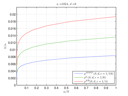
Refer to caption
Figure 11: Phase transition curves ρalg(δ;d,ϵ)superscript𝜌𝑎𝑙𝑔𝛿𝑑italic-ϵ\rho^{alg}\left(\delta;d,\epsilon\right) computed over finite values of δ(0,1)𝛿01\delta\in(0,1) with d𝑑d fixed and the different ϵitalic-ϵ\epsilon values for each algorithm - 1/4, 1/6 and 1/16 for ER, 1subscript1\ell_{1} and SSMP respectively.

Fig. 11 compares the phase transition plot of ρSSMP(δ;d,ϵ)superscript𝜌𝑆𝑆𝑀𝑃𝛿𝑑italic-ϵ\rho^{SSMP}(\delta;d,\epsilon) for SSMP (also for EMP and SMP), the phase transition of plot ρER(δ;d,ϵ)superscript𝜌𝐸𝑅𝛿𝑑italic-ϵ\rho^{ER}(\delta;d,\epsilon) for ER (also of LDDSR) and the phase transition plot of ρ1(δ;d,ϵ)superscript𝜌subscript1𝛿𝑑italic-ϵ\rho^{\ell_{1}}(\delta;d,\epsilon) for 1subscript1\ell_{1}-minimization. Remarkably, for ER and LDDSR recovery is guaranteed for a larger portion of the (δ,ρ)𝛿𝜌(\delta,\rho) plane than is guaranteed by the theory for 1subscript1\ell_{1}-minimization using sparse matrices; however, 1subscript1\ell_{1}-minimization has a larger recovery region than does SSMP, EMP, and SMP.
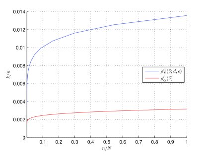
Refer to caption
Figure 12: Phase transition plots of 1subscript1\ell_{1}, ρG1(δ)subscriptsuperscript𝜌subscript1𝐺𝛿\rho^{\ell_{1}}_{G}\left(\delta\right), for Gaussian matrices derived using RIC2subscriptRIC2\mathrm{RIC}_{2} and ρE1(δ;d,ϵ)subscriptsuperscript𝜌subscript1𝐸𝛿𝑑italic-ϵ\rho^{\ell_{1}}_{E}\left(\delta;d,\epsilon\right) for adjacency matrices of expander graphs with n=1024𝑛1024n=1024, d=8𝑑8d=8, and ϵ=1/6italic-ϵ16\epsilon=1/6.

Fig. 12 shows a comparison of the phase transition of 1subscript1\ell_{1}-minimization as presented by Blanchard et. al. in [13] for dense Gaussian matrices based on RIC2subscriptRIC2\mathrm{RIC}_{2} analysis and the phase transition we derived here for the sparse binary matrices coming from lossless expander based on RIC1subscriptRIC1\mathrm{RIC}_{1} analysis. This shows a remarkable difference between the two with sparse matrices having better performance guarantees. However, these improved recovery guarantees are likely more due to the closer match of the method of analysis than to the efficacy of sparse matrices over dense matrices.

IV Proof of mains results

IV-A Proof of Theorem I.6

By the dyadic splitting |As|=|As21As22|subscript𝐴𝑠superscriptsubscript𝐴𝑠21superscriptsubscript𝐴𝑠22\left|A_{s}\right|=\left|A_{\lceil\frac{s}{2}\rceil}^{1}\cup A_{\lfloor\frac{s}{2}\rfloor}^{2}\right| and therefore

Prob(|As|as)=Prob(|As21As22|as)Probsubscript𝐴𝑠subscript𝑎𝑠Probsuperscriptsubscript𝐴𝑠21superscriptsubscript𝐴𝑠22subscript𝑎𝑠\displaystyle\hbox{Prob}\left(\left|A_{s}\right|\leq a_{s}\right)=\hbox{Prob}\left(\left|A_{\lceil\frac{s}{2}\rceil}^{1}\cup A_{\lfloor\frac{s}{2}\rfloor}^{2}\right|\leq a_{s}\right) (70)
=lsls2,ls2Prob(|As21As22|=ls)absentsubscriptsubscript𝑙𝑠subscriptsubscript𝑙𝑠2subscript𝑙𝑠2Probsuperscriptsubscript𝐴𝑠21superscriptsubscript𝐴𝑠22subscript𝑙𝑠\displaystyle=\sum_{l_{s}}\sum_{l_{\lceil\frac{s}{2}\rceil},l_{\lfloor\frac{s}{2}\rfloor}}\hbox{Prob}\left(\left|A_{\lceil\frac{s}{2}\rceil}^{1}\cup A_{\lfloor\frac{s}{2}\rfloor}^{2}\right|=l_{s}\right) (71)
=lsls21ls22Pn(ls,ls21,ls22)×\displaystyle=\sum_{l_{s}}\sum_{l_{\lceil\frac{s}{2}\rceil}^{1}}\sum_{l_{\lfloor\frac{s}{2}\rfloor}^{2}}\hbox{P}_{n}\left(l_{s},l_{\lceil\frac{s}{2}\rceil}^{1},l_{\lfloor\frac{s}{2}\rfloor}^{2}\right)\times
Prob(|As21|=ls21)Prob(|As22|=ls22).Probsuperscriptsubscript𝐴𝑠21superscriptsubscript𝑙𝑠21Probsuperscriptsubscript𝐴𝑠22superscriptsubscript𝑙𝑠22\displaystyle\qquad\hbox{Prob}\left(\left|A_{\lceil\frac{s}{2}\rceil}^{1}\right|=l_{\lceil\frac{s}{2}\rceil}^{1}\right)\hbox{Prob}\left(\left|A_{\lfloor\frac{s}{2}\rfloor}^{2}\right|=l_{\lfloor\frac{s}{2}\rfloor}^{2}\right). (72)

From (70) to (71) we sum over all possible events while from (71) to (IV-A), in line with the splitting technique, we simplify the probability to the product of the probabilities of the cardinalities of |As21|superscriptsubscript𝐴𝑠21\left|A_{\lceil\frac{s}{2}\rceil}^{1}\right| and |As22|superscriptsubscript𝐴𝑠22\left|A_{\lfloor\frac{s}{2}\rfloor}^{2}\right| and their intersection.

In a slight abuse of notation we write ljj=1,,xsubscriptsubscriptsuperscript𝑙𝑗𝑗1𝑥\mathop{\sum_{l^{j}}}_{j=1,\ldots,x} to denote applying the sum x𝑥x times. Now we use Lemma II.5 to simplify (IV-A) as follows.

lQ0j1j1=1,,q0lQ1j2j2=1,,q1lR1j3j3=1,,r1Pn(lQ0j1,lQ022j11,lQ022j1)×j2=1q1Prob(|AQ1j2|=lQ1j2)×j3=q1+1q1+r1Prob(|AR1j3|=lR1j3).subscriptsubscriptsubscriptsuperscript𝑙subscript𝑗1subscript𝑄0subscript𝑗11subscript𝑞0subscriptsubscriptsubscriptsuperscript𝑙subscript𝑗2subscript𝑄1subscript𝑗21subscript𝑞1subscriptsubscriptsubscriptsuperscript𝑙subscript𝑗3subscript𝑅1subscript𝑗31subscript𝑟1subscriptP𝑛subscriptsuperscript𝑙subscript𝑗1subscript𝑄0subscriptsuperscript𝑙2subscript𝑗11subscript𝑄02subscriptsuperscript𝑙2subscript𝑗1subscript𝑄02superscriptsubscriptproductsubscript𝑗21subscript𝑞1Probsubscriptsuperscript𝐴subscript𝑗2subscript𝑄1subscriptsuperscript𝑙subscript𝑗2subscript𝑄1superscriptsubscriptproductsubscript𝑗3subscript𝑞11subscript𝑞1subscript𝑟1Probsubscriptsuperscript𝐴subscript𝑗3subscript𝑅1subscriptsuperscript𝑙subscript𝑗3subscript𝑅1\mathop{\sum_{l^{j_{1}}_{Q_{0}}}}_{j_{1}=1,\ldots,q_{0}}\mathop{\sum_{l^{j_{2}}_{Q_{1}}}}_{j_{2}=1,\ldots,q_{1}}\mathop{\sum_{l^{j_{3}}_{R_{1}}}}_{j_{3}=1,\ldots,r_{1}}\hbox{P}_{n}\left(l^{j_{1}}_{Q_{0}},l^{2j_{1}-1}_{\lceil\frac{Q_{0}}{2}\rceil},l^{2j_{1}}_{\lfloor\frac{Q_{0}}{2}\rfloor}\right)\\ \times\prod_{j_{2}=1}^{q_{1}}\hbox{Prob}\left(\left|A^{j_{2}}_{Q_{1}}\right|=l^{j_{2}}_{Q_{1}}\right)\\ \times\prod_{j_{3}=q_{1}+1}^{q_{1}+r_{1}}\hbox{Prob}\left(\left|A^{j_{3}}_{R_{1}}\right|=l^{j_{3}}_{R_{1}}\right). (73)

Let’s quickly verify that (73) is the same as (IV-A). By Lemma II.5, Q0=ssubscript𝑄0𝑠Q_{0}=s is the number of columns in the set at the zeroth level of the split while q0=1subscript𝑞01q_{0}=1 is the number of sets with Q0subscript𝑄0Q_{0} columns at the zeroth level of the split. Thus for j1=1subscript𝑗11j_{1}=1 the first summation and the Pn()subscriptP𝑛\hbox{P}_{n}(\cdot) term are the same in the two equations. If Q02=Q02subscript𝑄02subscript𝑄02\lceil\frac{Q_{0}}{2}\rceil=\lfloor\frac{Q_{0}}{2}\rfloor, then they are both equal to Q1subscript𝑄1Q_{1} and q1=2subscript𝑞12q_{1}=2 while r1=0subscript𝑟10r_{1}=0. If on the other hand Q02=Q02+1subscript𝑄02subscript𝑄021\lceil\frac{Q_{0}}{2}\rceil=\lfloor\frac{Q_{0}}{2}\rfloor+1, then q1=1subscript𝑞11q_{1}=1 and r1=1subscript𝑟11r_{1}=1. In either case we have the remaining part of the expression of (IV-A) i.e. the second two summations and the product of the two Prob()Prob\hbox{Prob}(\cdot).

Now we proceed with the splitting - note (73) stopped only at the first level. At the next level, the second, we will have q2subscript𝑞2q_{2} sets with Q2subscript𝑄2Q_{2} columns and r2subscript𝑟2r_{2} sets with R2subscript𝑅2R_{2} columns which leads to the following expression.

lQ0j1j1=1,,q0lQ1j2j2=1,,q1lR1j3j3=1,,r1Pn(lQ0j1,lQ022j11,lQ022j1)×[lQ2j4j4=1,,q2lR2j5j5=1,,r2Pn(lQ1j2,lQ122j21,lQ122j2)Pn(lR1j3,lR122j31,lR122j3)×j4=1q2Prob(|AQ1j4|=lQ1j4)j5=q2+1q2+r2Prob(|AR1j5|=lR1j5)].subscriptsubscriptsubscriptsuperscript𝑙subscript𝑗1subscript𝑄0subscript𝑗11subscript𝑞0subscriptsubscriptsubscriptsuperscript𝑙subscript𝑗2subscript𝑄1subscript𝑗21subscript𝑞1subscriptsubscriptsubscriptsuperscript𝑙subscript𝑗3subscript𝑅1subscript𝑗31subscript𝑟1subscriptP𝑛subscriptsuperscript𝑙subscript𝑗1subscript𝑄0subscriptsuperscript𝑙2subscript𝑗11subscript𝑄02subscriptsuperscript𝑙2subscript𝑗1subscript𝑄02delimited-[]subscriptsubscriptsubscriptsuperscript𝑙subscript𝑗4subscript𝑄2subscript𝑗41subscript𝑞2subscriptsubscriptsubscriptsuperscript𝑙subscript𝑗5subscript𝑅2subscript𝑗51subscript𝑟2subscriptP𝑛subscriptsuperscript𝑙subscript𝑗2subscript𝑄1subscriptsuperscript𝑙2subscript𝑗21subscript𝑄12subscriptsuperscript𝑙2subscript𝑗2subscript𝑄12subscriptP𝑛subscriptsuperscript𝑙subscript𝑗3subscript𝑅1subscriptsuperscript𝑙2subscript𝑗31subscript𝑅12subscriptsuperscript𝑙2subscript𝑗3subscript𝑅12superscriptsubscriptproductsubscript𝑗41subscript𝑞2Probsubscriptsuperscript𝐴subscript𝑗4subscript𝑄1subscriptsuperscript𝑙subscript𝑗4subscript𝑄1superscriptsubscriptproductsubscript𝑗5subscript𝑞21subscript𝑞2subscript𝑟2Probsubscriptsuperscript𝐴subscript𝑗5subscript𝑅1subscriptsuperscript𝑙subscript𝑗5subscript𝑅1\mathop{\sum_{l^{j_{1}}_{Q_{0}}}}_{j_{1}=1,\ldots,q_{0}}\mathop{\sum_{l^{j_{2}}_{Q_{1}}}}_{j_{2}=1,\ldots,q_{1}}\mathop{\sum_{l^{j_{3}}_{R_{1}}}}_{j_{3}=1,\ldots,r_{1}}\hbox{P}_{n}\left(l^{j_{1}}_{Q_{0}},l^{2j_{1}-1}_{\lceil\frac{Q_{0}}{2}\rceil},l^{2j_{1}}_{\lfloor\frac{Q_{0}}{2}\rfloor}\right)\\ \times\Bigg{[}\mathop{\sum_{l^{j_{4}}_{Q_{2}}}}_{j_{4}=1,\ldots,q_{2}}\mathop{\sum_{l^{j_{5}}_{R_{2}}}}_{j_{5}=1,\ldots,r_{2}}\hbox{P}_{n}\left(l^{j_{2}}_{Q_{1}},l^{2j_{2}-1}_{\lceil\frac{Q_{1}}{2}\rceil},l^{2j_{2}}_{\lfloor\frac{Q_{1}}{2}\rfloor}\right)\\ \hbox{P}_{n}\left(l^{j_{3}}_{R_{1}},l^{2j_{3}-1}_{\lceil\frac{R_{1}}{2}\rceil},l^{2j_{3}}_{\lfloor\frac{R_{1}}{2}\rfloor}\right)\times\prod_{j_{4}=1}^{q_{2}}\hbox{Prob}\left(\left|A^{j_{4}}_{Q_{1}}\right|=l^{j_{4}}_{Q_{1}}\right)\\ \prod_{j_{5}=q_{2}+1}^{q_{2}+r_{2}}\hbox{Prob}\left(\left|A^{j_{5}}_{R_{1}}\right|=l^{j_{5}}_{R_{1}}\right)\Bigg{]}. (74)

We continue this splitting of each instance of Prob()Prob\hbox{Prob}(\cdot) for log2s+1subscript2𝑠1\lceil\log_{2}s\rceil+1 levels (from level 00 to level log2ssubscript2𝑠\lceil\log_{2}s\rceil) until reaching sets with single columns. Note that for the resulting binary tree from the splitting it suffice to stop at level log2s1subscript2𝑠1\lceil\log_{2}s\rceil-1 as can be seen in Fig. 10, since at this level we have all the information required for the enumeration of the sets. By construction, at level log2ssubscript2𝑠\lceil\log_{2}s\rceil, omitted from Fig. 10, the probability that the single column has d𝑑d nonzeros is one. This process gives a complicated product of nested sums of Pn()subscriptP𝑛\hbox{P}_{n}(\cdot) which we express as

lQ0j1j1=1,,q0lQ1j2j2=1,,q1lR1j3j3=1,,r1Pn(lQ0j1,lQ022j11,lQ022j1)×[lQ2j4j4=1,,q2lR2j5j5=1,,r2Pn(lQ1j2,lQ122j21,lQ122j2)×Pn(lR1j3,lR122j31,lR122j3)[[lQlog2s1j2log2s2j2log2s2=1,,qjlog2s1Pn(l4j2log2s4,l22j2log2s41,l22j2log2s4)×Pn(l3j2log2s3,l22j2log2s31,d)×Pn(l2j2log2s2,d,d)]].\mathop{\sum_{l^{j_{1}}_{Q_{0}}}}_{j_{1}=1,\ldots,q_{0}}\mathop{\sum_{l^{j_{2}}_{Q_{1}}}}_{j_{2}=1,\ldots,q_{1}}\mathop{\sum_{l^{j_{3}}_{R_{1}}}}_{j_{3}=1,\ldots,r_{1}}\hbox{P}_{n}\left(l^{j_{1}}_{Q_{0}},l^{2j_{1}-1}_{\lceil\frac{Q_{0}}{2}\rceil},l^{2j_{1}}_{\lfloor\frac{Q_{0}}{2}\rfloor}\right)\\ \times\Bigg{[}\mathop{\sum_{l^{j_{4}}_{Q_{2}}}}_{j_{4}=1,\ldots,q_{2}}\mathop{\sum_{l^{j_{5}}_{R_{2}}}}_{j_{5}=1,\ldots,r_{2}}\hbox{P}_{n}\left(l^{j_{2}}_{Q_{1}},l^{2j_{2}-1}_{\lceil\frac{Q_{1}}{2}\rceil},l^{2j_{2}}_{\lfloor\frac{Q_{1}}{2}\rfloor}\right)\\ \times\hbox{P}_{n}\left(l^{j_{3}}_{R_{1}},l^{2j_{3}-1}_{\lceil\frac{R_{1}}{2}\rceil},l^{2j_{3}}_{\lfloor\frac{R_{1}}{2}\rfloor}\right)\cdot\Bigg{[}\ldots\Bigg{[}\mathop{\sum_{l^{j_{2\lceil\log_{2}s\rceil-2}}_{Q_{\lceil\log_{2}s\rceil-1}}}}_{j_{2\lceil\log_{2}s\rceil-2}=1,\ldots,q_{j_{\lceil\log_{2}s\rceil-1}}}\\ \hbox{P}_{n}\left(l^{j_{2\lceil\log_{2}s\rceil-4}}_{4},l^{2j_{2\lceil\log_{2}s\rceil-4}-1}_{2},l^{2j_{2\lceil\log_{2}s\rceil-4}}_{2}\right)\\ \times\hbox{P}_{n}\left(l^{j_{2\lceil\log_{2}s\rceil-3}}_{3},l^{2j_{2\lceil\log_{2}s\rceil-3}-1}_{2},d\right)\\ \times\hbox{P}_{n}\left(l^{j_{2\lceil\log_{2}s\rceil-2}}_{2},d,d\right)\Bigg{]}\ldots\Bigg{]}. (75)

Using the definition of Pn()subscriptP𝑛\hbox{P}_{n}(\cdot) in Lemma II.3 we bound (75) by bounding each Pn()subscriptP𝑛\hbox{P}_{n}(\cdot) as in (59) with a product of a polynomial, π()𝜋\pi(\cdot), and an exponential with exponent ψn()subscript𝜓𝑛\psi_{n}(\cdot).

lQ0j1j1=1,,q0lQ1j2j2=1,,q1lR1j3j3=1,,r1π(lQ0j1,lQ022j11,lQ022j1)×eψn(lQ0j1,lQ022j11,lQ022j1)[lQ2j4j4=1,,q2lR2j5j5=1,,r2π(lQ1j2,lQ122j21,lQ122j2)eψn(lQ1j2,lQ122j21,lQ122j2)×π(lR1j3,lR122j31,lR122j3)eψn(lR1j3,lR122j31,lR122j3)×[×[lQlog2s1j2log2s2j2log2s2=1,,qjlog2s1π(l4j2log2s4,l22j2log2s41,l22j2log2s4)×eψn(l4j2log2s4,l22j2log2s41,l22j2log2s4)×π(l3j2log2s3,l22j2log2s31,d)×eψn(l3j2log2s3,l22j2log2s31,d)×π(l2j2log2s2,d,d)eψn(l2j2log2s2,d,d)]].\mathop{\sum_{l^{j_{1}}_{Q_{0}}}}_{j_{1}=1,\ldots,q_{0}}\mathop{\sum_{l^{j_{2}}_{Q_{1}}}}_{j_{2}=1,\ldots,q_{1}}\mathop{\sum_{l^{j_{3}}_{R_{1}}}}_{j_{3}=1,\ldots,r_{1}}\pi\left(l^{j_{1}}_{Q_{0}},l^{2j_{1}-1}_{\lceil\frac{Q_{0}}{2}\rceil},l^{2j_{1}}_{\lfloor\frac{Q_{0}}{2}\rfloor}\right)\times\\ e^{\psi_{n}\left(l^{j_{1}}_{Q_{0}},l^{2j_{1}-1}_{\lceil\frac{Q_{0}}{2}\rceil},l^{2j_{1}}_{\lfloor\frac{Q_{0}}{2}\rfloor}\right)}\cdot\Bigg{[}\mathop{\sum_{l^{j_{4}}_{Q_{2}}}}_{j_{4}=1,\ldots,q_{2}}\mathop{\sum_{l^{j_{5}}_{R_{2}}}}_{j_{5}=1,\ldots,r_{2}}\\ \pi\left(l^{j_{2}}_{Q_{1}},l^{2j_{2}-1}_{\lceil\frac{Q_{1}}{2}\rceil},l^{2j_{2}}_{\lfloor\frac{Q_{1}}{2}\rfloor}\right)\cdot e^{\psi_{n}\left(l^{j_{2}}_{Q_{1}},l^{2j_{2}-1}_{\lceil\frac{Q_{1}}{2}\rceil},l^{2j_{2}}_{\lfloor\frac{Q_{1}}{2}\rfloor}\right)}\times\\ \pi\left(l^{j_{3}}_{R_{1}},l^{2j_{3}-1}_{\lceil\frac{R_{1}}{2}\rceil},l^{2j_{3}}_{\lfloor\frac{R_{1}}{2}\rfloor}\right)\cdot e^{\psi_{n}\left(l^{j_{3}}_{R_{1}},l^{2j_{3}-1}_{\lceil\frac{R_{1}}{2}\rceil},l^{2j_{3}}_{\lfloor\frac{R_{1}}{2}\rfloor}\right)}\\ \times\Bigg{[}\ldots\times\Bigg{[}\mathop{\sum_{l^{j_{2\lceil\log_{2}s\rceil-2}}_{Q_{\lceil\log_{2}s\rceil-1}}}}_{j_{2\lceil\log_{2}s\rceil-2}=1,\ldots,q_{j_{\lceil\log_{2}s\rceil-1}}}\\ \pi\left(l^{j_{2\lceil\log_{2}s\rceil-4}}_{4},l^{2j_{2\lceil\log_{2}s\rceil-4}-1}_{2},l^{2j_{2\lceil\log_{2}s\rceil-4}}_{2}\right)\\ \times e^{\psi_{n}\left(l^{j_{2\lceil\log_{2}s\rceil-4}}_{4},l^{2j_{2\lceil\log_{2}s\rceil-4}-1}_{2},l^{2j_{2\lceil\log_{2}s\rceil-4}}_{2}\right)}\\ \times\pi\left(l^{j_{2\lceil\log_{2}s\rceil-3}}_{3},l^{2j_{2\lceil\log_{2}s\rceil-3}-1}_{2},d\right)\\ \times e^{\psi_{n}\left(l^{j_{2\lceil\log_{2}s\rceil-3}}_{3},l^{2j_{2\lceil\log_{2}s\rceil-3}-1}_{2},d\right)}\times\\ \pi\left(l^{j_{2\lceil\log_{2}s\rceil-2}}_{2},d,d\right)\cdot e^{\psi_{n}\left(l^{j_{2\lceil\log_{2}s\rceil-2}}_{2},d,d\right)}\bigg{]}\ldots\Bigg{]}. (76)

Using Lemma II.6 we maximize the ψn()subscript𝜓𝑛\psi_{n}(\cdot) and hence the exponentials. If we maximize each by choosing l()subscript𝑙l_{(\cdot)} to be a()subscript𝑎a_{(\cdot)}, then we can pull the exponentials out of the product. The exponential will then have the exponent Ψn(as,,a2,d)subscriptΨ𝑛subscript𝑎𝑠subscript𝑎2𝑑\Psi_{n}\left(a_{s},\ldots,a_{2},d\right). The factor involving the π()𝜋\pi(\cdot) will be called Π(ls,,l2,d)Πsubscript𝑙𝑠subscript𝑙2𝑑\Pi\left(l_{s},\ldots,l_{2},d\right) and we have the following upper bound for (76).

Π(ls,,l2,d)exp[Ψn(as,,a2,d)],Πsubscript𝑙𝑠subscript𝑙2𝑑subscriptΨ𝑛subscript𝑎𝑠subscript𝑎2𝑑\Pi\left(l_{s},\ldots,l_{2},d\right)\cdot\exp\left[\Psi_{n}\left(a_{s},\ldots,a_{2},d\right)\right], (77)

where the exponent Ψn(as,,a2,d)subscriptΨ𝑛subscript𝑎𝑠subscript𝑎2𝑑\Psi_{n}\left(a_{s},\ldots,a_{2},d\right) is given by

ψn(aQ0,aQ02,aQ02)++ψn(a2,d,d).subscript𝜓𝑛subscript𝑎subscript𝑄0subscript𝑎subscript𝑄02subscript𝑎subscript𝑄02subscript𝜓𝑛subscript𝑎2𝑑𝑑\psi_{n}\left(a_{Q_{0}},a_{\lceil\frac{Q_{0}}{2}\rceil},a_{\lfloor\frac{Q_{0}}{2}\rfloor}\right)+\ldots+\psi_{n}\left(a_{2},d,d\right). (78)

Now we attempt to bound the probability of interest in (70). This task reduces to bounding Π(ls,,l2,d)Πsubscript𝑙𝑠subscript𝑙2𝑑\Pi\left(l_{s},\ldots,l_{2},d\right) and Ψn(as,,a2,d)subscriptΨ𝑛subscript𝑎𝑠subscript𝑎2𝑑\Psi_{n}\left(a_{s},\ldots,a_{2},d\right) in (77) and we start with the former, i.e. bounding Π(ls,,l2,d)Πsubscript𝑙𝑠subscript𝑙2𝑑\Pi\left(l_{s},\ldots,l_{2},d\right). We bound each sum of π()𝜋\pi(\cdot) in Π(ls,,l2,d)Πsubscript𝑙𝑠subscript𝑙2𝑑\Pi\left(l_{s},\ldots,l_{2},d\right) of (77) by the maximum of summations multiplied by the number of terms in the sum. From (63) we see that π()𝜋\pi(\cdot) is maximized when all the three arguments are the same and using Corollary II.11 we take largest possible arguments that are equal in the range of the summation. In this way the following proposition provides the bound we end up.

Proposition IV.1

Let’s make each summation over the sets with the same number of columns to have the same range where the range we take are the maximum possible for each such set. Let’s also maximize π()𝜋\pi(\cdot) where all its three input variables are equal and are equal to the maximum of the third variable. Then we bound each sum by the largest term in the sum multiplied by the number of terms. This scheme combined with Lemma II.5 give the following upper bound on Π(ls,,l2,d)Πsubscript𝑙𝑠subscript𝑙2𝑑\Pi\left(l_{s},\ldots,l_{2},d\right).

(Q02d(54)22πQ02d)q0×j=1log2s2[(Qj2d(54)22πQj2d)qj×(Rj2d(54)22πRj2d)rj]×(Qlog2s12d(54)22πQlog2s12d)qlog2s1superscriptsubscript𝑄02𝑑superscript5422𝜋subscript𝑄02𝑑subscript𝑞0superscriptsubscriptproduct𝑗1subscript2𝑠2delimited-[]superscriptsubscript𝑄𝑗2𝑑superscript5422𝜋subscript𝑄𝑗2𝑑subscript𝑞𝑗superscriptsubscript𝑅𝑗2𝑑superscript5422𝜋subscript𝑅𝑗2𝑑subscript𝑟𝑗superscriptsubscript𝑄subscript2𝑠12𝑑superscript5422𝜋subscript𝑄subscript2𝑠12𝑑subscript𝑞subscript2𝑠1\left(\bigg{\lceil}\frac{Q_{0}}{2}\bigg{\rceil}d\left(\frac{5}{4}\right)^{2}\sqrt{2\pi\bigg{\lfloor}\frac{Q_{0}}{2}\bigg{\rfloor}d}\right)^{q_{0}}\times\\ \prod_{j=1}^{\lceil\log_{2}s\rceil-2}\left[\left(\bigg{\lceil}\frac{Q_{j}}{2}\bigg{\rceil}d\left(\frac{5}{4}\right)^{2}\sqrt{2\pi\bigg{\lfloor}\frac{Q_{j}}{2}\bigg{\rfloor}d}\right)^{q_{j}}\right.\times\\ \left.\left(\bigg{\lceil}\frac{R_{j}}{2}\bigg{\rceil}d\left(\frac{5}{4}\right)^{2}\sqrt{2\pi\bigg{\lfloor}\frac{R_{j}}{2}\bigg{\rfloor}d}\right)^{r_{j}}\right]\times\\ \left(\bigg{\lceil}\frac{Q_{\lceil\log_{2}s\rceil-1}}{2}\bigg{\rceil}d\left(\frac{5}{4}\right)^{2}\sqrt{2\pi\bigg{\lfloor}\frac{Q_{\lceil\log_{2}s\rceil-1}}{2}\bigg{\rfloor}d}\right)^{q_{\lceil\log_{2}s\rceil-1}} (79)
Proof:

From (63) we have

π(y,y,y)=(54)22πy(ny)n<(54)22πy.𝜋𝑦𝑦𝑦superscript5422𝜋𝑦𝑛𝑦𝑛superscript5422𝜋𝑦\pi(y,y,y)=\left(\frac{5}{4}\right)^{2}\sqrt{\frac{2\pi y(n-y)}{n}}<\left(\frac{5}{4}\right)^{2}\sqrt{2\pi y}. (80)

Simply put, we bound xπ(x,y,z)subscript𝑥𝜋𝑥𝑦𝑧\sum_{x}\pi(x,y,z) by multiplying the maximum of π(x,y,z)𝜋𝑥𝑦𝑧\pi(x,y,z) with the number of terms in the summation. Remember the order of magnitude of the arguments of π(x,y,z)𝜋𝑥𝑦𝑧\pi(x,y,z) is xyz𝑥𝑦𝑧x\geq y\geq z. Therefore, the maximum of π(x,y,z)𝜋𝑥𝑦𝑧\pi(x,y,z) occurs when the arguments are all equal to the maximum value of z𝑧z. In our splitting scheme the maximum possible value of lQj2subscript𝑙subscript𝑄𝑗2l_{\big{\lfloor}\frac{Q_{j}}{2}\big{\rfloor}} is Qj2dsubscript𝑄𝑗2𝑑\big{\lfloor}\frac{Q_{j}}{2}\big{\rfloor}\cdot d since there are d𝑑d nonzeros in each column. Also lQj2lQjlQj2+lQj2subscript𝑙subscript𝑄𝑗2subscript𝑙subscript𝑄𝑗subscript𝑙subscript𝑄𝑗2subscript𝑙subscript𝑄𝑗2l_{\big{\lfloor}\frac{Q_{j}}{2}\big{\rfloor}}\leq l_{Q_{j}}\leq l_{\big{\lfloor}\frac{Q_{j}}{2}\big{\rfloor}}+l_{\big{\lceil}\frac{Q_{j}}{2}\big{\rceil}} so the number of terms in the summation over lQjsubscript𝑙subscript𝑄𝑗l_{Q_{j}} is Qj2dsubscript𝑄𝑗2𝑑\big{\lceil}\frac{Q_{j}}{2}\big{\rceil}\cdot d, and similarly for Rjsubscript𝑅𝑗R_{j}. We know the values of the Qjsubscript𝑄𝑗Q_{j} and the Rjsubscript𝑅𝑗R_{j} and their quantities qjsubscript𝑞𝑗q_{j} and rjsubscript𝑟𝑗r_{j} respectively from Lemma II.5.

We replace y𝑦y by Qj2dsubscript𝑄𝑗2𝑑\big{\lfloor}\frac{Q_{j}}{2}\big{\rfloor}\cdot d or Rj2dsubscript𝑅𝑗2𝑑\big{\lfloor}\frac{R_{j}}{2}\big{\rfloor}\cdot d accordingly into the bound of π(y,y,y)𝜋𝑦𝑦𝑦\pi(y,y,y) in (80) and multiply by the number of terms in the summation, i.e. Qj2dsubscript𝑄𝑗2𝑑\big{\lceil}\frac{Q_{j}}{2}\big{\rceil}\cdot d or Rj2dsubscript𝑅𝑗2𝑑\big{\lceil}\frac{R_{j}}{2}\big{\rceil}\cdot d. This product is then repeated qjsubscript𝑞𝑗q_{j} or rjsubscript𝑟𝑗r_{j} times accordingly until the last level of the split, j=log2s1𝑗subscript2𝑠1j=\lceil\log_{2}s\rceil-1, where we have qlog2s1subscript𝑞subscript2𝑠1q_{\lceil\log_{2}s\rceil-1} and Qlog2s1subscript𝑄subscript2𝑠1Q_{\lceil\log_{2}s\rceil-1} (which is equal to 2). We exclude Rlog2s1subscript𝑅subscript2𝑠1R_{\lceil\log_{2}s\rceil-1} since lRlog2s1=dsubscript𝑙subscript𝑅subscript2𝑠1𝑑l_{R_{\lceil\log_{2}s\rceil-1}}=d. Putting the whole product together results to (79) hence concluding the proof of Proposition IV.1. ∎

As a final step we need the following corollary.

Corollary IV.2
Π(ls,,l2,d)<2252πs3d3exp[3slog(5d)].Πsubscript𝑙𝑠subscript𝑙2𝑑2252𝜋superscript𝑠3superscript𝑑33𝑠5𝑑\Pi\left(l_{s},\ldots,l_{2},d\right)<\frac{2}{25\sqrt{2\pi s^{3}d^{3}}}\cdot\exp\left[3s\log(5d)\right]. (81)
Proof:

From Lemma II.5 we can upper bound Rjsubscript𝑅𝑗R_{j} by Qjsubscript𝑄𝑗Q_{j} . Consequently (79) is upper bounded by the following.

(Q02d(54)22πQ02d)q0×j=1log2s2(Qj2d(54)22πQj2d)qj+rj×(Qlog2s12d(54)22πQlog2s12d)qlog2s1superscriptsubscript𝑄02𝑑superscript5422𝜋subscript𝑄02𝑑subscript𝑞0superscriptsubscriptproduct𝑗1subscript2𝑠2superscriptsubscript𝑄𝑗2𝑑superscript5422𝜋subscript𝑄𝑗2𝑑subscript𝑞𝑗subscript𝑟𝑗superscriptsubscript𝑄subscript2𝑠12𝑑superscript5422𝜋subscript𝑄subscript2𝑠12𝑑subscript𝑞subscript2𝑠1\left(\bigg{\lceil}\frac{Q_{0}}{2}\bigg{\rceil}d\left(\frac{5}{4}\right)^{2}\sqrt{2\pi\bigg{\lfloor}\frac{Q_{0}}{2}\bigg{\rfloor}d}\right)^{q_{0}}\times\\ \prod_{j=1}^{\lceil\log_{2}s\rceil-2}\left(\bigg{\lceil}\frac{Q_{j}}{2}\bigg{\rceil}d\left(\frac{5}{4}\right)^{2}\sqrt{2\pi\bigg{\lfloor}\frac{Q_{j}}{2}\bigg{\rfloor}d}\right)^{q_{j}+r_{j}}\times\\ \left(\bigg{\lceil}\frac{Q_{\lceil\log_{2}s\rceil-1}}{2}\bigg{\rceil}d\left(\frac{5}{4}\right)^{2}\sqrt{2\pi\bigg{\lfloor}\frac{Q_{\lceil\log_{2}s\rceil-1}}{2}\bigg{\rfloor}d}\right)^{q_{\lceil\log_{2}s\rceil-1}} (82)

Now we use the property that qj+rj=2jsubscript𝑞𝑗subscript𝑟𝑗superscript2𝑗q_{j}+r_{j}=2^{j} for j=1,,log2s1𝑗1subscript2𝑠1j=1,\ldots,\lceil\log_{2}s\rceil-1 from Lemma II.5 to bound (82) by the following.

j=0log2s1(Qj2d(54)22πQj2d)2j.superscriptsubscriptproduct𝑗0subscript2𝑠1superscriptsubscript𝑄𝑗2𝑑superscript5422𝜋subscript𝑄𝑗2𝑑superscript2𝑗\prod_{j=0}^{\lceil\log_{2}s\rceil-1}\left(\bigg{\lceil}\frac{Q_{j}}{2}\bigg{\rceil}d\left(\frac{5}{4}\right)^{2}\sqrt{2\pi\bigg{\lfloor}\frac{Q_{j}}{2}\bigg{\rfloor}d}\right)^{2^{j}}. (83)

We have a strict upper bound when rlog2s10subscript𝑟subscript2𝑠10r_{\lceil\log_{2}s\rceil-1}\neq 0, which occurs when s𝑠s is not a power of 222, because then by qj+rj=2jsubscript𝑞𝑗subscript𝑟𝑗superscript2𝑗q_{j}+r_{j}=2^{j} we have qlog2s1+rlog2s1=2log2s1subscript𝑞subscript2𝑠1subscript𝑟subscript2𝑠1superscript2subscript2𝑠1q_{\lceil\log_{2}s\rceil-1}+r_{\lceil\log_{2}s\rceil-1}=2^{\lceil\log_{2}s\rceil-1}. In fact (83) is an overestimate for a large s𝑠s which is not a power of 222.

Note Qj=s2jsubscript𝑄𝑗𝑠superscript2𝑗Q_{j}=\big{\lceil}\frac{s}{2^{j}}\big{\rceil} by Lemma II.5. Thus Qj2=s2j+1subscript𝑄𝑗2𝑠superscript2𝑗1\Big{\lceil}\frac{Q_{j}}{2}\Big{\rceil}=\big{\lceil}\frac{s}{2^{j+1}}\big{\rceil} and Qj2s2j+1subscript𝑄𝑗2𝑠superscript2𝑗1\Big{\lfloor}\frac{Q_{j}}{2}\Big{\rfloor}\leq\big{\lceil}\frac{s}{2^{j+1}}\big{\rceil}. So we bound (83) by the following.

j=0log2s1(s2j+1d(54)22πs2j+1d)2jsuperscriptsubscriptproduct𝑗0subscript2𝑠1superscript𝑠superscript2𝑗1𝑑superscript5422𝜋𝑠superscript2𝑗1𝑑superscript2𝑗\prod_{j=0}^{\lceil\log_{2}s\rceil-1}\left(\Big{\lceil}\frac{s}{2^{j+1}}\Big{\rceil}d\left(\frac{5}{4}\right)^{2}\sqrt{2\pi\Big{\lceil}\frac{s}{2^{j+1}}\Big{\rceil}d}\right)^{2^{j}} (84)

Next we upper bound log2s1subscript2𝑠1\lceil\log_{2}s\rceil-1 in the limit of the product by log2ssubscript2𝑠\log_{2}s and upper bound s2j+1𝑠superscript2𝑗1\lceil\frac{s}{2^{j+1}}\rceil by s2j+1+12=s2j+1(1+2j+1s)𝑠superscript2𝑗112𝑠superscript2𝑗11superscript2𝑗1𝑠\frac{s}{2^{j+1}}+\frac{1}{2}=\frac{s}{2^{j+1}}\left(1+\frac{2^{j+1}}{s}\right), we also move the d𝑑d into the square root and combined the constants to have the following bound on (84).

j=0log2s[s2j+1(1+2j+1s)(252π16)×s2j+1(1+2j+1s)d3]2j.superscriptsubscriptproduct𝑗0subscript2𝑠superscriptdelimited-[]𝑠superscript2𝑗11superscript2𝑗1𝑠252𝜋16𝑠superscript2𝑗11superscript2𝑗1𝑠superscript𝑑3superscript2𝑗\prod_{j=0}^{\log_{2}s}\left[\frac{s}{2^{j+1}}\left(1+\frac{2^{j+1}}{s}\right)\left(\frac{25\sqrt{2\pi}}{16}\right)\right.\times\\ \left.\sqrt{\frac{s}{2^{j+1}}\left(1+\frac{2^{j+1}}{s}\right)d^{3}}\right]^{2^{j}}. (85)

We bound (1+2j+1s)1superscript2𝑗1𝑠\left(1+\frac{2^{j+1}}{s}\right) by 222 to bound the above by

j=0log2s[s2j(252π16)s2jd3]2j=j=0log2s[(252π16)s3d323j]2jsuperscriptsubscriptproduct𝑗0subscript2𝑠superscriptdelimited-[]𝑠superscript2𝑗252𝜋16𝑠superscript2𝑗superscript𝑑3superscript2𝑗superscriptsubscriptproduct𝑗0subscript2𝑠superscriptdelimited-[]252𝜋16superscript𝑠3superscript𝑑3superscript23𝑗superscript2𝑗\prod_{j=0}^{\log_{2}s}\left[\frac{s}{2^{j}}\left(\frac{25\sqrt{2\pi}}{16}\right)\sqrt{\frac{s}{2^{j}}d^{3}}\right]^{2^{j}}\\ =\prod_{j=0}^{\log_{2}s}\left[\left(\frac{25\sqrt{2\pi}}{16}\right)\sqrt{\frac{s^{3}d^{3}}{2^{3j}}}\right]^{2^{j}} (86)

where we moved s/2j𝑠superscript2𝑗s/2^{j} into the square root. Using the rule of indices the product of the constant term is replaced by it’s power to sum of the indices. We then rearranged to have the power 3/2323/2 in the outside and this gives the following.

(252π16)i=0log2s2i[j=0log2s(sd2j)2j]3/2superscript252𝜋16superscriptsubscript𝑖0subscript2𝑠superscript2𝑖superscriptdelimited-[]superscriptsubscriptproduct𝑗0subscript2𝑠superscript𝑠𝑑superscript2𝑗superscript2𝑗32\displaystyle\left(\frac{25\sqrt{2\pi}}{16}\right)^{\sum_{i=0}^{\log_{2}s}2^{i}}\left[\prod_{j=0}^{\log_{2}s}\left(\frac{sd}{2^{j}}\right)^{2^{j}}\right]^{3/2} (87)
=(252π16)2s1[(sd)i=0log2s2ij=0log2s(12j)2j]3/2absentsuperscript252𝜋162𝑠1superscriptdelimited-[]superscript𝑠𝑑superscriptsubscript𝑖0subscript2𝑠superscript2𝑖superscriptsubscriptproduct𝑗0subscript2𝑠superscript1superscript2𝑗superscript2𝑗32\displaystyle=\left(\frac{25\sqrt{2\pi}}{16}\right)^{2s-1}\left[\left(sd\right)^{\sum_{i=0}^{\log_{2}s}2^{i}}\prod_{j=0}^{\log_{2}s}\left(\frac{1}{2^{j}}\right)^{2^{j}}\right]^{3/2} (88)
=(252π16)2s1[(sd)2s1(12)j=0log2sj2j]3/2.absentsuperscript252𝜋162𝑠1superscriptdelimited-[]superscript𝑠𝑑2𝑠1superscript12superscriptsubscript𝑗0subscript2𝑠𝑗superscript2𝑗32\displaystyle=\left(\frac{25\sqrt{2\pi}}{16}\right)^{2s-1}\left[\left(sd\right)^{2s-1}\left(\frac{1}{2}\right)^{\sum_{j=0}^{\log_{2}s}j2^{j}}\right]^{3/2}. (89)

From (87) to (88) we evaluate the power of the first factor which is a geometric series and we again use the rule of indices for the sd𝑠𝑑sd factor. Then from (88) to (89) we use the indices’ rule for the last factor and evaluate the power of the sd𝑠𝑑sd factor which is also a geometric series. We simplify the power of the last factor by using the following.

k=1mk2k=(m1)2m+1+2.superscriptsubscript𝑘1𝑚𝑘superscript2𝑘𝑚1superscript2𝑚12\sum_{k=1}^{m}k\cdot 2^{k}=(m-1)\cdot 2^{m+1}+2. (90)

This therefore simplifies (89) as follows.

(252π16)2s1[(sd)2s1(12)(log2s1)2log2s+1+2]3/2superscript252𝜋162𝑠1superscriptdelimited-[]superscript𝑠𝑑2𝑠1superscript12subscript2𝑠1superscript2subscript2𝑠1232\displaystyle\left(\frac{25\sqrt{2\pi}}{16}\right)^{2s-1}\left[\left(sd\right)^{2s-1}\left(\frac{1}{2}\right)^{(\log_{2}s-1)\cdot 2^{\log_{2}s+1}+2}\right]^{3/2} (91)
=(252π16)2s1[(sd)2s1(12)2s(log2s1)14]3/2absentsuperscript252𝜋162𝑠1superscriptdelimited-[]superscript𝑠𝑑2𝑠1superscript122𝑠subscript2𝑠11432\displaystyle=\left(\frac{25\sqrt{2\pi}}{16}\right)^{2s-1}\left[\left(sd\right)^{2s-1}\left(\frac{1}{2}\right)^{2s(\log_{2}s-1)}\frac{1}{4}\right]^{3/2} (92)
=(252π16)2s1[(sd)2s4sd22slog2s22s]3/2absentsuperscript252𝜋162𝑠1superscriptdelimited-[]superscript𝑠𝑑2𝑠4𝑠𝑑superscript22𝑠subscript2𝑠superscript22𝑠32\displaystyle=\left(\frac{25\sqrt{2\pi}}{16}\right)^{2s-1}\left[\frac{(sd)^{2s}}{4sd}2^{-2s\log_{2}s}2^{2s}\right]^{3/2} (93)
=(252π16)2s(16252π)[(2sd)2s4sds2s]3/2absentsuperscript252𝜋162𝑠16252𝜋superscriptdelimited-[]superscript2𝑠𝑑2𝑠4𝑠𝑑superscript𝑠2𝑠32\displaystyle=\left(\frac{25\sqrt{2\pi}}{16}\right)^{2s}\left(\frac{16}{25\sqrt{2\pi}}\right)\left[\frac{(2sd)^{2s}}{4sd}s^{-2s}\right]^{3/2} (94)
=(252π16)2s(16252π)[(2d)2s4sd]3/2.absentsuperscript252𝜋162𝑠16252𝜋superscriptdelimited-[]superscript2𝑑2𝑠4𝑠𝑑32\displaystyle=\left(\frac{25\sqrt{2\pi}}{16}\right)^{2s}\left(\frac{16}{25\sqrt{2\pi}}\right)\left[\frac{(2d)^{2s}}{4sd}\right]^{3/2}. (95)

From (91) through (93) we simplified using basic properties of indices and logarithms. While from (93) to (94) we incorporated 22ssuperscript22𝑠2^{2s} into the first factor inside the square brackets and we rewrote the first factor into a product of a power in s𝑠s and another without s𝑠s. From (94) to (95) the s2ssuperscript𝑠2𝑠s^{2s} and s2ssuperscript𝑠2𝑠s^{-2s} canceled out.

Now we expand the square brackets in (95) to have (96) below.

(252π16)2s(16252π)18s3d3(2d)3ssuperscript252𝜋162𝑠16252𝜋18superscript𝑠3superscript𝑑3superscript2𝑑3𝑠\displaystyle\left(\frac{25\sqrt{2\pi}}{16}\right)^{2s}\left(\frac{16}{25\sqrt{2\pi}}\right)\frac{1}{8\sqrt{s^{3}d^{3}}}(2d)^{3s} (96)
=(252π16)2s(2d)3s2252πs3d3absentsuperscript252𝜋162𝑠superscript2𝑑3𝑠2252𝜋superscript𝑠3superscript𝑑3\displaystyle=\left(\frac{25\sqrt{2\pi}}{16}\right)^{2s}(2d)^{3s}\frac{2}{25\sqrt{2\pi s^{3}d^{3}}} (97)
=2252πs3d3exp(3slog(2(252π16)2/3d))absent2252𝜋superscript𝑠3superscript𝑑33𝑠2superscript252𝜋1623𝑑\displaystyle=\frac{2}{25\sqrt{2\pi s^{3}d^{3}}}\cdot\exp\left(3s\log\left(2\left(\frac{25\sqrt{2\pi}}{16}\right)^{2/3}d\right)\right) (98)
<2252πs3d3exp[3slog(5d)]absent2252𝜋superscript𝑠3superscript𝑑33𝑠5𝑑\displaystyle<\frac{2}{25\sqrt{2\pi s^{3}d^{3}}}\cdot\exp\left[3s\log(5d)\right] (99)

From (96) to (97) we simplified and from (97) to (98) we rewrote the powers as an exponential with a logarithmic exponent. Then from (98) to (99) we upper bounded 2(252π16)2/32superscript252𝜋16232\left(\frac{25\sqrt{2\pi}}{16}\right)^{2/3} by 555 which gives the required format of a product of a polynomial and an exponential to conclude the proof. ∎

With the bound in Corollary IV.2 we have completed the bounding of Π(ls,,l2,d)Πsubscript𝑙𝑠subscript𝑙2𝑑\Pi\left(l_{s},\ldots,l_{2},d\right) in (77). Next we bound Ψn(as,,a2,d)subscriptΨ𝑛subscript𝑎𝑠subscript𝑎2𝑑\Psi_{n}\left(a_{s},\ldots,a_{2},d\right) which is given by (78). Lemma II.5 gives the three arguments for each ψn()subscript𝜓𝑛\psi_{n}(\cdot) and the number of ψn()subscript𝜓𝑛\psi_{n}(\cdot) with the same arguments. Using this lemma we express Ψn(as,,a2,d)subscriptΨ𝑛subscript𝑎𝑠subscript𝑎2𝑑\Psi_{n}\left(a_{s},\ldots,a_{2},d\right) as

j=0log2(s)2[qjψn(aQj,aQj2,aQj2)+rjψn(aRj,aRj2,aRj2)]+qlog2(s)1ψn(a2,d,d).superscriptsubscript𝑗0subscript2𝑠2delimited-[]subscript𝑞𝑗subscript𝜓𝑛subscript𝑎subscript𝑄𝑗subscript𝑎subscript𝑄𝑗2subscript𝑎subscript𝑄𝑗2subscript𝑟𝑗subscript𝜓𝑛subscript𝑎subscript𝑅𝑗subscript𝑎subscript𝑅𝑗2subscript𝑎subscript𝑅𝑗2subscript𝑞subscript2𝑠1subscript𝜓𝑛subscript𝑎2𝑑𝑑\sum_{j=0}^{\lceil\log_{2}(s)\rceil-2}\left[q_{j}\cdot\psi_{n}\left(a_{Q_{j}},a_{\big{\lceil}\frac{Q_{j}}{2}\big{\rceil}},a_{\big{\lfloor}\frac{Q_{j}}{2}\big{\rfloor}}\right)+\right.\\ \left.r_{j}\cdot\psi_{n}\left(a_{R_{j}},a_{\big{\lceil}\frac{R_{j}}{2}\big{\rceil}},a_{\big{\lfloor}\frac{R_{j}}{2}\big{\rfloor}}\right)\right]+\\ q_{\lceil\log_{2}(s)\rceil-1}\cdot\psi_{n}\left(a_{2},d,d\right). (100)

Equation (100) is bounded above in Lemma II.7 by the following.

j=0log2(s)12jψn(aQj,aRj2,aRj2).superscriptsubscript𝑗0subscript2𝑠1superscript2𝑗subscript𝜓𝑛subscript𝑎subscript𝑄𝑗subscript𝑎subscript𝑅𝑗2subscript𝑎subscript𝑅𝑗2\sum_{j=0}^{\lceil\log_{2}(s)\rceil-1}2^{j}\cdot\psi_{n}\left(a_{Q_{j}},a_{\big{\lfloor}\frac{R_{j}}{2}\big{\rfloor}},a_{\big{\lfloor}\frac{R_{j}}{2}\big{\rfloor}}\right). (101)

If we let the a2i=aQjsubscript𝑎2𝑖subscript𝑎subscript𝑄𝑗a_{2i}=a_{Q_{j}} and ai=aRj2subscript𝑎𝑖subscript𝑎subscript𝑅𝑗2a_{i}=a_{\big{\lfloor}\frac{R_{j}}{2}\big{\rfloor}} we have (101) equal to the following.

i=1s/2s2iψn(a2i,ai,ai)=i=1s/2s2i[aiH(a2iaiai)+(nai)H(a2iainai)nH(ain)].superscriptsubscript𝑖1𝑠2𝑠2𝑖subscript𝜓𝑛subscript𝑎2𝑖subscript𝑎𝑖subscript𝑎𝑖superscriptsubscript𝑖1𝑠2𝑠2𝑖delimited-[]subscript𝑎𝑖Hsubscript𝑎2𝑖subscript𝑎𝑖subscript𝑎𝑖𝑛subscript𝑎𝑖Hsubscript𝑎2𝑖subscript𝑎𝑖𝑛subscript𝑎𝑖𝑛Hsubscript𝑎𝑖𝑛\sum_{i=1}^{\lceil s/2\rceil}\frac{s}{2i}\cdot\psi_{n}\left(a_{2i},a_{i},a_{i}\right)=\sum_{i=1}^{\lceil s/2\rceil}\frac{s}{2i}\left[a_{i}\cdot\hbox{H}\left(\frac{a_{2i}-a_{i}}{a_{i}}\right)\right.\\ \left.+\left(n-a_{i}\right)\cdot\hbox{H}\left(\frac{a_{2i}-a_{i}}{n-a_{i}}\right)-n\cdot\hbox{H}\left(\frac{a_{i}}{n}\right)\right]. (102)

Now we combine the bound of Π(ls,,l2,d)Πsubscript𝑙𝑠subscript𝑙2𝑑\Pi\left(l_{s},\ldots,l_{2},d\right) in (81) and the exponential whose exponent is the bound of Ψn(as,,a2,d)subscriptΨ𝑛subscript𝑎𝑠subscript𝑎2𝑑\Psi_{n}\left(a_{s},\ldots,a_{2},d\right) in (102) to get (2), the polynomial pmax(s,d)=2252πs3d3subscript𝑝𝑚𝑎𝑥𝑠𝑑2252𝜋superscript𝑠3superscript𝑑3p_{max}(s,d)=\frac{2}{25\sqrt{2\pi s^{3}d^{3}}}, and (3), the exponent of the exponential Ψ(as,,d)Ψsubscript𝑎𝑠𝑑\Psi\left(a_{s},\ldots,d\right) given by the sum of 3slog(5d)3𝑠5𝑑3s\log\left(5d\right) and the right hand side of (102).

Lemma II.8 gives the aisubscript𝑎𝑖a_{i} that maximize (102) and the systems (II.8) and (II.8) they satisfy depending on the constraints on assubscript𝑎𝑠a_{s}. Solving completely the system (II.8) gives a^isubscript^𝑎𝑖\hat{a}_{i} in (52) and (4) which are the expected values of the aisubscript𝑎𝑖a_{i}. The system (5) is equivalent to (II.8) hence also proven in Lemma II.8. This therefore concludes the proof Theorem I.6.

IV-B Main Corollaries

In this section we present the proofs of the corollaries in Sections I-A and I-B. These include the proof of Corollary I.7 in Section IV-B1, the proof of Corollary I.10 in Section IV-B2 and the proof of Corollary I.11 given in Section IV-B3.

IV-B1 Corollary I.7

Satisfying RIP-1 means that for any slimit-from𝑠s-sparse vector x𝑥x, ASx1(12ϵ)dx1subscriptnormsubscript𝐴𝑆𝑥112italic-ϵ𝑑subscriptnorm𝑥1\|A_{S}x\|_{1}\geq(1-2\epsilon)d\|x\|_{1} which indicates that the cardinality of the set of neighbors satisfies |As|(1ϵ)dssubscript𝐴𝑠1italic-ϵ𝑑𝑠|A_{s}|\geq(1-\epsilon)ds. Therefore

Prob(ASx1(12ϵ)dx1)Prob(|As|(1ϵ)ds).Probsubscriptdelimited-∥∥subscript𝐴𝑆𝑥112italic-ϵ𝑑subscriptdelimited-∥∥𝑥1Probsubscript𝐴𝑠1italic-ϵ𝑑𝑠\hbox{Prob}\left(\|A_{S}x\|_{1}\leq(1-2\epsilon)d\|x\|_{1}\right)\\ \equiv\hbox{Prob}\left(|A_{s}|\leq(1-\epsilon)ds\right). (103)

This implies that as=(1ϵ)dssubscript𝑎𝑠1italic-ϵ𝑑𝑠a_{s}=(1-\epsilon)ds and since this is restricting assubscript𝑎𝑠a_{s} to be less than it’s expected value given by (4), the rest of the aisubscript𝑎𝑖a_{i} satisfy the polynomial system (5). If there exists a solution then the aisubscript𝑎𝑖a_{i} would be functions of s,d𝑠𝑑s,~{}d and ϵitalic-ϵ\epsilon which makes Ψ(as,,a2,d)=Ψ(s,d,ϵ)Ψsubscript𝑎𝑠subscript𝑎2𝑑Ψ𝑠𝑑italic-ϵ\Psi\left(a_{s},\ldots,a_{2},d\right)=\Psi\left(s,d,\epsilon\right).

IV-B2 Corollary I.10

Corollary I.7 states that by fixing S𝑆S and the other parameters, Prob(ASx1(12ϵ)dx1)<pmax(s,d)exp[nΨ(s,d,ϵ)]Probsubscriptnormsubscript𝐴𝑆𝑥112italic-ϵ𝑑subscriptnorm𝑥1subscript𝑝𝑚𝑎𝑥𝑠𝑑𝑛Ψ𝑠𝑑italic-ϵ\hbox{Prob}\left(\mathop{\|A_{S}x\|_{1}}\leq(1-2\epsilon)d\|x\|_{1}\right)<p_{max}(s,d)\cdot\exp\left[n\cdot\Psi\left(s,d,\epsilon\right)\right]. Corollary I.10 considers any S[N]𝑆delimited-[]𝑁S\subset[N] and since the matrices are adjacency matrices of lossless expanders we need to consider any S[N]𝑆delimited-[]𝑁S\subset[N] such that |S|k𝑆𝑘|S|\leq k. Therefore our target is Prob(Ax1(12ϵ)dx1)Probsubscriptnorm𝐴𝑥112italic-ϵ𝑑subscriptnorm𝑥1\hbox{Prob}\left(\mathop{\|Ax\|_{1}}\leq(1-2\epsilon)d\|x\|_{1}\right) which is bounded by a simple union bound over all (Ns)Sbinomial𝑁𝑠𝑆\binom{N}{s}~{}S sets and by treating each set S𝑆S, of cardinality less than k𝑘k, independent we sum over this probability to get the following bound.

s=2k(Ns)Prob(ASx1(12ϵ)dx1)superscriptsubscript𝑠2𝑘binomial𝑁𝑠Probsubscriptnormsubscript𝐴𝑆𝑥112italic-ϵ𝑑subscriptnorm𝑥1\displaystyle\sum_{s=2}^{k}\binom{N}{s}\cdot\hbox{Prob}\left(\mathop{\|A_{S}x\|_{1}}\leq(1-2\epsilon)d\|x\|_{1}\right) (104)
<s=2k(Ns)pmax(s,d)exp[nΨ(s,d,ϵ)]absentsuperscriptsubscript𝑠2𝑘binomial𝑁𝑠subscript𝑝𝑚𝑎𝑥𝑠𝑑𝑛Ψ𝑠𝑑italic-ϵ\displaystyle<\sum_{s=2}^{k}\binom{N}{s}\cdot p_{max}(s,d)\cdot\exp\left[n\cdot\Psi\left(s,d,\epsilon\right)\right] (105)
<s=2k(54)212πs(1sN)pmax(s,d)absentsuperscriptsubscript𝑠2𝑘superscript54212𝜋𝑠1𝑠𝑁subscript𝑝𝑚𝑎𝑥𝑠𝑑\displaystyle<\sum_{s=2}^{k}\left(\frac{5}{4}\right)^{2}\frac{1}{\sqrt{2\pi s\left(1-\frac{s}{N}\right)}}\cdot p_{max}(s,d)
×exp[NH(sN)+nΨ(s,d,ϵ)]absent𝑁H𝑠𝑁𝑛Ψ𝑠𝑑italic-ϵ\displaystyle\quad\times\exp\left[N\hbox{H}\left(\frac{s}{N}\right)+n\cdot\Psi\left(s,d,\epsilon\right)\right] (106)
<k(54)2pmax(k,d)2πk(1kN)absent𝑘superscript542subscript𝑝𝑚𝑎𝑥𝑘𝑑2𝜋𝑘1𝑘𝑁\displaystyle<k\left(\frac{5}{4}\right)^{2}\frac{p_{max}(k,d)}{\sqrt{2\pi k\left(1-\frac{k}{N}\right)}}
×exp[N(H(kN)+nNΨ(k,d,ϵ))].absent𝑁H𝑘𝑁𝑛𝑁Ψ𝑘𝑑italic-ϵ\displaystyle\quad\times\exp\left[N\left(\hbox{H}\left(\frac{k}{N}\right)+\frac{n}{N}\cdot\Psi\left(k,d,\epsilon\right)\right)\right]. (107)

From (104) to (105) we bound the probability in (104) using Corollary I.7. Then from (105) to (IV-B2) we bound (Ns)binomial𝑁𝑠\binom{N}{s} using Stirling’s formula (64) by a polynomial in N𝑁N multiplying pmax(s,d)subscript𝑝𝑚𝑎𝑥𝑠𝑑p_{max}(s,d) and an exponential incorporated into the exponent of the exponential term. From (IV-B2) to (IV-B2) we use that for N>2k𝑁2𝑘N>2k the entropy H(sN)H𝑠𝑁\hbox{H}\left(\frac{s}{N}\right) is largest when s=k𝑠𝑘s=k and we bound the summation by taking the maximum value of s𝑠s and multiplying by the number of terms plus one, giving k𝑘k, in the summation. This gives pmax(N,k,d)=k(54)2pmax(k,d)2πk(1kN)subscriptsuperscript𝑝𝑚𝑎𝑥𝑁𝑘𝑑𝑘superscript542subscript𝑝𝑚𝑎𝑥𝑘𝑑2𝜋𝑘1𝑘𝑁p^{\prime}_{max}(N,k,d)=k\left(\frac{5}{4}\right)^{2}\frac{p_{max}(k,d)}{\sqrt{2\pi k\left(1-\frac{k}{N}\right)}} which simplifies to 116πkd3(1kN)116𝜋𝑘superscript𝑑31𝑘𝑁\frac{1}{16\pi k\sqrt{d^{3}\left(1-\frac{k}{N}\right)}} and the factor Ψnet(k,n,N;d,ϵ)=H(kN)+nNΨ(k,d,ϵ)subscriptΨ𝑛𝑒𝑡𝑘𝑛𝑁𝑑italic-ϵH𝑘𝑁𝑛𝑁Ψ𝑘𝑑italic-ϵ\Psi_{net}\left(k,n,N;d,\epsilon\right)=\hbox{H}\left(\frac{k}{N}\right)+\frac{n}{N}\cdot\Psi\left(k,d,\epsilon\right) is what is multiplied to N𝑁N in the exponent as claimed.

IV-B3 Corollary I.11

Corollary I.10 has given us an upper bound on the probability Prob(Ax1(12ϵ)dx1)Probsubscriptnorm𝐴𝑥112italic-ϵ𝑑subscriptnorm𝑥1\hbox{Prob}\left(\|Ax\|_{1}\leq(1-2\epsilon)d\|x\|_{1}\right) in (9). In this bound the exponential dominates the polynomial. Consequently, in the limit as (k,n,N)𝑘𝑛𝑁(k,n,N)\rightarrow\infty while k/nρ(0,1)𝑘𝑛𝜌01k/n\rightarrow\rho\in(0,1) and n/Nδ(0,1)𝑛𝑁𝛿01n/N\rightarrow\delta\in(0,1) this bound has a sharp transition at the zero level curve of ΨnetsubscriptΨ𝑛𝑒𝑡\Psi_{net}. For Ψnet(k,n,N;d,ϵ)subscriptΨ𝑛𝑒𝑡𝑘𝑛𝑁𝑑italic-ϵ\Psi_{net}\left(k,n,N;d,\epsilon\right) strictly bounded above zero the overall bound grows exponentially in N𝑁N without limit, while for Ψnet(k,n,N;d,ϵ)subscriptΨ𝑛𝑒𝑡𝑘𝑛𝑁𝑑italic-ϵ\Psi_{net}\left(k,n,N;d,\epsilon\right) strictly bounded below zero the overall bound decays to zero exponentially quickly. We define ρexp(δ;d,ϵ)superscript𝜌𝑒𝑥𝑝𝛿𝑑italic-ϵ\rho^{exp}(\delta;d,\epsilon) to satisfy Ψnet(k,n,N;d,ϵ)=0subscriptΨ𝑛𝑒𝑡𝑘𝑛𝑁𝑑italic-ϵ0\Psi_{net}\left(k,n,N;d,\epsilon\right)=0 in (13), so that for any ρ𝜌\rho strictly less than ρexp(δ;d,ϵ)superscript𝜌𝑒𝑥𝑝𝛿𝑑italic-ϵ\rho^{exp}(\delta;d,\epsilon) the exponent will satisfy Ψnet(k,n,N;d,ϵ)<0subscriptΨ𝑛𝑒𝑡𝑘𝑛𝑁𝑑italic-ϵ0\Psi_{net}\left(k,n,N;d,\epsilon\right)<0 and hence the bound decay to zero.

More precisely, for k/nρ<(1γ)ρexp(δ;d,ϵ)𝑘𝑛𝜌1𝛾superscript𝜌𝑒𝑥𝑝𝛿𝑑italic-ϵk/n\rightarrow\rho<(1-\gamma)\rho^{exp}(\delta;d,\epsilon) with small γ>0𝛾0\gamma>0, in this regime of ρ<(1γ)ρexp(δ;d,ϵ)𝜌1𝛾superscript𝜌𝑒𝑥𝑝𝛿𝑑italic-ϵ\rho<(1-\gamma)\rho^{exp}(\delta;d,\epsilon) we have Prob(Ax1(12ϵ)dx1)0Probsubscriptnorm𝐴𝑥112italic-ϵ𝑑subscriptnorm𝑥10\hbox{Prob}\left(\|Ax\|_{1}\leq(1-2\epsilon)d\|x\|_{1}\right)\rightarrow 0. Therefore, Prob(Ax1(12ϵ)dx1)1Probsubscriptnorm𝐴𝑥112italic-ϵ𝑑subscriptnorm𝑥11\hbox{Prob}\left(\|Ax\|_{1}\geq(1-2\epsilon)d\|x\|_{1}\right)\rightarrow 1 as the problem size grows such that (k,n,N)𝑘𝑛𝑁(k,n,N)\rightarrow\infty, n/Nδ(0,1)𝑛𝑁𝛿01n/N\rightarrow\delta\in(0,1) and k/nρ𝑘𝑛𝜌k/n\rightarrow\rho.

V Appendix

V-A Proof of Corollary II.2

The first part of this proof uses ideas from the proof of Proposition II.1 which is the same as Theorem 16 in [26]. We consider a bipartite graph G=(U,V,E)𝐺𝑈𝑉𝐸G=(U,V,E) with |U|=N𝑈𝑁|U|=N left vertices, |V|=n𝑉𝑛|V|=n right vertices and left degree d𝑑d. For a fixed SU𝑆𝑈S\subset U where |S|=sk𝑆𝑠𝑘|S|=s\leq k, G𝐺G fails to be an expander on S𝑆S if |Γ(S)|<(1ϵ)dsΓ𝑆1italic-ϵ𝑑𝑠|\Gamma(S)|<(1-\epsilon)ds. This means that in a sequence of ds𝑑𝑠ds vertex indices at least ϵdsitalic-ϵ𝑑𝑠\epsilon ds of the these indices are in the collision set that is identical to some preceding value in the sequence.

Therefore, the probability that a neighbor chosen uniformly at random is to be in the collision set is at most ds/n𝑑𝑠𝑛ds/n and, treating each event independently, then the probability that a set of ϵdsitalic-ϵ𝑑𝑠\epsilon ds neighbors chosen at random are in the collision set is at most (ds/n)ϵdssuperscript𝑑𝑠𝑛italic-ϵ𝑑𝑠\left(ds/n\right)^{\epsilon ds}. There are (dsϵds)binomial𝑑𝑠italic-ϵ𝑑𝑠\binom{ds}{\epsilon ds} ways of choosing a set of ϵdsitalic-ϵ𝑑𝑠\epsilon ds points from a set of ds𝑑𝑠ds points and (Ns)binomial𝑁𝑠\binom{N}{s} ways of choosing each set S𝑆S from U𝑈U. This means therefore that the probability that G𝐺G fails to expand in at least one of the sets S𝑆S of fixed size s𝑠s can be bounded above by a union bound

Prob(Gfails to expand onS)(Ns)(dsϵds)(dsn)ϵds.Prob𝐺fails to expand on𝑆binomial𝑁𝑠binomial𝑑𝑠italic-ϵ𝑑𝑠superscript𝑑𝑠𝑛italic-ϵ𝑑𝑠\hbox{Prob}\left(G~{}\mbox{fails to expand on}~{}S\right)\\ \leq\binom{N}{s}\binom{ds}{\epsilon ds}\left(\frac{ds}{n}\right)^{\epsilon ds}. (108)

We define pssubscript𝑝𝑠p_{s} to be the right hand side of (108) and we use the right hand side of the Stirling’s inequality (64) to upper bound pssubscript𝑝𝑠p_{s} as thus

ps<54[2πϵdsds(1ϵdsds)ϵds]12exp[dsH(ϵdsds)]×54[2πsN(1sN)N]12×exp[NH(sN)]×(dsn)ϵdssubscript𝑝𝑠54superscriptdelimited-[]2𝜋italic-ϵ𝑑𝑠𝑑𝑠1italic-ϵ𝑑𝑠𝑑𝑠italic-ϵ𝑑𝑠12𝑑𝑠Hitalic-ϵ𝑑𝑠𝑑𝑠54superscriptdelimited-[]2𝜋𝑠𝑁1𝑠𝑁𝑁12𝑁H𝑠𝑁superscript𝑑𝑠𝑛italic-ϵ𝑑𝑠p_{s}<\frac{5}{4}\left[2\pi\frac{\epsilon ds}{ds}\left(1-\frac{\epsilon ds}{ds}\right)\epsilon ds\right]^{-\frac{1}{2}}\exp\left[ds\mbox{H}\left(\frac{\epsilon ds}{ds}\right)\right]\\ \times\frac{5}{4}\left[2\pi\frac{s}{N}(1-\frac{s}{N})N\right]^{-\frac{1}{2}}\\ \times\exp\left[N\mbox{H}\left(\frac{s}{N}\right)\right]\times\left(\frac{ds}{n}\right)^{\epsilon ds} (109)

Writing the last multiplicand of (109) in exponential form and simplifying the expression gives

ps<pmax(N,s;d,ϵ)exp[NΨ(s,n,N;d,ϵ)],subscript𝑝𝑠subscript𝑝𝑚𝑎𝑥𝑁𝑠𝑑italic-ϵ𝑁Ψ𝑠𝑛𝑁𝑑italic-ϵp_{s}<p_{max}(N,s;d,\epsilon)\cdot\exp\left[N\cdot\Psi\left(s,n,N;d,\epsilon\right)\right], (110)

where Ψ(s,n,N;d,ϵ)Ψ𝑠𝑛𝑁𝑑italic-ϵ\Psi\left(s,n,N;d,\epsilon\right) is

H(sN)+dsNH(ϵ)+ϵdsNlog(dsn),H𝑠𝑁𝑑𝑠𝑁Hitalic-ϵitalic-ϵ𝑑𝑠𝑁𝑑𝑠𝑛\mbox{H}\left(\frac{s}{N}\right)+\frac{ds}{N}\mbox{H}\left(\epsilon\right)+\frac{\epsilon ds}{N}\log\left(\frac{ds}{n}\right), (111)

and pmax(N,s;d,ϵ)subscript𝑝𝑚𝑎𝑥𝑁𝑠𝑑italic-ϵp_{max}(N,s;d,\epsilon) is a polynomial in N𝑁N and s𝑠s for each d𝑑d and ϵitalic-ϵ\epsilon fixed given by

(54)212πs[Nϵ(1ϵ)(Ns)d]12.superscript54212𝜋𝑠superscriptdelimited-[]𝑁italic-ϵ1italic-ϵ𝑁𝑠𝑑12\left(\frac{5}{4}\right)^{2}\cdot\frac{1}{2\pi s}\cdot\left[\frac{N}{\epsilon(1-\epsilon)(N-s)d}\right]^{\frac{1}{2}}. (112)

Finally G𝐺G fails to be an expander if it fails to expand on at least one set S𝑆S of any size sk𝑠𝑘s\leq k. This means therefore that

Prob(Gfails to be an expander)s=1kps.Prob𝐺fails to be an expandersuperscriptsubscript𝑠1𝑘subscript𝑝𝑠\hbox{Prob}\left(G~{}\mbox{fails to be an expander}\right)\leq\sum_{s=1}^{k}{p_{s}}. (113)

From (110) we have s=2kpssuperscriptsubscript𝑠2𝑘subscript𝑝𝑠\sum_{s=2}^{k}{p_{s}} bounded by

s=2kpmax(N,s;d,ϵ)exp[NΨ(s,n,N;d,ϵ)]superscriptsubscript𝑠2𝑘subscript𝑝𝑚𝑎𝑥𝑁𝑠𝑑italic-ϵ𝑁Ψ𝑠𝑛𝑁𝑑italic-ϵ\displaystyle\sum_{s=2}^{k}p_{max}(N,s;d,\epsilon)\cdot\exp\left[N\cdot\Psi\left(s,n,N;d,\epsilon\right)\right] (114)
<pmax(N,k;d,ϵ)exp[NΨ(k,n,N;d,ϵ)],absentsubscriptsuperscript𝑝𝑚𝑎𝑥𝑁𝑘𝑑italic-ϵ𝑁Ψ𝑘𝑛𝑁𝑑italic-ϵ\displaystyle<p^{\prime}_{max}(N,k;d,\epsilon)\cdot\exp\left[N\cdot\Psi\left(k,n,N;d,\epsilon\right)\right], (115)

where pmax(N,k;d,ϵ)=kpmax(N,k;d,ϵ)subscriptsuperscript𝑝𝑚𝑎𝑥𝑁𝑘𝑑italic-ϵ𝑘subscript𝑝𝑚𝑎𝑥𝑁𝑘𝑑italic-ϵp^{\prime}_{max}(N,k;d,\epsilon)=k\cdot p_{max}(N,k;d,\epsilon) and we achieved the bound from (114) to (115) by upper bounding the sum with the product of the largest term in the sum (which is when s=k𝑠𝑘s=k since k<N/2𝑘𝑁2k<N/2) and one plus the number of terms in the sum, giving k𝑘k. Hence from (113) and (115) we have

Prob(Gfails to be an expander)<pmax(N,k;d,ϵ)×exp[NΨ(k,n,N;d,ϵ)].Prob𝐺fails to be an expandersubscriptsuperscript𝑝𝑚𝑎𝑥𝑁𝑘𝑑italic-ϵ𝑁Ψ𝑘𝑛𝑁𝑑italic-ϵ\hbox{Prob}\left(G~{}\mbox{fails to be an expander}\right)<p^{\prime}_{max}(N,k;d,\epsilon)\\ \times\exp\left[N\cdot\Psi\left(k,n,N;d,\epsilon\right)\right]. (116)

As the problem size, (k,n,N)𝑘𝑛𝑁(k,n,N), grows the exponential term will be driving the probability in (116), hence having

Ψ(k,n,N;d,ϵ)<0Ψ𝑘𝑛𝑁𝑑italic-ϵ0\Psi\left(k,n,N;d,\epsilon\right)<0 (117)

yields Prob(Gfails to be an expander)0Prob𝐺fails to be an expander0\hbox{Prob}\left(G~{}\mbox{fails to be an expander}\right)\rightarrow 0 as the problem size (k,n,N)𝑘𝑛𝑁(k,n,N)\rightarrow\infty.

Let k/nρ(0,1)𝑘𝑛𝜌01k/n\rightarrow\rho\in(0,1) and n/Nδ(0,1)𝑛𝑁𝛿01n/N\rightarrow\delta\in(0,1) as (k,n,N)𝑘𝑛𝑁(k,n,N)\rightarrow\infty and we define ρbiexp(δ;d,ϵ)subscriptsuperscript𝜌𝑒𝑥𝑝𝑏𝑖𝛿𝑑italic-ϵ\rho^{exp}_{bi}\left(\delta;d,\epsilon\right) as the limiting value of k/n𝑘𝑛k/n that satisfies Ψ(k,n,N;d,ϵ)=0Ψ𝑘𝑛𝑁𝑑italic-ϵ0\Psi\left(k,n,N;d,\epsilon\right)=0 for each fixed ϵitalic-ϵ\epsilon and d𝑑d and all δ𝛿\delta. Note that for fixed ϵ,ditalic-ϵ𝑑\epsilon,~{}d and δ𝛿\delta it is deducible from our analysis of ψn()subscript𝜓𝑛\psi_{n}(\cdot) in Section II-B that Ψ(k,n,N;d,ϵ)Ψ𝑘𝑛𝑁𝑑italic-ϵ\Psi\left(k,n,N;d,\epsilon\right) is a strictly monotonically increasing function of k/n𝑘𝑛k/n. Therefore for any ρ<ρbiexp,Ψ(k,n,N;d,ϵ)<0formulae-sequence𝜌subscriptsuperscript𝜌𝑒𝑥𝑝𝑏𝑖Ψ𝑘𝑛𝑁𝑑italic-ϵ0\rho<\rho^{exp}_{bi},~{}\Psi\left(k,n,N;d,\epsilon\right)<0 as (k,n,N),Prob(Gfails to be an expander)0formulae-sequence𝑘𝑛𝑁Prob𝐺fails to be an expander0(k,n,N)\rightarrow\infty,~{}\hbox{Prob}\left(G~{}\mbox{fails to be an expander}\right)\rightarrow 0 and G𝐺G becomes an expander with probability approaching one exponentially in N𝑁N which is the same as exponential growth in n𝑛n since nNρ𝑛𝑁𝜌n\rightarrow N\rho.

References

  • [1] R. Horn and C. Johnson, Matrix analysis.   Cambridge Univ Pr, 1990.
  • [2] J. Demmel, Numerical linear algebra.   Center for Pure and Applied Mathematics, Dept. of Mathematics, University of California, 1993, vol. 1.
  • [3] L. Trefethen and D. Bau, Numerical linear algebra.   Society for Industrial Mathematics, 1997, no. 50.
  • [4] W. Xu and B. Hassibi, “Further results on performance analysis for compressive sensing using expander graphs,” in Signals, Systems and Computers, 2007. ACSSC 2007. Conference Record of the Forty-First Asilomar Conference on.   IEEE, 2007, pp. 621–625.
  • [5] R. Berinde, A. Gilbert, P. Indyk, H. Karloff, and M. Strauss, “Combining geometry and combinatorics: A unified approach to sparse signal recovery,” in Communication, Control, and Computing, 2008 46th Annual Allerton Conference on.   IEEE, 2008, pp. 798–805.
  • [6] R. Berinde and P. Indyk, “Sparse recovery using sparse random matrices,” preprint, 2008.
  • [7] S. Jafarpour, W. Xu, B. Hassibi, and R. Calderbank, “Efficient and robust compressed sensing using optimized expander graphs,” Information Theory, IEEE Transactions on, vol. 55, no. 9, pp. 4299–4308, 2009.
  • [8] J. Blanchard and J. Tanner, “GPU accelerated greedy algorithms for compressed sensing,” Preprint, 2012.
  • [9] S. Hoory, N. Linial, and A. Wigderson, “Expander graphs and their applications,” Bulletin of the American Mathematical Society, vol. 43, no. 4, pp. 439–562, 2006.
  • [10] M. Capalbo, O. Reingold, S. Vadhan, and A. Wigderson, “Randomness conductors and constant-degree lossless expanders,” in Proceedings of the thiry-fourth annual ACM symposium on Theory of computing.   ACM, 2002, pp. 659–668.
  • [11] L. Bassalygo and M. Pinsker, “Complexity of an optimum nonblocking switching network without reconnections,” Problemy Peredachi Informatsii, vol. 9, no. 1, pp. 84–87, 1973.
  • [12] V. Guruswami, C. Umans, and S. Vadhan, “Unbalanced expanders and randomness extractors from parvaresh-vardy codes,” in Computational Complexity, 2007. CCC’07. Twenty-Second Annual IEEE Conference on.   IEEE, 2007, pp. 96–108.
  • [13] J. Blanchard, C. Cartis, J. Tanner, and A. Thompson, “Phase transitions for greedy sparse approximation algorithms,” Applied and Computational Harmonic Analysis, vol. 30, no. 2, pp. 188–203, 2011.
  • [14] R. G. Baranuik, “Compressive sensing,” IEEE Signal Processing Magazine, vol. 118, 2007, lecture notes.
  • [15] E. Candès and M. Wakin, “An introduction to compressive sampling,” Signal Processing Magazine, IEEE, vol. 25, no. 2, pp. 21–30, 2008.
  • [16] D. L. Donoho, “Compressed sensing,” IEEE Trans. Inform. Theory, vol. 52, no. 4, pp. 1289–1306, 2006.
  • [17] M. Lustig, D. Donoho, J. Santos, and J. Pauly, “Compressed sensing mri,” Signal Processing Magazine, IEEE, vol. 25, no. 2, pp. 72–82, 2008.
  • [18] T. Blumensath and M. E. Davies, “Iterative hard thresholding for compressed sensing,” Applied and Computational Harmonic Analysis, April 2009.
  • [19] E. J. Candès and T. Tao, “Decoding by linear programming,” IEEE Trans. Inform. Theory, vol. 51, no. 12, pp. 4203–4215, 2005.
  • [20] W. Dai and O. Milenkovic, “Subspace pursuit for compressive sensing signal reconstruction,” IEEE Trans. Inform. Theory, vol. 55, no. 5, pp. 2230–2249, 2009.
  • [21] S. Foucart and M.-J. Lai, “Sparsest solutions of underdetermined linear systems via qsubscript𝑞\ell_{q}-minimization for 0<q10𝑞10<q\leq 1,” Appl. Comput. Harmon. Anal., vol. 26, no. 3, pp. 395–407, 2009.
  • [22] D. Needell and J. Tropp, “Cosamp: Iterative signal recovery from incomplete and inaccurate samples,” Appl. Comp. Harm. Anal., vol. 26, no. 3, pp. 301–321, 2009.
  • [23] S. Jafarpour, W. Xu, B. Hassibi, and R. Calderbank, “Efficient and robust compressed sensing using high-quality expander graphs,” Arxiv preprint arXiv:0806.3802, 2008.
  • [24] W. Xu and B. Hassibi, “Efficient compressive sensing with deterministic guarantees using expander graphs,” in Information Theory Workshop, 2007. ITW’07. IEEE.   IEEE, 2007, pp. 414–419.
  • [25] M. Pinsker, “On the complexity of a concentrator,” in 7th annual teletraffic conference, 1973, p. 318.
  • [26] R. Berinde, “Advances in sparse signal recovery methods,” Master’s thesis, Massachusetts Institute of Technology, 2009.
  • [27] E. W. Cheney, Introduction to approximation theory.   AMS Chelsea Publishing, Providence, RI, 1998, reprint of the second (1982) edition.
  • [28] T. Blumensath and M. E. Davies, “Normalized iterative hard thresholding: guaranteed stability and performance,” IEEE Journal of Selected Topics in Signal Processing, vol. 4(2), pp. 298–309, 2010.
  • [29] P. Indyk and M. Ruzic, “Near-optimal sparse recovery in the l1 norm,” in Foundations of Computer Science, 2008. FOCS’08. IEEE 49th Annual IEEE Symposium on.   IEEE, 2008, pp. 199–207.
  • [30] R. Berinde, P. Indyk, and M. Ruzic, “Practical near-optimal sparse recovery in the l1 norm,” in Communication, Control, and Computing, 2008 46th Annual Allerton Conference on.   IEEE, 2008, pp. 198–205.
  • [31] R. Berinde and P. Indyk, “Sequential sparse matching pursuit,” in Communication, Control, and Computing, 2009. Allerton 2009. 47th Annual Allerton Conference on.   IEEE, 2009, pp. 36–43.
  • [32] E. J. Candès, “The restricted isometry property and its implications for compressed sensing,” C. R. Math. Acad. Sci. Paris, vol. 346, no. 9–10, pp. 589–592, 2008.
  • [33] J. Blanchard, C. Cartis, and J. Tanner, “Compressed sensing: How sharp is the restricted isometry property?” SIAM Review, vol. 53, no. 1, pp. 105–125, 2011.
  • [34] B. Bah and J. Tanner, “Improved bounds on restricted isometry constants for gaussian matrices,” SIAM Journal of Matrix Analysis, 2010.
Bubacarr Bah received the BSc degree in mathematics and physics from the University of The Gambia, and the MSc degree in mathematical modeling and scientific computing from the University of Oxford, Wolfson College. He received his PhD degree in applied and computational mathematics at the University of Edinburgh where his PhD degree supervisor was Jared Tanner. He is currently a POSTDOCTORAL FELLOW at EPFL working with Volkan Cevher. Previously he had been a GRADUATE ASSISTANT at the University of The Gambia (2004-2007). His research interests include random matrix theory with applications to compressed sensing and sparse approximation. Dr. Bah is a member of SIAM and has received the SIAM Best Student Paper Prize (2010).
Jared  Tanner received the B.S. degree in physics from the University of Utah, and the Ph.D. degree in Applied Mathematics from UCLA where his PhD degree adviser was Eitan Tadmor. He is currently the PROFESSOR of the mathematics of information at the University of Oxford and Fellow of Exeter College. Previously he had the academic posts: PROFESSOR of the mathematics of information at the University of Edinburgh (2007-2012), ASSISTANT PROFESSOR at the University of Utah (2006-2007), National Science Foundation POSTDOCTORAL FELLOW in the mathematical sciences at Stanford University (2004-2006), and a VISITING ASSISTANT RESEARCH PROFESSOR at the University of California at Davis (2002-2004). His research interests include signal processing with emphasis in compressed sensing, sparse approximation, applied Fourier analysis, and spectral methods. Prof. Tanner has received the Philip Leverhulme Prize (2009), Sloan Research Fellow in Science and Technology (2007), Monroe Martin Prize (2005), and the Leslie Fox Prize (2003).