1 Introduction

Over the last ten years there has been tremendous progress in our understanding of the AdS/CFT correspondence [1] in the presence of unbroken supersymmetry. We have witnessed the discovery of many highly non-trivial supersymmetric solutions of supergravity, together with a rather detailed understanding of their gauge theory duals. Supersymmetric solutions with an anti-de Sitter (AdS) factor are particularly important, as they are dual to superconformal field theories, in an suitable limit. Comprehensive studies of general supersymmetric AdS geometries, in different dimensions, have been carried out in [2, 3, 4, 5, 6] and led to a number of interesting developments. These results have all been obtained using the technique of analysing a canonical $G$-structure in order to obtain necessary and sufficient conditions for supersymmetry [8]. In this paper we will systematically study the most general class of $\mathcal{N}=2$ AdS₄ solutions of $D=11$ supergravity. Supersymmetric AdS₄ solutions of $D=11$ supergravity have been discussed before in the literature [9, 10]. However, these references contain errors, and reach incorrect conclusions that miss important classes of solutions.

Our main motivation for studying AdS₄ solutions of $D=11$ supergravity in particular is that, starting with the seminal work of [11, 12, 13], over the past few years there has been considerable progress in understanding the AdS₄/CFT₃ correspondence in M-theory. In particular, with ${\cal N}\geq 2$ supersymmetry there is good control on both sides of the duality, and this has led to many new examples of AdS₄/CFT₃ dualities, including infinite families, along with precise quantitative checks. On the gravity side, the simplest setup is that of Freund-Rubin AdS${}_{4}\times\mathrm{SE}_{7}$ backgrounds of M-theory, where $\mathrm{SE}_{7}$ is a Sasaki-Einstein manifold. These are conjectured to be dual to the theory on a large number $N$ of M2-branes placed at a Calabi-Yau four-fold singularity. Rather generally, these field theories are believed to be strongly coupled Chern-Simons-matter theories at a conformal fixed point. With $\mathcal{N}\geq 2$ supersymmetry the partition function of such a theory on the three-sphere localizes [14, 15, 16], reducing the infinite-dimensional functional integral exactly to a finite-dimensional matrix integral. This can then often be computed exactly in the large $N$ limit, where $N$ is typically related to the rank of the gauge group, and compared to a gravitational dual computation which is purely geometric. Such computations have now been performed in a variety of examples [17, 18, 19, 20], with remarkable agreement on each side.

Thus far, almost all attention has been focused on AdS${}_{4}\times\mathrm{SE}_{7}$ solutions. This is for the simple reason that very few AdS₄ solutions outside this class are known. An exception is the Corrado-Pilch-Warner solution [21], which describes the infrared fixed point of a massive deformation of the maximally supersymmetric ABJM theory on $N$ M2-branes in flat spacetime. This solution is topologically AdS${}_{4}\times S^{7}$, but the metric on $S^{7}$ is not round, and there is a non-trivial warp factor and internal four-form flux on the $S^{7}$. This has more recently been studied in [22, 23, 24, 19], and in particular in the last reference the free energy $\mathcal{F}$ of the $\mathcal{N}=2$ superconformal fixed point was shown to match the free energy computed using the gravity dual solution. The Corrado-Pilch-Warner solution also has a simple generalization to massive deformations of $N$ M2-branes at a CY${}_{3}\times\mathbb{C}$ four-fold singularity, where CY₃ denotes an arbitrary Calabi-Yau three-fold cone singularity.

In this paper we systematically study the most general class of $\mathcal{N}=2$ AdS₄ solutions of M-theory. These have an eleven-dimensional metric which is a warped product of AdS₄ with a compact Riemannian seven-manifold $Y_{7}$. In order that the $SO(3,2)$ isometry group of AdS₄ is a symmetry group of the full solution, the four-form field strength necessarily has an “electric” component proportional to the volume form of AdS₄, and a “magnetic” component which is a pull-back from $Y_{7}$. We show, with the exception of the Sasaki-Einstein case, that the geometry on $Y_{7}$ admits a canonical local $SU(2)$-structure, and determine the necessary and sufficient conditions for a supersymmetric solution in terms of this structure. In particular, $Y_{7}$ is equipped with a canonical Killing vector field $\xi$, which is the geometric counterpart to the $\mathtt{u}(1)$ R-symmetry of the dual ${\cal N}=2$ superconformal field theory.

Purely magnetic solutions correspond physically to wrapped M5-brane solutions, and we correspondingly recover the supersymmetry equations in [25] from our analysis. There is a single known solution in the literature, where $Y_{7}$ is an $S^{4}$ bundle over a three-manifold $\Sigma_{3}$ equipped with an Einstein metric of negative Ricci curvature. On the other hand, solutions with non-vanishing electric flux have a non-zero quantized M2-brane charge $N\in\mathbb{N}$, and include the Sasaki-Einstein manifold solutions as a special case where the magnetic flux vanishes. For the general class of solutions with non-vanishing M2-brane charge, we show that supersymmetry endows $Y_{7}$ with a canonical contact structure, for which the R-symmetry vector field $\xi$ is the unique Reeb vector field. A number of physical quantities can then be expressed purely in terms of contact volumes, including the gravitational free energy referred to above, and the scaling dimension of BPS operators $\mathcal{O}_{\Sigma_{5}}$ dual to probe M5-branes wrapped on supersymmetric five-submanifolds $\Sigma_{5}\subset Y_{7}$. These formulae may be evaluated using topological and localization methods, allowing one to compute the free energy and scaling dimensions of certain BPS operators without knowing the detailed form of the supergravity solution.

In our analysis we recover the Corrado-Pilch-Warner solution as a solution to our system of $SU(2)$-structure equations. We also show that this solution is in a subclass of solutions which possess an additional Killing vector field. For this subclass the supersymmetry conditions are equivalent to specifying a (local) Kähler-Einstein four-metric, together with a solution to a particular second order non-linear ODE. We show that this ODE admits a solution with the correct boundary conditions to give a gravity dual to the infrared fixed point of cubic deformations of $N$ M2-branes at a CY${}_{3}\times\mathbb{C}$ four-fold singularity. In particular, when CY${}_{3}=\mathbb{C}^{3}$ equipped with its flat metric, this leads to a new, smooth $\mathcal{N}=2$ supersymmetric AdS${}_{4}\times S^{7}$ solution of M-theory.

The plan of the rest of this paper is as follows. In section 2 we analyse the general conditions for $\mathcal{N}=2$ supersymmetry for a warped AdS${}_{4}\times Y_{7}$ background of eleven-dimensional supergravity, reducing the equations to a local $SU(2)$-structure when $Y_{7}$ is not Sasaki-Einstein. In section 3 we further elaborate on the geometry and physics of solutions with non-vanishing electric flux, in particular showing that solutions admit a canonical contact structure, in terms of which various physical quantities such as the free energy may be expressed. This section is an expansion of material first presented in [26]. Finally, in section 4 we analyse the supersymmetry conditions under the additional geometric assumption that a certain vector bilinear is Killing. In addition to recovering the Corrado-Pilch-Warner solution, we also numerically find a new class of cubic deformations of general CY${}_{3}\times\mathbb{C}$ backgrounds. Section 5 briefly concludes. A number of technical details, as well as the analysis of various special cases, are relegated to four appendices.

Note: shortly after submitting this paper to the arXiv, the paper [27] appeared, which contains a supersymmetric solution that appears to coincide with the solution we present in section 4.

2 The conditions for supersymmetry

In this section we analyse the general conditions for $\mathcal{N}=2$ supersymmetry for a warped AdS${}_{4}\times Y_{7}$ background of eleven-dimensional supergravity.

2.1 Ansatz and spinor equations

The bosonic fields of eleven-dimensional supergravity consist of a metric $g_{11}$ and a three-form potential $C$ with four-form field strength $G=\mathrm{d}C$. The signature of the metric is $(-,+,+,\ldots,+)$ and the action is

$$S = \frac{1}{(2\pi)^{8}\ell_{p}^{9}}\int R*_{11}\mathbf{1}-\frac{1}{2}G\wedge*_{11}G-\frac{1}{6}C\wedge G\wedge G~{},$$ (2.1)

with $\ell_{p}$ the eleven-dimensional Planck length. The resulting equations of motion are

$$R_{MN}-\frac{1}{12}\left[G_{MPQR}G_{N}^{\ \ PQR}-\frac{1}{12}(g_{11})_{MN}G^{2}\right] = 0~{},$$

$$\mathrm{d}*_{11}G+\frac{1}{2}G\wedge G = 0~{},$$ (2.2)

where $M,N=0,\ldots,10$ denote spacetime indices.

We consider AdS₄ solutions of M-theory of the warped product form

$$g_{11} = \mathrm{e}^{2\Delta}\left(g_{\mathrm{AdS}_{4}}+g_{7}\right)~{},$$

$$G = m\mathrm{vol}_{4}+F~{}.$$ (2.3)

Here $\mathrm{vol}_{4}$ denotes the Riemannian volume form on AdS₄, and without loss of generality we take $\mathrm{Ric}_{\mathrm{AdS}_{4}}=-12g_{\mathrm{AdS}_{4}}$. In order to preserve the $SO(3,2)$ invariance of AdS₄ we take the warp factor $\Delta$ to be a function on the compact seven-manifold $Y_{7}$, and $F$ to be the pull-back of a four-form on $Y_{7}$. The Bianchi identity $\mathrm{d}G=0$ then requires that $m$ is constant. The case in which $m\neq 0$ will turn out to be quite distinct from that with $m=0$.

In an orthonormal frame, the Clifford algebra $\mathrm{Cliff}(10,1)$ is generated by gamma matrices $\Gamma_{A}$ satisfying $\{\Gamma_{A},\Gamma_{B}\}=2\eta_{AB}$, where the frame indices $A,B=0,\ldots,10$, and $\eta=\mathrm{diag}(-1,1,\ldots,1)$, and we choose a representation with $\Gamma_{0}\cdots\Gamma_{10}=1$. The Killing spinor equation is

$$\nabla_{M}\epsilon+\frac{1}{288}\left(\Gamma_{M}^{\ \ NPQR}-8\delta_{M}^{N}\Gamma^{PQR}\right)G_{NPQR}\,\epsilon = 0~{},$$ (2.4)

where $\epsilon$ is a Majorana spinor. We may decompose $\mathrm{Cliff}(10,1)\cong\mathrm{Cliff}(3,1)\otimes\mathrm{Cliff}(7,0)$ via

$$\Gamma_{\alpha} = \rho_{\alpha}\otimes 1~{},\qquad\Gamma_{a+3}\ =\ \rho_{5}\otimes\gamma_{a}~{},$$ (2.5)

where $\alpha,\beta=0,1,2,3$ and $a,b=1,\ldots,7$ are orthonormal frame indices for AdS₄ and $Y_{7}$ respectively, $\{\rho_{\alpha},\rho_{\beta}\}=2\eta_{\alpha\beta}$, $\{\gamma_{a},\gamma_{b}\}=2\delta_{ab}$, and we have defined $\rho_{5}=\mathrm{i}\rho_{0}\rho_{1}\rho_{2}\rho_{3}$. Notice that our eleven-dimensional conventions imply that $\gamma_{1}\cdots\gamma_{7}=\mathrm{i}1$.

The spinor ansatz preserving $\mathcal{N}=1$ supersymmetry in AdS₄ is

$$\epsilon = \psi^{+}\otimes\mathrm{e}^{\Delta/2}\chi+(\psi^{+})^{c}\otimes\mathrm{e}^{\Delta/2}\chi^{c}~{},$$ (2.6)

where $\psi^{+}$ is a positive chirality Killing spinor on AdS₄, so $\rho_{5}\psi^{+}=\psi^{+}$, satisfying

$$\nabla_{\mu}\psi^{+} = \rho_{\mu}(\psi^{+})^{c}~{}.$$ (2.7)

The superscript $c$ in (2.6) denotes charge conjugation in the relevant dimension, and the factor of $\mathrm{e}^{\Delta/2}$ is included for later convenience. Substituting (2.6) into the Killing spinor equation (2.4) leads to the following algebraic and differential equations for the spinor field $\chi$ on $Y_{7}$

$$\frac{1}{2}\gamma^{n}\partial_{n}\Delta\chi-\frac{\mathrm{i}m}{6}\mathrm{e}^{-3\Delta}\chi+\frac{1}{288}\mathrm{e}^{-3\Delta}F_{npqr}\gamma^{npqr}\chi+\chi^{c} = 0~{},$$

$$\nabla_{m}\chi+\frac{\mathrm{i}m}{4}\mathrm{e}^{-3\Delta}\gamma_{m}\chi-\frac{1}{24}\mathrm{e}^{-3\Delta}F_{mpqr}\gamma^{pqr}\chi-\gamma_{m}\chi^{c} = 0~{}.$$ (2.8)

For a supergravity solution one must also solve the equations of motion (2.1) resulting from (2.1), as well as the Bianchi identity $\mathrm{d}G=0$.

Motivated by the discussion in the introduction, in this paper we will focus on $\mathcal{N}=2$ supersymmetric AdS₄ solutions for which there are two independent solutions $\chi_{1}$, $\chi_{2}$ to (2.1). The general ${\cal N}=2$ Killing spinor ansatz may be written as

$$\epsilon = \sum_{i=1,2}\psi_{i}^{+}\otimes\mathrm{e}^{\Delta/2}\chi_{i}+(\psi^{+}_{i})^{c}\otimes\mathrm{e}^{\Delta/2}\chi^{c}_{i}~{}.$$ (2.9)

In general the two Killing spinors $\psi_{i}^{+}$ on AdS₄ satisfy an equation of the form

$$\nabla_{\mu}\psi_{i}^{+} = \sum_{j=1}^{2}W_{ij}\rho_{\mu}(\psi_{j}^{+})^{c}~{}.$$ (2.10)

Multiplying by $\bar{\psi}^{+}_{k}\rho^{\mu}$ on the left it is not difficult to show that $W_{ij}$ is necessarily a constant matrix. Using the integrability conditions of (2.10),

$$\sum_{j}W_{ij}W_{jk}^{*} = \delta_{ik}~{},$$ (2.11)

one can verify that, without loss of generality, by a change of basis we may take $W_{ij}=\delta_{ij}$ to be the identity matrix. Thus $\psi_{1}^{+}$ and $\psi_{2}^{+}$ may both be taken to satisfy (2.7).

In this case with $\mathcal{N}=2$ supersymmetry there is a $\mathtt{u}(1)$ R-symmetry which rotates the spinors as a doublet. It is then convenient to introduce

$$\chi_{\pm} \equiv \frac{1}{\sqrt{2}}\left(\chi_{1}\pm\mathrm{i}\chi_{2}\right)~{},$$ (2.12)

which will turn out to have charges $\pm 2$ under the Abelian R-symmetry. In terms of the new basis (2.12), the spinor equations (2.1) read

$$\frac{1}{2}\gamma^{n}\partial_{n}\Delta\chi_{\pm}-\frac{\mathrm{i}m}{6}\mathrm{e}^{-3\Delta}\chi_{\pm}+\frac{1}{288}\mathrm{e}^{-3\Delta}F_{npqr}\gamma^{npqr}\chi_{\pm}+\chi_{\mp}^{c} = 0~{},$$

$$\nabla_{m}\chi_{\pm}+\frac{\mathrm{i}m}{4}\mathrm{e}^{-3\Delta}\gamma_{m}\chi_{\pm}-\frac{1}{24}\mathrm{e}^{-3\Delta}F_{mpqr}\gamma^{pqr}\chi_{\pm}-\gamma_{m}\chi_{\mp}^{c} = 0~{}.$$ (2.13)

2.2 Preliminary analysis

The condition of $\mathcal{N}=2$ supersymmetry means that the spinors $\chi_{1}$, $\chi_{2}$ in (2.9) are linearly independent. Notice that we are free to make $GL(2,\mathbb{R})$ transformations of the pair $(\chi_{1},\chi_{2})$, since this leaves the spinor equations (2.1) invariant. We shall make use of this freedom below.

The scalar bilinears are $\bar{\chi}_{i}\chi_{j}$ and $\bar{\chi}_{i}^{c}\chi_{j}$, which may equivalently be rewritten in the $\chi_{\pm}$ basis (2.12). The differential equation in (2.1) immediately gives $\nabla(\bar{\chi}_{1}\chi_{1})=\nabla(\bar{\chi}_{2}\chi_{2})=0$, so that using $\mathbb{R}^{*}\times\mathbb{R}^{*}\subset GL(2,\mathbb{R})$ we may without loss of generality set $\bar{\chi}_{1}\chi_{1}=\bar{\chi}_{2}\chi_{2}=1$. Setting $\mathcal{C}=1$ in (A.3), the algebraic equation in (2.1) thus leads to

$$2\mathrm{Im}\left[\bar{\chi_{i}^{c}}\chi_{j}\right] = -\frac{m}{3}\mathrm{e}^{-3\Delta}\bar{\chi_{i}}\chi_{j}~{},$$ (2.14)

where $i,j\in\{1,2\}$. We immediately conclude that for $m\neq 0$ we have

$$\mathrm{Im}\left[\bar{\chi_{1}}\chi_{2}\right] = 0~{}.$$ (2.15)

When $m=0$ this statement is not necessarily true. The case with $m=0$ and $\mathrm{Im}\left[\bar{\chi_{1}}\chi_{2}\right]$ not identically zero is discussed separately in appendix D, where we show that there are no regular solutions in this class. We may therefore take (2.15) to hold in all cases.

It is straightforward to analyse the remaining scalar bilinear equations. In particular, $\mathrm{Re}\left[\bar{\chi}_{1}\chi_{2}\right]$ is constant, and using the remaining $GL(2,\mathbb{R})$ freedom one can without loss of generality set $\mathrm{Re}\left[\bar{\chi}_{1}\chi_{2}\right]=0$. In the $\chi_{\pm}$ basis (2.12) we may then summarize the results of this analysis as

$$\bar{\chi}_{+}\chi_{+} = 1\ =\ \bar{\chi}_{-}\chi_{-}~{},\qquad\quad\ \bar{\chi}_{+}\chi_{-}\ =\ 0~{},$$

$$\bar{\chi}_{+}^{c}\chi_{+} \equiv S\ =\ (\bar{\chi}_{-}^{c}\chi_{-})^{*}~{},\qquad\bar{\chi}_{+}^{c}\chi_{-}\ =\ -\mathrm{i}\zeta~{}.$$ (2.16)

Here $S$ is a complex function on $Y_{7}$, while it is convenient to define $\zeta$ to be the real function

$$\zeta \equiv \frac{m}{6}\mathrm{e}^{-3\Delta}~{}.$$ (2.17)

Notice that in the $m=0$ limit we have $\zeta\equiv 0$, while for $m\neq 0$ instead $\zeta$ is nowhere zero. We also define the one-form bilinears

$$K \equiv \mathrm{i}\bar{\chi}_{+}^{c}\gamma_{(1)}\chi_{-}~{},\qquad L\ \equiv\ \bar{\chi}_{-}\gamma_{(1)}\chi_{+}~{},$$

$$\bar{\chi}_{+}\gamma_{(1)}\chi_{+} \equiv -P\ =\ -\bar{\chi}_{-}\gamma_{(1)}\chi_{-}~{}.$$ (2.18)

Here we have denoted $\gamma_{(n)}\equiv\frac{1}{n!}\gamma_{m_{1}\cdots m_{n}}\mathrm{d}y^{m_{1}}\wedge\cdots\wedge\mathrm{d}y^{m_{n}}$. A priori notice that $K$ and $L$ are complex, while $P$ is real.

2.3 The R-symmetry Killing vector

The spinor equations (2.1) imply that

$$2\mathrm{Im}\,K = \mathrm{d}\mathrm{Im}\left[\bar{\chi}_{1}\chi_{2}\right]\ =\ 0~{},$$ (2.19)

where we have used (2.15). Thus in fact $K$ is real, and it is then straightforward to show that $K$ is a Killing one-form for the metric $g_{7}$ on $Y_{7}$, and hence that the dual vector field $\xi\equiv\ g^{-1}_{7}(K,\cdot\,)$ is a Killing vector field. More precisely, one computes

$$\nabla_{(m}K_{n)} = -2\mathrm{i}\,\mathrm{Im}\left[\bar{\chi}_{1}\chi_{2}\right]g_{7\,mn}\ =\ 0~{}.$$ (2.20)

Using the Fierz identity (A.6) one computes the square norm

$$\|\xi\|^{2} \equiv g_{7}(\xi,\xi)\ =\ |S|^{2}+\zeta^{2}~{}.$$ (2.21)

In particular when $m\neq 0$ we see from (2.17) that $\xi$ is nowhere zero, and thus defines a one-dimensional foliation of $Y_{7}$. In the case that $m=0$ this latter conclusion is no longer true in general, as we will show in section 2.7 via a counterexample.

The algebraic equation in (2.1) leads immediately to $\mathcal{L}_{\xi}\Delta=0$, and using both equations in (2.1) one can show that

$$\mathrm{d}(\mathrm{e}^{3\Delta}\,\bar{\chi}_{+}^{c}\gamma_{(2)}\chi_{-}) = -\mathrm{i}\xi\lrcorner F~{}.$$ (2.22)

It follows that

$$\mathcal{L}_{\xi}F = \mathrm{d}(\xi\lrcorner F)+\xi\lrcorner\mathrm{d}F\ =\ 0~{},$$ (2.23)

provided the Bianchi identity $\mathrm{d}F=0$ holds. Thus $\xi$ preserves all of the bosonic fields.

One can also show that

$$\mathcal{L}_{\xi}\chi_{\pm} = \pm 2\mathrm{i}\,\chi_{\pm}~{},$$ (2.24)

so that $\chi_{\pm}$ have charges $\pm 2$ under $\xi$. Perhaps the easiest way to prove this is to use the remaining non-trivial scalar bilinear equation

$$\mathrm{e}^{-3\Delta}\mathrm{d}(\mathrm{e}^{3\Delta}S) = 4L~{},$$ (2.25)

to show that

$$\mathcal{L}_{\xi}S = 4\mathrm{i}S~{}.$$ (2.26)

Since $\xi$ preserves all of the bosonic fields, we may take the Lie derivative of the spinor equations (2.1) to conclude that $\mathcal{L}_{\xi}\chi_{\pm}$ satisfy the same equations, and hence $\mathcal{L}_{\xi}\chi_{\pm}$ are linear combinations of $\chi_{\pm}$. The Lie derivatives of the scalar bilinears, in particular (2.26), then fix (2.24). We thus identify $\xi$ as the canonical vector field dual to the R-symmetry of the $\mathcal{N}=2$ SCFT.

2.4 Equations of motion

Given our ansatz, the equation of motion and Bianchi identity for $G$ reduce to

$$\mathrm{d}\left(\mathrm{e}^{3\Delta}\star F\right) = -mF~{},\qquad\mathrm{d}F\ =\ 0~{},$$ (2.27)

where $\star$ denotes the Hodge star operator on $Y_{7}$. We begin by showing that supersymmetry implies the equation of motion, and that for $m\neq 0$ it also implies the Bianchi identity.

The imaginary part of the bilinear equation for the three-form $\bar{\chi}_{+}^{c}\gamma_{(3)}\chi_{-}$ leads immediately to

$$mF = 6\,\mathrm{d}\left(\mathrm{e}^{6\Delta}\mathrm{Im}\left[\bar{\chi}_{+}^{c}\gamma_{(3)}\chi_{-}\right]\right)~{}.$$ (2.28)

Thus for $m\neq 0$ we deduce that $F$ is closed. On the other hand, the bilinear equation for the two-form $\bar{\chi}_{+}\gamma_{(2)}\chi_{+}$

$$\mathrm{e}^{3\Delta}\star F = \mathrm{d}\left(\mathrm{i}\,\mathrm{e}^{6\Delta}\bar{\chi}_{+}\gamma_{(2)}\chi_{+}\right)-6\mathrm{e}^{6\Delta}\mathrm{Im}\left[\bar{\chi}_{+}^{c}\gamma_{(3)}\chi_{-}\right]~{},$$ (2.29)

gives, via taking the exterior derivative,

$$\mathrm{d}\left(\mathrm{e}^{3\Delta}\star F\right) = -6\mathrm{d}\left(\mathrm{e}^{6\Delta}\mathrm{Im}\left[\bar{\chi}_{+}^{c}\gamma_{(3)}\chi_{-}\right]\right)\ =\ -mF~{},$$ (2.30)

where in the second equality we have combined with equation (2.28). We thus see that supersymmetry implies the equation of motion in (2.27).

Finally, using the integrability results of [28] one can now show that the Einstein equation is automatically implied as an integrability condition for the supersymmetry conditions, once the $G$-field equation and Bianchi identity are imposed. In particular, note that the eleven-dimensional one-form bilinear $k\equiv\bar{\epsilon}\Gamma_{(1)}\epsilon$ is dual to a timelike Killing vector field, as discussed in [26] and later in section 3.4. We thus conclude

For the class of $\mathcal{N}=2$ supersymmetric $\mathrm{AdS}_{4}$ solutions of the form (2.1), supersymmetry and the Bianchi identity $\mathrm{d}F=0$ imply the equations of motion for $G$ and the Einstein equations. Moreover, when $m\neq 0$ the Bianchi identity $\mathrm{d}F=0$ is also implied by supersymmetry.

Note that similar results were obtained in both [6] and [3]. In fact we will see in section 2.7 that the $m=0$ supersymmetry conditions also imply the Bianchi identity, although the arguments we have presented so far do not allow us to conclude this yet.

2.5 Introducing a canonical frame

Provided the three real one-forms $K,\mathrm{Re}\,S^{*}L,\mathrm{Im}\,S^{*}L$ defined in (2.2) are linearly independent, we may use them to in turn define a canonical orthonormal three-frame $\{E_{1},E_{2},E_{3}\}$. More precisely, if these three one-forms are linearly independent at a point in $Y_{7}$, the stabilizer group $\mathcal{G}\subset\mathrm{Spin}(7)$ of the pair of spinors $\chi_{\pm}$ at that point is $\mathcal{G}\cong SU(2)$, giving a natural identification of the tangent space with $\mathbb{C}^{2}\oplus\mathbb{R}E_{1}\oplus\mathbb{R}E_{2}\oplus\mathbb{R}E_{3}$. Here the $SU(2)$ structure group acts on $\mathbb{C}^{2}$ in the vector representation. If this is true in an open set, it will turn out that we may go further and also introduce three canonical coordinates associated to the three-frame $\{E_{1},E_{2},E_{3}\}$.

We study the case that $K,\mathrm{Re}\,S^{*}L,\mathrm{Im}\,S^{*}L$ are linearly dependent in appendix C. In particular, for $m\neq 0$ we conclude that at least one of $S=0$ or $\|\xi\|=1$ holds at such a point. If this is the case over the whole of $Y_{7}$ (or, using analyticity and connectedness, if this is the case on any open subset of $Y_{7}$) then we show that $Y_{7}$ is necessary Sasaki-Einstein with $F=0$. Of course, in general the three one-forms can become linearly dependent over certain submanifolds of $Y_{7}$, and here our orthonormal frame and coordinates will break down. By analogy with the corresponding situation for AdS₅ solutions of type IIB string theory studied in [29], one expects this locus to be the same as the subspace where a pointlike M2-brane is BPS, and thus correspond to the Abelian moduli space of the dual CFT, although we will not pursue this comment further here.

Returning to the generic case in which $K,\mathrm{Re}\,S^{*}L,\mathrm{Im}\,S^{*}L$ are linearly independent in some region, we may begin by introducing a coordinate $\psi$ along the orbits of the Reeb vector field $\xi$, so that

$$\xi \equiv 4\frac{\partial}{\partial\psi}~{}.$$ (2.31)

The equation (2.26) then implies that we may write

$$S = \mathrm{e}^{-3\Delta}\rho\,\mathrm{e}^{\mathrm{i}(\psi-\tau)}~{}.$$ (2.32)

This defines the real functions $\rho$ and $\tau$, which will serve as two additional coordinates on $Y_{7}$. The factor of $\mathrm{e}^{-3\Delta}$ has been included partly for convenience, and partly to agree with conventions defined in [25] that we will recover from the $m=0$ limit in section 2.7. Using (2.25) together with the Fierz identity (A.6), one can then check that

$$E_{1} \equiv \frac{1}{\|\xi\|}K\ =\ \frac{1}{4}\|\xi\|(\mathrm{d}\psi+\mathcal{A})~{},$$

$$E_{2} \equiv \frac{1}{|S|\sqrt{1-\|\xi\|^{2}}}\,\mathrm{Re}\,S^{*}L\ =\ \frac{\mathrm{e}^{-3\Delta}}{4\sqrt{1-\|\xi\|^{2}}}\mathrm{d}\rho~{},$$

$$E_{3} \equiv \frac{|S|}{\zeta\|\xi\|\sqrt{1-\|\xi\|^{2}}}\left(K-\frac{\|\xi\|^{2}}{|S|^{2}}\mathrm{Im}\,S^{*}L\right)\ =\ \frac{|S|\|\xi\|}{4\zeta\sqrt{1-\|\xi\|^{2}}}(\mathrm{d}\tau+\mathcal{A})~{},$$ (2.33)

are orthonormal. Here $\mathcal{A}$ is a local one-form that is basic for the foliation defined by the Reeb vector field $\xi$, i.e. $\mathcal{L}_{\xi}\mathcal{A}=0$, $\xi\lrcorner\mathcal{A}=0$. Note here that

$$\|\xi\|^{2} \equiv g_{Y_{7}}(\xi,\xi)\ =\ \zeta^{2}+|S|^{2}\ =\ \zeta^{2}+\mathrm{e}^{-6\Delta}\rho^{2}\ =\ \frac{\mathrm{e}^{-6\Delta}}{36}(m^{2}+36\rho^{2})~{},$$ (2.34)

is the square length of the Reeb vector field. The metric on $Y_{7}$ may then be written as

$$g_{7} = g_{SU(2)}+E_{1}^{2}+E_{2}^{2}+E_{3}^{2}~{}.$$ (2.35)

We may now in turn introduce an orthonormal frame $\{e_{a}\}_{a=1}^{4}$ for $g_{SU(2)}$, and define the $SU(2)$-invariant two-forms

$$J \equiv J_{3}\ \equiv\ e_{1}\wedge e_{2}+e_{3}\wedge e_{4}~{},$$

$$\Omega \equiv J_{1}+\mathrm{i}J_{2}\ \equiv\ (e_{1}+\mathrm{i}e_{2})\wedge(e_{3}+\mathrm{i}e_{4})~{}.$$ (2.36)

Of course, such a choice is not unique – we are free to make $SU(2)_{R}$ rotations, under which $J_{I}$, $I=1,2,3$, transform as a triplet, where the structure group is $\mathcal{G}\cong SU(2)=SU(2)_{L}$, and $\mathrm{Spin}(4)\cong SU(2)_{L}\times SU(2)_{R}$ is the spin group associated to $g_{SU(2)}$.

2.6 Necessary and sufficient conditions

Any spinor bilinear may be written in terms of $E_{i}$, $J_{I}$, having chosen a convenient basis for the $J_{I}$. Having solved for the one-forms in (2.33), the remaining differential conditions arising from $k$-form bilinears, for all $k\leq 3$, then be shown to reduce (after some lengthy computations) to the following system of three equations

$$\boxed{\begin{array}[]{rcl}\mathrm{e}^{-3\Delta}\mathrm{d}\left[\|\xi\|^{-1}\left(\frac{m}{6}E_{1}+\mathrm{e}^{3\Delta}|S|\sqrt{1-\|\xi\|^{2}}E_{3}\right)\right]&=&2J_{3}-2\|\xi\|E_{2}\wedge E_{3}~{},\\ \mathrm{d}(\|\xi\|^{2}\mathrm{e}^{9\Delta}J_{2}\wedge E_{2})-\mathrm{e}^{3\Delta}|S|\mathrm{d}(\|\xi\|\mathrm{e}^{6\Delta}|S|^{-1}J_{1}\wedge E_{3})&=&0~{},\\ \mathrm{d}(\mathrm{e}^{6\Delta}J_{1}\wedge E_{2})+\mathrm{e}^{3\Delta}|S|\mathrm{d}(\|\xi\|\mathrm{e}^{3\Delta}|S|^{-1}J_{2}\wedge E_{3})&=&0~{},\end{array}}$$ (2.37)

where in addition the flux is determined by the equation

$$\mathrm{d}(\mathrm{e}^{6\Delta}\sqrt{1-\|\xi\|^{2}}J_{2}) = -\mathrm{e}^{3\Delta}\star F-6\mathrm{e}^{6\Delta}\mathrm{Im}\left[\bar{\chi}_{+}^{c}\gamma_{(3)}\chi_{-}\right]~{}.$$ (2.38)

Notice this is the same equation (2.29) we already used in proving that the equation of motion for $G$ follows from supersymmetry. The bilinear on the right hand side is given in terms of our frame by

$$\mathrm{Im}\left[\bar{\chi}_{+}^{c}\gamma_{(3)}\chi_{-}\right] = |S|J_{2}\wedge E_{2}-\frac{1}{\|\xi\|}J_{1}\wedge(\zeta\sqrt{1-\|\xi\|^{2}}E_{1}+|S|E_{3})~{}.$$ (2.39)

One can invert the expression for the flux using these equations to obtain

$$\boxed{F\ =\ \frac{1}{\|\xi\|}E_{1}\wedge\mathrm{d}\left(\mathrm{e}^{3\Delta}\sqrt{1-\|\xi\|^{2}}J_{1}\right)-m\frac{\sqrt{1-\|\xi\|^{2}}}{\|\xi\|}J_{1}\wedge E_{2}\wedge E_{3}~{}.}$$ (2.40)

Notice that although we have written these equations in terms of the three real functions $|S|$, $\|\xi\|$ and $\zeta$, in fact they obey (2.34), where $\zeta$ is given by (2.17). Regarding $\rho$ as a coordinate, there is then really only one independent function in these equations, which may be taken to be the warp factor $\Delta$. We also note that the connection one-form $\mathcal{A}$, defined via the orthonormal frame (2.33), has curvature determined by the first equation in (2.37), giving

$$\mathrm{d}\mathcal{A} = \frac{4m\mathrm{e}^{-3\Delta}}{3\|\xi\|^{2}}\left[J_{3}+\left(3\|\xi\|-\frac{4}{\|\xi\|}\right)E_{2}\wedge E_{3}\right]~{}.$$ (2.41)

Proof of sufficiency

It is important to stress that the set of equations (2.37), where the three-frame $\{E_{i}\}_{i=1}^{3}$ is given by (2.33), are both necessary and sufficient for a supersymmetric solution. In order to see this, we recall that our $SU(2)$ structure can be thought of in terms of the two $SU(3)$ structures defined by the spinors $\chi_{+}$, $\chi_{-}$ (or equivalently $\chi_{1}$, $\chi_{2}$). Each of these determines a real vector $\mathcal{K}_{\pm}\equiv\bar{\chi}_{\pm}\gamma_{(1)}\chi_{\pm}$, real two-form $\mathcal{J}_{\pm}\equiv-\mathrm{i}\bar{\chi}_{\pm}\gamma_{(2)}\chi_{\pm}$, and complex three-form $\Omega_{\pm}\equiv\bar{\chi}_{\pm}^{c}\gamma_{(3)}\chi_{\pm}$, where recall that also $\bar{\chi}_{+}\chi_{+}=\bar{\chi}_{-}\chi_{-}=1$. In fact $\mathcal{K}_{+}=-\mathcal{K}_{-}=-P$, so that the vectors determined by each $SU(3)$ structure are equal and opposite, and $(\mathcal{J}_{\pm},\Omega_{\pm})$ determine two $SU(3)$ structures on the transverse six-space $P^{\perp}$.

Let us now turn to the Killing spinor equations in (2.1). We have two copies of these equations, one for each $SU(3)$ structure determined by the spinors $\chi_{\pm}$. We shall refer to the first equation in (2.1) as the algebraic Killing spinor equation (it contains no derivative acting on the spinor itself). Using this notice that we may eliminate the $\chi_{\mp}^{c}$ term in the second equation, in order to get an equation linear in $\chi_{\pm}$; we shall refer the resulting equation as the differential Killing spinor equation. For each choice of $\pm$, the latter may be phrased in terms of a generalized connection $\nabla_{\pm}^{(T)}$, where $\nabla$ is the Levi-Civita connection. The intrinsic torsion is then defined as $\tau_{\pm}\equiv\nabla_{\pm}^{(T)}-\nabla$ for each $SU(3)$ structure, and may be decomposed into irreducible $SU(3)$-modules as a section of $\Lambda^{1}\otimes\Lambda^{2}$. Since $\Lambda^{2}\cong\mathtt{so}(7)=\mathtt{su}(3)\oplus\mathtt{su}(3)^{\perp}$, the intrinsic torsion may be identified as a section of $\Lambda^{1}\otimes\mathtt{su}(3)^{\perp}$. It is then a fact that the exterior derivatives of $\mathcal{K}_{\pm}$, $\mathcal{J}_{\pm}$, $\Omega_{\pm}$ determine completely the intrinsic torsion $\tau_{\pm}$ – the identifications of the irreducible modules are given explicitly in section 2.3 of [10]. Our equations (2.37) certainly imply the exterior derivatives of both $SU(3)$ structures, since they imply the exterior derivatives of all $k$-form bilinears, for $k\leq 3$. It follows that from our supersymmetry equations we could (in principle) construct both $\tau_{\pm}$, and hence write down connections $\nabla_{\pm}^{(T)}=\nabla+\tau_{\pm}$ which preserve each spinor, so $\nabla_{\pm}^{(T)}\chi_{\pm}=0$. In other words, our conditions then imply the differential Killing spinor equations for each of the $\mathcal{N}=2$ supersymmetries.

For the algebraic Killing spinor equation, note first that $\{\chi,\gamma_{m}\chi\mid m=1,\ldots,7\}$ forms a basis for the spinor space for each $\chi=\chi_{\pm}$. Thus in order for the algebraic equation to hold, it is sufficient that the bilinear equations resulting from the contraction of the algebraic Killing spinor equation with $\bar{\chi}$ and $\bar{\chi}\gamma_{m}$ hold, where $\chi$ is either of $\chi_{\pm}$. However, this is precisely how the identities in appendix A were derived. We thus find that the $\chi_{+}$ algebraic Killing spinor equation in (2.1) is implied by the two zero-form equations

$$-\frac{m}{3}\mathrm{e}^{-3\Delta}+2\mathrm{Im}\,\bar{\chi}_{+}\chi_{-}^{c} = 0~{},$$

$$\mathrm{d}\Delta\lrcorner\mathcal{K}_{+}+\frac{1}{6}\mathrm{e}^{-3\Delta}\bar{\chi}_{+}\gamma_{(4)}\chi_{+}\lrcorner F = 0~{},$$ (2.42)

and the one-form equations

$$\mathrm{d}\Delta+\frac{1}{6}\mathrm{e}^{-3\Delta}\mathcal{J}_{+}\lrcorner\star F = 0~{},$$

$$\frac{m}{3}\mathrm{e}^{-3\Delta}P-2K+\mathcal{J}_{+}(\mathrm{d}\Delta)-\frac{1}{6}\mathrm{e}^{-3\Delta}(\mathrm{i}\bar{\chi}_{+}\gamma_{(3)}\chi_{+})\lrcorner F = 0~{},$$ (2.43)

with similar equations for $\chi_{-}$. Notice that the first equation in (2.6) is simply the scalar bilinear in (2.2) which determines $\zeta=(m/6)\mathrm{e}^{-3\Delta}$. The reader can find explicit expressions for the real two-form $\mathcal{J}_{+}$ and three-form $\mathrm{i}\bar{\chi}_{+}\gamma_{(3)}\chi_{+}$, in terms of the $SU(2)$-structure, in appendix B. Using these expressions, one can show that (2.37) imply the remaining scalar equation in (2.6) and both of the equations in (2.43), thus proving that our differential system (2.37) also implies the algebraic Killing spinor equations. The computation is somewhat tedious, and is best done by splitting the equations (2.37) into components under the $1+1+1+4$ decomposition implied by the three-frame (2.33). This decomposition is performed explicitly in section 2.8. In the second equation in (2.6) we note that each term is in fact separately zero. We also note that the first equation in (2.43) may be rewritten as

$$\mathcal{J}_{+}\lrcorner\mathrm{d}(\mathrm{e}^{6\Delta}{\cal J}_{+}) = \mathrm{d}\left(\mathrm{e}^{6\Delta}(1-\tfrac{3}{2}|S|^{2})\right)~{}.$$ (2.44)

The left hand side is essentially the Lee form associated to the $SU(3)$-structure defined by $\chi_{+}$.

To conclude, we have shown that (2.37) are necessary and sufficient to satisfy the original Killing spinor equations (2.1).

2.7 M5-brane solutions: $m=0$

It is straightforward to take the $m=0$ limit of the frame (2.33), differential conditions (2.37), and flux $F$ given by (2.40). Denoting $\hat{w}=\mathrm{e}^{\Delta}E_{3}$, $\hat{\rho}=\mathrm{e}^{\Delta}E_{2}$, $\hat{J}_{I}=\mathrm{e}^{2\Delta}J_{I}$ and $\lambda=\mathrm{e}^{-2\Delta}$ we obtain the metric

$$\lambda^{-1}g_{7} = \widehat{g_{SU(2)}}+\hat{w}^{2}+\frac{1}{16}\lambda^{2}\left(\frac{\mathrm{d}\rho^{2}}{1-\lambda^{3}\rho^{2}}+\rho^{2}\mathrm{d}\psi^{2}\right)~{},$$ (2.45)

with corresponding differential conditions

$$\mathrm{d}\left(\lambda^{-1}\sqrt{1-\lambda^{3}\rho^{2}}\hat{w}\right) = 2\lambda^{-1/2}\hat{J}_{3}+2\rho\lambda\hat{w}\wedge\hat{\rho}~{},$$

$$\mathrm{d}\left(\lambda^{-3/2}\hat{J}_{1}\wedge\hat{w}-\rho\hat{J}_{2}\wedge\hat{\rho}\right) = 0~{},$$

$$\mathrm{d}\left(\hat{J}_{2}\wedge\hat{w}+\lambda^{-3/2}\rho^{-1}\hat{J}_{1}\wedge\hat{\rho}\right) = 0~{}.$$ (2.46)

The flux $F$ in (2.40) then becomes

$$F = \frac{1}{4}\mathrm{d}\psi\wedge\mathrm{d}\left(\lambda^{-1/2}\sqrt{1-\lambda^{3}\rho^{2}}\hat{J}_{1}\right)~{}.$$ (2.47)

These expressions precisely coincide with those in section 7.2 of [25]. Of course, this is an important cross-check of our general formulae.

Notice that the Bianchi identity for $F$ is satisfied automatically from the expression in (2.47). In fact for the general $m=0$ class of geometries the Bianchi identity and equation of motion for $F$ read

$$\mathrm{d}F = 0~{},\qquad\mathrm{d}\left(\mathrm{e}^{3\Delta}\star F\right)\ =\ 0~{}.$$ (2.48)

Defining the conformally related metric $\tilde{g}_{7}=\mathrm{e}^{-6\Delta}g_{7}$, the equation of motion for $F$ becomes $\mathrm{d}\,\tilde{\star}F=0$. It follows that $F$ is a harmonic four-form on $(Y_{7},\tilde{g})$. In particular, imposing also flux quantization we see that $F$ defines a non-trivial cohomology class in $H^{4}(Y_{7};\mathbb{Z})$, which we may associate with the M5-brane charge of the solution.

When $m=0$ there is no “electric” component of the four-form flux $G$, and these AdS₄ backgrounds have the physical interpretation of being created by wrapped M5-branes. Indeed, as we shall see in section 3, when $m\neq 0$ there is always a non-zero quantized M2-brane charge $N\in\mathbb{N}$, with the supergravity description being valid in a large $N$ limit. The supergravity free energy then scales universally as $N^{3/2}$. One would expect the free energy of the M5-brane solutions, sourced by the internal “magnetic” flux $F$, to scale as $N^{3}$, where the cohomology class in $H^{4}(Y_{7};\mathbb{Z})$ defined by $F$ scales as $N$. However, the lack of a contact structure in this case (see below) means that a proof would look rather different from the analysis in section 3.

In section 9.5 of [25] the authors found a solution within the $m=0$ class, solving the system (2.7), describing the near-horizon limit of M5-branes wrapping a Special Lagrangian three-cycle $\Sigma_{3}$. In fact this is the eleven-dimensional uplift of a seven-dimensional solution found originally in reference [30]. The internal seven-manifold $Y_{7}$ takes the form of an $S^{4}$ fibration over $\Sigma_{3}$, where the latter is endowed with an Einstein metric of constant negative curvature. As one sees explicitly from the solution, the R-symmetry vector field $\partial_{\psi}$ acts on $S^{4}\subset\mathbb{R}^{5}=\mathbb{R}^{3}\oplus\mathbb{R}^{2}$ by rotating the $\mathbb{R}^{2}$ factor in the latter decomposition. In particular, there is a fixed copy of $S^{2}$, implying that $\partial_{\psi}$ does not define a one-dimensional foliation in this $m=0$ case. Notice this also implies there cannot be any compatible global contact structure, again in contrast with the $m\neq 0$ geometries. The flux $F$ generates the cohomology group $H^{4}(\Sigma_{3}\times S^{4};\mathbb{R})\cong\mathbb{R}$.

As far as we are aware, the solution in section 9.5 of [25] is the only known solution in this class. It would certainly be very interesting to know if there are more AdS₄ geometries sourced only by M5-branes.

2.8 Reduction of the equations in components

In this section we further analyse the system of supersymmetry equations (2.37), extracting information from each component under the natural $1+1+1+4$ decomposition implied by the three-frame (2.33). Since we have dealt with the $m=0$ equations in the previous section, we henceforth take $m\neq 0$ in the remainder of the paper.

We begin by defining the one-form

$$\mathcal{B} \equiv \frac{\|\xi\|^{2}}{\zeta^{2}}\left(\mathrm{d}\tau+\mathcal{A}\right)~{},$$ (2.49)

which appears in the frame element $E_{3}$ in (2.33), so that

$$E_{3} = \frac{|S|\zeta}{4\|\xi\|\sqrt{1-\|\xi\|^{2}}}\mathcal{B}~{},$$ (2.50)

and further decompose

$$\mathcal{B} \equiv \mathcal{B}_{\tau}\mathrm{d}\tau+\hat{\mathcal{B}}~{},$$ (2.51)

where $\partial_{\tau}\lrcorner\hat{\mathcal{B}}=0$. Since also $E_{1}$ and $E_{2}$ are orthogonal to $\mathcal{B}$, it follows that $\hat{\mathcal{B}}$ is a linear combination of $e_{a}$, $a=1,2,3,4$, the orthonormal frame for the four-metric $g_{SU(2)}$ in (2.35). It is also convenient to rescale the latter four-metric, together with its $SU(2)$ structure, via

$$\hat{J}_{I} \equiv \frac{4}{\zeta}J_{I}~{},\qquad I=1,2,3~{},$$ (2.52)

so that correspondingly $\widehat{g_{SU(2)}}=(4/\zeta)g_{SU(2)}$. Notice this makes sense only when $m\neq 0$, so that $\zeta$ is nowhere zero.

Given the coordinates $(\psi,\tau,\rho)$ defined via (2.33), it is then natural to decompose the exterior derivative as

$$\mathrm{d} = \mathrm{d}\psi\wedge\frac{\partial}{\partial\psi}+\mathrm{d}\tau\wedge\frac{\partial}{\partial\tau}+\mathrm{d}\rho\wedge\frac{\partial}{\partial\rho}+\hat{\mathrm{d}}~{},$$ (2.53)

where from now on hatted expressions will (essentially) denote four-dimensional quantities. We may then decompose the exterior derivatives and forms in the supersymmetry equations (2.37) under this natural $1+1+1+4$ splitting.

Beginning with the first equation in (2.37), the utility of the definition (2.49) is that this first supersymmetry equation becomes simply

$$\mathrm{d}\mathcal{B} = 2\hat{J}_{3}-\frac{1}{2}\rho\kappa\mathrm{d}\rho\wedge\mathcal{B}~{},$$ (2.54)

where to simplify resulting equations it is useful to define the function

$$\kappa \equiv \frac{\mathrm{e}^{-6\Delta}}{1-\|\xi\|^{2}}~{}.$$ (2.55)

Decomposing as outlined above, this becomes

$$\partial_{\tau}\hat{\mathcal{B}}-\hat{\mathrm{d}}\mathcal{B}_{\tau} = 0~{},$$

$$\partial_{\rho}\mathcal{B} = -\frac{1}{2}\rho\kappa\mathcal{B}~{},$$

$$\hat{\mathrm{d}}\hat{\mathcal{B}} = 2\hat{J}_{3}~{}.$$ (2.56)

Note here that everything is invariant under $\partial_{\psi}$. The integrability condition for (2.54) immediately implies that $\partial_{\tau}\hat{J}_{3}=0=\hat{\mathrm{d}}\hat{J}_{3}$, while combining the component

$$\hat{\mathrm{d}}\left(\kappa\mathcal{B}_{\tau}\right)-\partial_{\tau}\left(\kappa\hat{\mathcal{B}}\right) = 0~{},$$ (2.57)

with the first and last equation in (2.8) leads to the conclusion

$$\partial_{\tau}\kappa = 0\ =\ \hat{\mathrm{d}}\kappa~{}.$$ (2.58)

Given (2.21), this then implies

$$\partial_{\tau}\Delta = 0\ =\ \hat{\mathrm{d}}\Delta~{},$$ (2.59)

so that the warp factor $\Delta$, and the related functions $\kappa$, $\zeta$, $|S|$ and $\|\xi\|$, all depend only on the coordinate $\rho$!

The other two equations in (2.37) may be analyzed similarly. Rather than present all the details, which are straightforward but rather long, we simply present the final result. Defining $\hat{\Omega}=\hat{J}_{1}+\mathrm{i}\hat{J}_{2}$, the supersymmetry conditions (2.37) are equivalent to the equations

$$\boxed{\begin{array}[]{rcl}\partial_{\rho}\mathcal{B}&=&-\frac{1}{2}\rho\kappa\mathcal{B}~{},\qquad\!\!\!\!\big{[}\partial_{\rho}\hat{\Omega}\big{]}_{+}\ =\ -\frac{1}{2}\rho\kappa\hat{\Omega}~{},\\[5.69054pt] \hat{\mathrm{d}}\hat{\mathcal{B}}&=&2\hat{J}_{3}~{},\qquad~{}~{}~{}\big{[}\partial_{\tau}\hat{\Omega}\big{]}_{+}\ =\ -\mathrm{i}u\hat{\Omega}~{},\quad\quad\hat{\mathrm{d}}\hat{\Omega}\ =\ \big{(}\big{[}\partial_{\tau}\hat{\Omega}\big{]}_{-}-\mathrm{i}u\hat{\Omega}\big{)}\wedge\frac{\hat{\mathcal{B}}}{\mathcal{B}_{\tau}}~{},\\[5.69054pt] \partial_{\tau}\hat{\mathcal{B}}&=&\hat{\mathrm{d}}\mathcal{B}_{\tau}~{},\qquad\,~{}~{}\big{[}\partial_{\tau}\hat{\Omega}\big{]}_{-}\ =\ \zeta\mathcal{B}_{\tau}\left(\big{[}\rho\partial_{\rho}\hat{J}_{2}\big{]}_{-}-\frac{\mathrm{i}}{\|\xi\|^{2}}\big{[}\rho\partial_{\rho}\hat{J}_{1}\big{]}_{-}\right)~{}.\end{array}}$$ (2.60)

Here we have defined the function

$$u \equiv \zeta\mathcal{B}_{\tau}\left(\frac{1}{2}\rho\partial_{\rho}\log\kappa-\rho^{2}\kappa\right)~{},$$ (2.61)

and the notation $\big{[}\cdot\big{]}_{\pm}$ denotes the self-dual and anti-self-dual parts of a two-form along the four-dimensional $SU(2)$-structure space. In particular, of course $\hat{J}_{I}$, $I=1,2,3$, form a basis for the self-dual forms. We also note that the integrability condition for the three equations in the first column of (2.60) gives

$$\partial_{\tau}\hat{J}_{3} = 0~{},\qquad\partial_{\rho}\hat{J}_{3}\ =\ -\frac{1}{2}\rho\kappa\hat{J}_{3}~{},\qquad\hat{\mathrm{d}}\hat{J}_{3}\ =\ 0~{}.$$ (2.62)

As an aside comment, we notice that a subset of the equations in (2.60) may be re-interpreted as equations for a dynamical contact-hypo structure on a five-dimensional space [33, 34]. Here we decompose the seven-dimensional manifold under a $1+1+5$ split, where the two transverse directions are parametrized by the coordinates $\rho$ and $\psi$. The $({\cal B},J_{I})$ then define a contact-hypo structure (at fixed $\rho$) obeying the equations

$$\tilde{\mathrm{d}}\mathcal{B}\ =\ 2\hat{J}_{3}~{},\qquad\quad\tilde{\mathrm{d}}\hat{\Omega}\ =\ \big{(}\big{[}\partial_{\tau}\hat{\Omega}\big{]}_{-}-\mathrm{i}u\hat{\Omega}\big{)}\wedge\frac{\mathcal{B}}{\mathcal{B}_{\tau}}~{},$$ (2.63)

where $\tilde{\mathrm{d}}\equiv\mathrm{d}\tau\wedge\frac{\partial}{\partial\tau}+\hat{\mathrm{d}}$. Note that when $\big{[}\partial_{\tau}\hat{\Omega}\big{]}_{-}=0$ these become the conditions characterizing a Sasaki-Einstein five-manifold. However, in this paper we will not pursue further this point of view.

We emphasize again that since $\Delta$ is a function only of $\rho$, this implies that the derived functions $\kappa$, $\zeta$, and $\|\xi\|$ also depend only on $\rho$. We conclude by writing an even more explicit expression for the flux given in (2.40):

$$\boxed{\begin{array}[]{rcl}F&=&\frac{1}{\|\xi\|}\left(12\mathrm{e}^{6\Delta}\|\xi\|^{2}\partial_{\rho}\Delta-6\rho\right)E_{12}\wedge J_{1}-12\mathrm{e}^{6\Delta}\partial_{\rho}\Delta E_{13}\wedge J_{2}\\ &&-m\frac{\sqrt{1-\|\xi\|^{2}}}{\|\xi\|}E_{23}\wedge J_{1}+\frac{m}{6}\mathrm{e}^{3\Delta}(1-\|\xi\|^{2})E_{13}\wedge\big{[}\partial_{\rho}\hat{J}_{2}\big{]}_{-}\\ &&+\frac{m}{6}\mathrm{e}^{3\Delta}\frac{(1-\|\xi\|^{2})}{\|\xi\|}E_{12}\wedge\big{[}\partial_{\rho}\hat{J}_{1}\big{]}_{-}~{}.\end{array}}$$ (2.64)

This expression is particularly useful for proving sufficiency of the differential system in section 2.6.

We shall investigate the general equations (2.60), in a special case, in section 4, reducing them to a single second order ODE in $\rho$.

3 M2-brane solutions

In this section we further elaborate on the geometry and physics of solutions with $m\neq 0$. In particular we show that all such solutions admit a canonical contact structure, for which the R-symmetry Killing vector $\xi$ is the Reeb vector field. Many physical properties of the solutions, such as the free energy and scaling dimensions of BPS wrapped M5-branes, can be expressed purely in terms of this contact structure. This section is essentially an expansion of the material in [26], as advertized in that reference.

3.1 Contact structure

When $m\neq 0$ we may define a one-form $\sigma$ via

$$P \equiv \zeta\sigma~{},$$ (3.1)

where $P$ is the one-form bilinear defined in the second line in (2.2). In terms of our frame (2.33), we then have

$$\sigma = \frac{1}{\|\xi\|}E_{1}+\frac{|S|\sqrt{1-\|\xi\|^{2}}}{\zeta\|\xi\|}E_{3}~{},$$ (3.2)

$$= \frac{1}{4}\left[\mathrm{d}\psi+{\cal A}+\left(\tfrac{6}{m}\right)^{2}\rho^{2}(\mathrm{d}\tau+{\cal A})\right]~{}.$$

Up to a factor of $m/6$, the one-form inside the square bracket on the left hand side of the first equation in (2.37) is in fact $\sigma$. Thus we read off

$$\mathrm{d}\sigma = \frac{12}{m}\mathrm{e}^{3\Delta}\left(J_{3}-\|\xi\|E_{2}\wedge E_{3}\right)~{},$$ (3.3)

and a simple algebraic computation then leads to

$$\sigma\wedge(\mathrm{d}\sigma)^{3} = \frac{2^{7}3^{4}}{m^{3}}\mathrm{e}^{9\Delta}\mathrm{vol}_{7}~{}.$$ (3.4)

Here

$$\mathrm{vol}_{7} \equiv -E_{1}\wedge E_{2}\wedge E_{3}\wedge\mathrm{vol}_{4}\ =\ -\frac{1}{2}E_{1}\wedge E_{2}\wedge E_{3}\wedge J_{3}\wedge J_{3}~{},$$ (3.5)

denotes the Riemannian volume form of $Y_{7}$ (with a convenient choice of orientation). It follows that when $m\neq 0$, the seven-form $\sigma\wedge(\mathrm{d}\sigma)^{3}$ is a nowhere-zero top degree form on $Y_{7}$, and thus by definition $\sigma$ is a contact form on $Y_{7}$.

Again, straightforward algebraic computations using the Fierz identity in appendix A lead to

$$\xi\lrcorner\sigma\ =\ 1~{},\qquad\xi\lrcorner\mathrm{d}\sigma\ =\ 0~{}.$$ (3.6)

This implies that the Killing vector field $\xi$ is also the unique Reeb vector field for the contact structure defined by $\sigma$.

3.2 Flux quantization

When $m\neq 0$, equation (2.28) immediately leads to the natural gauge choice

$$F = \mathrm{d}A~{},$$ (3.7)

where $A$ is the global three-form

$$A \equiv \frac{6}{m}\mathrm{e}^{6\Delta}\mathrm{Im}\,\bar{\chi}_{+}^{c}\gamma_{(3)}\chi_{-}~{}.$$ (3.8)

In terms of our frame, this reads

$$A = \frac{6}{m}\mathrm{e}^{6\Delta}\Big{[}|S|J_{2}\wedge E_{2}-\frac{1}{\|\xi\|}J_{1}\wedge\left(|S|E_{3}+\frac{m}{6}\mathrm{e}^{-3\Delta}\sqrt{1-\|\xi\|^{2}}E_{1}\right)\Big{]}~{}.$$ (3.9)

Notice that, either using the last expression or using (2.24), we find that

$$\mathcal{L}_{\xi}A = 0~{}.$$ (3.10)

Of course, one is free to add to $A$ any closed three-form $a$, which will result in the same curvature $F$

$$A \rightarrow A+\frac{1}{(2\pi\ell_{p})^{3}}a~{}.$$ (3.11)

If $a$ is exact this is a gauge transformation of $A$ and leads to a physically equivalent M-theory background. In fact more generally if $a$ has integer periods then the transformation (3.11) is a large gauge transformation of $A$, again leading to an equivalent solution. It follows that only the cohomology class of $a$ in the torus $H^{3}(Y_{7};\mathbb{R})/H^{3}(Y_{7};\mathbb{Z})$ is a physically meaningful parameter, and this corresponds to a marginal parameter in the dual CFT. In fact the free energy will be independent of this choice of $a$, which is why we have set $a=0$ in (3.8). There is also the possibility of adding discrete torsion to $A$ when $H^{4}_{\mathrm{torsion}}(Y_{7};\mathbb{Z})$ is non-trivial, but we will not discuss this here.

The flux quantization condition in eleven dimensions is

$$N = -\frac{1}{(2\pi\ell_{p})^{6}}\int_{Y_{7}}*_{11}G+\frac{1}{2}C\wedge G~{},$$ (3.12)

where $N$ is the total M2-brane charge. Dirac quantization requires that $N$ is an integer. Substituting our ansatz (2.1) into (3.12) leads to

$$N = \frac{1}{(2\pi\ell_{p})^{6}}\int_{Y_{7}}m\mathrm{e}^{3\Delta}\mathrm{vol}_{7}-\frac{1}{2}A\wedge F~{},$$ (3.13)

where $\mathrm{vol}_{7}$ denotes the Riemannian volume form for $Y_{7}$. By far the simplest way to evaluate $A\wedge F$ is to use the identity (A.1) with $\mathcal{C}=1$. Using (3.8), this immediately leads to an expression for $A\wedge F$ in terms of $\mathrm{vol}_{7}$, and using (3.4) we obtain

$$N = \frac{1}{(2\pi\ell_{p})^{6}}\frac{m^{2}}{2^{5}3^{2}}\int_{Y_{7}}\sigma\wedge(\mathrm{d}\sigma)^{3}~{}.$$ (3.14)

In particular, we see that $m\neq 0$ leads to a non-zero M2-brane charge $N$.

3.3 The free energy

The effective four-dimensional Newton constant $G_{4}$ is computed by dimensional reduction of eleven-dimensional supergravity on $Y_{7}$. More precisely, by definition $1/16\pi G_{4}$ is the coefficient of the four-dimensional Einstein-Hilbert term, in Einstein frame. A standard computation leads to the formula

$$\frac{1}{16\pi G_{4}} = \frac{\pi\int_{Y_{7}}\mathrm{e}^{9\Delta}\mathrm{vol}_{7}}{2(2\pi\ell_{p})^{9}}~{}.$$ (3.15)

On the other hand, $G_{4}$ also determines the gravitational free energy $\mathcal{F}_{\mathrm{AdS}}$

$$\mathcal{F}_{\mathrm{AdS}} \equiv -\log|Z|\ =\ \frac{\pi}{2G_{4}}~{}.$$ (3.16)

Here the left hand side of (3.16) is the free energy of the unit radius AdS₄ computed in Euclidean quantum gravity, where $Z$ is the gravitational partition function. Thus in the supergravity approximation, $\mathcal{F}_{\mathrm{AdS}}$ is simply the four-dimensional on-shell Einstein-Hilbert action, which has been regularized to give the finite result on the right hand side of (3.16) using the boundary counterterm subtraction method of [31]. Via the AdS/CFT correspondence, $\mathcal{F}_{\mathrm{AdS}}=\mathcal{F}_{\mathrm{CFT}}\equiv\mathcal{F}$, where $\mathcal{F}_{\mathrm{CFT}}$ is the free energy of the dual CFT on the conformal boundary $S^{3}$ of AdS₄. Combining (3.15) and (3.16) then leads to the supergravity formula

$$\mathcal{F} = \frac{4\pi^{3}\int_{Y_{7}}\mathrm{e}^{9\Delta}\mathrm{vol}_{7}}{(2\pi\ell_{p})^{9}}~{}.$$ (3.17)

Combining (3.14), (3.17) and (3.4) leads to our final formula

$$\boxed{\mathcal{F}\ =\ N^{3/2}\sqrt{\frac{32\pi^{6}}{9\int_{Y_{7}}\sigma\wedge(\mathrm{d}\sigma)^{3}}}~{}.}$$ (3.18)

We see that the famous $N^{3/2}$ scaling behaviour of the free energy of $N$ M2-branes continues to hold in the most general $\mathcal{N}=2$ supersymmetric case with flux turned on. Moreover, the coefficient is expressed purely in terms of the contact volume of $Y_{7}$. In the Sasaki-Einstein case this agrees with the Riemannian volume computed using $\mathrm{vol}_{7}$, but more generally the two volumes are different. The contact volume has the property, in the sense described precisely in appendix B of [32], that it depends only on the Reeb vector field $\xi$ determined by the contact structure. In particular, if we formally consider varying the contact structure of a given solution, the contact volume is a strictly convex function of the Reeb vector field $\xi$. It is of course natural to conjecture that this function is related as in (3.16) to minus the logarithm of the field theoretic $|Z|$-function defined in [15], as a function of a trial R-symmetry in the dual supersymmetric field theory on $S^{3}$. This was conjectured in the Sasaki-Einstein case in [17], and has by now been verified in a large number of examples, including infinite families [20]. The contact volume has the desirable property that it can be computed using topological and fixed point theorem methods, so that one can compute the free energy of a solution essentially knowing only its Reeb vector field. We will illustrate this with the class of solutions in section 4.

Finally, the scaling symmetry of eleven-dimensional supergravity in which the metric $g_{11}$ and four-form $G$ have weights two and three, respectively, leads to a symmetry in which one shifts $\Delta\rightarrow\Delta+c$ and simultaneously scales $m\rightarrow\mathrm{e}^{3c}m$, $F\rightarrow\mathrm{e}^{3c}F$, where $c$ is any real constant. We may then take the metric on $Y_{7}$ to be of order $\mathcal{O}(N^{0})$, and conclude from the quantization condition (3.12), which has weight 6 on the right hand side, that $\mathrm{e}^{\Delta}=\mathcal{O}(N^{1/6})$. It follows that the AdS₄ radius, while dependent on $Y_{7}$, is $R_{\mathrm{AdS}_{4}}=\mathrm{e}^{\Delta}=\mathcal{O}(N^{1/6})$, and that the supergravity approximation we have been using is valid only in the $N\rightarrow\infty$ limit.

3.4 Scaling dimensions of BPS wrapped M5-branes

A probe M5-brane whose world-space is wrapped on a generalized calibrated five-submanifold $\Sigma_{5}\subset Y_{7}$ and which moves along a geodesic in AdS₄ is expected to correspond to a BPS operator $\mathcal{O}_{\Sigma_{5}}$ in the dual three-dimensional SCFT. In particular, when $Y_{7}$ is a Sasaki-Einstein manifold, the scaling dimension of this operator can be calculated from the volume of the five-submanifold $\Sigma_{5}$ [35]. In this section we show that a simple generalization of this correspondence holds for the general ${\cal N}=2$ supersymmetric AdS${}_{4}\times Y_{7}$ solutions treated in this paper.

Given a Killing spinor $\epsilon$ of eleven-dimensional supergravity, it is simple to derive the following BPS bound for the M5-brane [38, 2]

$$\epsilon^{\dagger}\epsilon\,L_{\text{DBI}}\,\mathrm{vol}_{5} \geq \left[\frac{1}{2}(j^{*}{k}\lrcorner H)\wedge H+j^{*}{\mu}\wedge H+j^{*}{\nu}\right]~{}.$$ (3.19)

Here $H$ is the three-form on the M5-brane, defined by $H=h+j^{*}C$ where $h$ is closed and $j^{*}$ denotes the pull-back to the M5-brane world-volume. The one-form ${k}$, two-form ${\mu}$ and five-form ${\nu}$ are defined [28] by the eleven-dimensional bilinears

$$k \equiv \bar{\epsilon}\Gamma_{(1)}\epsilon~{},\qquad\mu\ \equiv\ \bar{\epsilon}\Gamma_{(2)}\epsilon~{},\qquad\nu\ \equiv\ \bar{\epsilon}\Gamma_{(5)}\epsilon~{},$$ (3.20)

and $\mathrm{vol}_{5}$ is the volume form on the world-space of the M5-brane. We have defined $\bar{\epsilon}\equiv\epsilon^{\dagger}\Gamma_{0}$ as usual.

The bound (3.19) follows from the inequality

$$\|\mathcal{P}_{-}\epsilon\|^{2} = \epsilon^{\dagger}\mathcal{P}_{-}\epsilon\geq 0~{},$$ (3.21)

where ${\cal P}_{-}\equiv(1-\tilde{\Gamma})/2$ is the $\kappa$-symmetry projector and $\tilde{\Gamma}$ is the traceless Hermitian product structure

$$\tilde{\Gamma} \equiv \frac{1}{L_{\text{DBI}}}\Gamma_{0}\left[\frac{1}{4}(j^{*}\Gamma)^{a}(H^{*}\lrcorner H)_{a}+\frac{1}{2!}(j^{*}\Gamma)^{a_{1}a_{2}}H^{*}_{a_{1}a_{2}}+\frac{1}{5!}(j^{*}\Gamma)^{a_{1}\cdots a_{5}}\varepsilon_{a_{1}\cdots a_{5}}\right]~{}.$$ (3.22)

Here $a,a_{1}\dots a_{5}=1,\dots,5$, where the two-form $H^{*}\equiv*_{5}H$ is the world-space dual of $H$. This bound is saturated if and only if $\mathcal{P}_{-}\epsilon=0$ and corresponds to a probe M5-brane preserving supersymmetry.

We write the AdS₄ metric in global coordinates (cf. footnote 3) and choose the static gauge embedding $\{t=\sigma^{0},x^{m}=\sigma^{m}\}$, where $t$ is global time in AdS₄ and $x^{m}$, with $m=1,\dots,5$, are coordinates on $Y_{7}$. The Dirac-Born-Infeld Lagrangian $L_{\text{DBI}}$ is then defined by $L_{\text{DBI}}=\sqrt{\det(\delta_{m}^{\ n}+H_{m}^{*n})}$. The vector $k_{\sharp}$ dual to the one-form $k$ is a time-like Killing vector, which using the explicit form of the eleven-dimensional ${\cal N}=2$ Killing spinor (2.9), and an appropriate choice of AdS₄ spinors $\psi_{i}$, reads

$$k_{\sharp} = \partial_{t}+\frac{1}{2}\xi~{}.$$ (3.23)

Accordingly, $\epsilon^{\dagger}\epsilon=k_{\sharp}^{0}=\tfrac{1}{2}\mathrm{e}^{\Delta}\cosh\varrho$, and hence the bound (3.19) is saturated when $\varrho=0$ (i.e. the M5-brane is at the centre of AdS₄) and

$$\frac{\mathrm{e}^{\Delta}}{2}L_{\text{DBI}}\,\mathrm{vol}_{5} = \left[\frac{1}{2}(j^{*}k\lrcorner H)\wedge H+j^{*}\mu\wedge H+j^{*}\nu\right]~{}.$$ (3.24)

The energy density of an M5-brane can be computed by solving the Hamiltonian constraints [38, 2]. For the static gauge embedding and $\varrho=0$ these lead to

$${\cal E} = P_{t}\ =\ T_{\text{M5}}\left(\frac{\mathrm{e}^{\Delta}}{2}L_{\text{DBI}}+\mathcal{C}_{t}\right)~{},$$ (3.25)

where $T_{\text{M5}}=2\pi/(2\pi\ell_{p})^{6}$ is the M5-brane tension and the contribution from the Wess-Zumino coupling is ${\cal C}_{t}\mathrm{vol}_{5}=\partial_{t}\lrcorner C_{6}-\tfrac{1}{2}(\partial_{t}\lrcorner C)\wedge(C-2H)$, with the potential $C_{6}$ defined through $\mathrm{d}C_{6}=*_{11}G+\tfrac{1}{2}C\wedge G$. However, from the explicit expression of $C$ one can check that we have ${\cal C}_{t}=0$. The M5-brane energy is then given by

$$E_{\text{M5}} = T_{\text{M5}}\int_{\Sigma_{5}}\frac{\mathrm{e}^{\Delta}}{2}L_{\text{DBI}}\,\mathrm{vol}_{5}\,=\,T_{\text{M5}}\int_{\Sigma_{5}}\frac{1}{4}(\xi\lrcorner H)\wedge H+j^{*}\mu\wedge H+j^{*}\nu~{},$$ (3.26)

where we used (3.23). Let us briefly discuss this expression for the energy. With our gauge choice (3.8) for the three-form potential, in general we have $H=A+h$, where $h$ is a closed three-form. If $h$ is exact and invariant under $k_{\sharp}$, namely $h=\mathrm{d}b$ with ${\cal L}_{k_{\sharp}}b=0$, then one can check that the integral does not depend on $h$. To see this, one has to recall that ${\cal L}_{k_{\sharp}}A=0$, use the results of [28], and apply Stokes’ theorem repeatedly. If $h$ is not exact, a priori it will contribute to the energy, and hence we expect the dimension of the dual operator to be affected. We leave an investigation of this interesting possibility for future work, and henceforth set $H=A$. In particular, $A$ is expressed as a bilinear of $\chi_{\pm}$ in (3.8).

Using the explicit form of the eleven-dimensional ${\cal N}=2$ Killing spinor (2.9) and the static gauge embedding one derives

$$\iota^{*}k = \tfrac{1}{2}\mathrm{e}^{2\Delta}K~{},$$

$$\iota^{*}\mu = 4\mathrm{e}^{3\Delta}\left\{-\tfrac{1}{8}\mathrm{Im}\,[\bar{\chi}_{+}^{c}\gamma_{(2)}\chi_{-}]+\mathrm{Im}[\bar{\psi}^{+}_{1}(\psi^{+}_{2})^{c}]\mathrm{Re}\,[\bar{\chi}_{+}^{c}\gamma_{(2)}\chi_{-}]\right\}~{},$$

$$\iota^{*}\nu = 4\mathrm{e}^{6\Delta}\star\left\{\tfrac{1}{8}\mathrm{Re}\,[\bar{\chi}_{+}^{c}\gamma_{(2)}\chi_{-}]+\mathrm{Im}[\bar{\psi}^{+}_{1}(\psi^{+}_{2})^{c}]\mathrm{Im}\,[\bar{\chi}_{+}^{c}\gamma_{(2)}\chi_{-}]\right\}~{},$$ (3.27)

where $\iota^{*}$ denotes a pull-back to $Y_{7}$, and where the constant scalar bilinear $\mathrm{Re}[\bar{\psi}^{+}_{1}(\psi^{+}_{2})^{c}]$ is rescaled for convenience to $\frac{1}{8}$. The $\chi_{\pm}$ bilinears can then be expressed in terms of $E_{i}$ and $J_{I}$. The non-constant scalar $\mathrm{Im}[\bar{\psi}^{+}_{1}(\psi^{+}_{2})^{c}]$ drops out of the calculation and one arrives at

$$\frac{1}{2}(j^{*}{k}\lrcorner H)\wedge H+j^{*}{\mu}\wedge H+j^{*}{\nu}=-\frac{m^{2}}{2^{6}3^{2}}\sigma\wedge(\mathrm{d}\sigma)^{2}~{}.$$ (3.28)

Hence we get the remarkably simple result

$$E_{\text{M5}} = -T_{\text{M5}}\frac{m^{2}}{2^{6}3^{2}}\int_{\Sigma_{5}}\sigma\wedge(\mathrm{d}\sigma)^{2}~{}.$$ (3.29)

Combining the latter with (3.14), and identifying $\Delta(\mathcal{O}_{\Sigma_{5}})$ with the energy $E_{\text{M5}}$ in global AdS, leads straightforwardly to the formula

$$\boxed{\Delta(\mathcal{O}_{\Sigma_{5}})\ =\ \pi N\left|\frac{\int_{\Sigma_{5}}\sigma\wedge(\mathrm{d}\sigma)^{2}}{\int_{Y_{7}}\sigma\wedge(\mathrm{d}\sigma)^{3}}\right|~{}.}$$ (3.30)

The scaling dimensions of operators dual to BPS wrapped M5-branes are thus also determined purely by the contact structure. As for the contact volume of $Y_{7}$, the right hand side of (3.30) can again be computed from a knowledge of $\Sigma_{5}$ and the Reeb vector field $\xi$.

4 Special class of solutions: $\partial_{\tau}$ Killing

Since the general system of supersymmetry equations presented in section 2.8 is rather complicated, in this section we impose a single simplifying assumption, namely that $\partial_{\tau}$ is a Killing vector field for the metric $g_{7}$ . There are two motivations for this. Firstly, it is clearly a natural geometric condition. Secondly, the only solution in the literature in the $m\neq 0$ class that is not Sasaki-Einstein is the Corrado-Pilch-Warner solution [21]. This solution describes the infrared fixed point of a massive deformation of the maximally supersymmetric AdS${}_{4}\times S^{7}$ solution, and has the same topology but with non-standard metric on $S^{7}$ and flux. We will first show that the assumption that $\partial_{\tau}$ is Killing immediately leads to the four-metric $g_{SU(2)}$ being conformal to a Kähler-Einstein metric, and that the supersymmetry conditions then entirely reduce to a single second order non-linear ODE. The Corrado-Pilch-Warner solution is a particular solution to this ODE, with $g_{SU(2)}$ being (conformal to) the standard Fubini-Study metric on $\mathbb{CP}^{2}$. We will then show numerically that there exists a second solution, dual to the infrared fixed point of a cubic deformation of $N$ M2-branes at a general $\mathrm{CY}_{3}\times\mathbb{C}$ singularity, where $\mathrm{CY}_{3}$ denotes any Calabi-Yau three-fold cone. In particular, when $\mathrm{CY}_{3}=\mathbb{C}^{3}$ endowed with a flat metric, this leads to a new, smooth $\mathcal{N}=2$ supersymmetric AdS${}_{4}\times S^{7}$ solution.

4.1 Further reduction of the equations

Let us analyze the conditions (2.60), with the assumption that $\partial_{\tau}$ is Killing. Notice that the latter implies

$$\big{[}\partial_{\tau}\hat{J}_{I}\big{]}_{\pm} = \partial_{\tau}\big{[}\hat{J}_{I}\big{]}_{\pm}\ =\ \begin{cases}\ \partial_{\tau}\hat{J}_{I}\\ \ 0\end{cases}~{}.$$ (4.1)

The left hand side of last equation in (2.60) is thus identically zero. Taking the real and imaginary parts of the right hand side then implies that $\partial_{\rho}\hat{\Omega}$ is self-dual. The plus subscripts may then be dropped in the second line of (2.60), and we see that

$$\partial_{\rho}\hat{J}_{I} = -\frac{1}{2}\rho\kappa\hat{J}_{I}~{},$$ (4.2)

holds for all $I=1,2,3$. Recalling that $\kappa$ is always a function only of $\rho$, we may introduce the rescaled $SU(2)$ structure

$$\hat{J}_{I} \equiv f(\rho)\mathbb{J}_{I}~{},\qquad I=1,2,3~{},$$ (4.3)

and see that provided $f(\rho)$ satisfies the differential equation

$$\frac{\mathrm{d}f}{\mathrm{d}\rho} = -\frac{1}{2}\rho\kappa f~{},$$ (4.4)

then the $SU(2)$-structure two-forms $\mathbb{J}_{I}$ are independent of $\rho$.

Similarly, the Killing condition on $\partial_{\tau}$ implies that $\mathcal{B}_{\tau}$ and $\hat{\mathcal{B}}$ are independent of $\tau$, and the first equation in (2.60) then implies that $\mathcal{B}_{\tau}=\mathcal{B}_{\tau}(\rho)$ depends only on $\rho$. We may then similarly solve the second equation in (2.60) by rescaling

$$\mathcal{B} \equiv f(\rho)\mathbb{B}~{},$$ (4.5)

and deduce that $\mathbb{B}$ is independent of both $\tau$ and $\rho$. Similarly writing

$$\mathbb{B} \equiv \mathbb{B}_{\tau}\mathrm{d}\tau+\hat{\mathbb{B}}~{},$$ (4.6)

where now $\mathbb{B}_{\tau}$ is a constant, the remaining equations in (2.60) are

$$\hat{\mathrm{d}}\hat{\mathbb{B}} = 2\mathbb{J}_{3}~{},\qquad\hat{\mathrm{d}}(\mathbb{J}_{1}+\mathrm{i}\mathbb{J}_{2})\ =\ -\mathrm{i}f\zeta\left(\frac{1}{2}\rho\partial_{\rho}\log\kappa-\rho^{2}\kappa\right)(\mathbb{J}_{1}+\mathrm{i}\mathbb{J}_{2})\wedge\hat{\mathbb{B}}~{},$$

$$\partial_{\tau}(\mathbb{J}_{1}+\mathrm{i}\mathbb{J}_{2}) = -\mathrm{i}u(\mathbb{J}_{1}+\mathrm{i}\mathbb{J}_{2})~{}.$$ (4.7)

Since the blackboard script quantities are independent of $\rho$, the second equation in (4.1) implies that

$$f\zeta\left(\frac{1}{2}\rho\partial_{\rho}\log\kappa-\rho^{2}\kappa\right) = -\gamma~{},$$ (4.8)

which is a priori a function of $\rho$, is in fact a constant. At this point we should recall the definitions

$$\zeta = \frac{m}{6}\mathrm{e}^{-3\Delta}~{},\qquad\kappa\ =\ \frac{\mathrm{e}^{-6\Delta}}{1-\mathrm{e}^{-6\Delta}\left[\left(\frac{m}{6}\right)^{2}+\rho^{2}\right]}~{}.$$ (4.9)

In order to remove the explicit factors of $m$, and write everything in terms of a single function, it is convenient to rescale

$$r \equiv \frac{6}{m}\rho~{},\qquad\alpha^{2}(r)\ \equiv\ \left(\frac{m}{6}\right)^{2}\kappa~{}.$$ (4.10)

In terms of these new variables, the differential equations (4.4), (4.8) read

$$\boxed{\begin{array}[]{rcl}f^{\prime}&=&-\frac{1}{2}r\alpha^{2}f~{},\\[4.2679pt] \frac{\left(r\alpha^{\prime}-r^{2}\alpha^{3}\right)f}{\sqrt{1+(1+r^{2})\alpha^{2}}}&=&-\gamma~{},\end{array}}$$ (4.11)

which are a coupled set of first order ODEs for the functions $f(r)$, $\alpha(r)$, and from henceforth a prime will denote derivative with respect to the coordinate $r$. The remaining supersymmetry conditions (4.1) now simplify to

$$\hat{\mathrm{d}}\hat{\mathbb{B}} = 2\mathbb{J}_{3}~{},\qquad\hat{\mathrm{d}}(\mathbb{J}_{1}+\mathrm{i}\mathbb{J}_{2})\ =\ \mathrm{i}\gamma(\mathbb{J}_{1}+\mathrm{i}\mathbb{J}_{2})\wedge\hat{\mathbb{B}}~{},$$

$$\partial_{\tau}(\mathbb{J}_{1}+\mathrm{i}\mathbb{J}_{2}) = \mathrm{i}\gamma{\mathbb{B}}_{\tau}(\mathbb{J}_{1}+\mathrm{i}\mathbb{J}_{2})~{}.$$ (4.12)

Here both $\gamma$ and $\mathbb{B}_{\tau}$ are constants. The first line says that the four-metric defined by $(\mathbb{J}_{1},\mathbb{J}_{2},\mathbb{J}_{3})$ is Kähler-Einstein with Ricci tensor satisfying $\mathrm{Ric}=2\gamma g_{\mathrm{KE}}$. The second equation is solved simply by multiplying $\mathbb{J}_{1}+\mathrm{i}\mathbb{J}_{2}$ by a phase $\mathrm{e}^{-\mathrm{i}\gamma\mathbb{B}_{\tau}}$, so that everything is independent of $\tau$.

To conclude, given any Kähler-Einstein four-metric $g_{\mathrm{KE}}$ with Ricci curvature $\mathrm{Ric}=2\gamma g_{\mathrm{KE}}$, a solution to the ODE system (4.11) leads to a (local) supersymmetric AdS₄ solution with internal seven-metric being

$$g_{7} = \frac{f\alpha}{4\sqrt{1+(1+r^{2})\alpha^{2}}}g_{\mathrm{KE}}+\frac{\alpha^{2}}{16}\Bigg{[}\mathrm{d}r^{2}+\frac{r^{2}f^{2}}{1+r^{2}}(\mathrm{d}\tau+{A}_{\mathrm{KE}})^{2}$$ (4.13)

$$+\frac{1+r^{2}}{1+(1+r^{2})\alpha^{2}}\left(\mathrm{d}\psi+\frac{f}{1+r^{2}}(\mathrm{d}\tau+{A}_{\mathrm{KE}})\right)^{2}\Bigg{]}~{},$$

and flux

$$F = \frac{m^{2}\mathrm{e}^{-3\Delta}\alpha}{3^{3}\cdot 2^{7}}\left(\gamma m\mathrm{e}^{-3\Delta}\alpha(1+r^{2})-9r^{2}f\right)(\mathrm{d}\psi-\mathrm{d}\tau)\wedge\frac{\mathrm{d}r}{r}\wedge\mathbb{J}_{1}$$ (4.14)

$$+ \frac{\gamma m^{3}\mathrm{e}^{-6\Delta}\alpha^{2}f}{3^{3}\cdot 2^{7}}(\mathrm{d}\tau+A_{\mathrm{KE}})\wedge\Big{(}\frac{\mathrm{d}r}{r}\wedge\mathbb{J}_{1}+(\mathrm{d}\psi-\mathrm{d}\tau)\wedge\mathbb{J}_{2}\Big{)}~{},$$

where we have written the latter in terms of three functions $f,\alpha,\mathrm{e}^{\Delta}$ in order to simplify the expression slightly. However, recall that the warp factor is related to $\alpha$ via

$$\mathrm{e}^{6\Delta} = \left(\frac{m}{6}\right)^{2}\left(1+r^{2}+\alpha^{-2}\right)~{}.$$ (4.15)

Here we have denoted $A_{\mathrm{KE}}\equiv\hat{\mathbb{B}}$, and without loss of generality we have set $\mathbb{B}_{\tau}=1$ by rescaling the $\tau$ coordinate. From (4.14) we see explicitly that ${\cal L}_{\partial_{\tau}}F\neq 0$, since the holomorphic two-form on the Kähler-Einstein base satisfies ${\cal L}_{\partial_{\tau}}(\mathbb{J}_{1}+\mathrm{i}\mathbb{J}_{2})=\mathrm{i}\gamma(\mathbb{J}_{1}+\mathrm{i}\mathbb{J}_{2})$. Therefore, as anticipated at the beginning of this section, $\partial_{\tau}$ does not generate a symmetry of the full solution. If $\gamma>0$ then by rescaling $f$ we may also without loss of generality set $\gamma=3$. The local one-form $\gamma A_{\mathrm{KE}}$ is globally a connection on the anti-canonical bundle of the Kähler-Einstein four-space. Notice that we may algebraically eliminate $\alpha(r)$ from the first equation in (4.11) to obtain the single second order ODE for $f(r)$

$$3rf^{\prime 2}+f(rf^{\prime\prime}-f^{\prime}) = \gamma\sqrt{-2f^{\prime}\left[rf-2(1+r^{2})f^{\prime}\right]}~{}.$$ (4.16)

4.2 The Corrado-Pilch-Warner solution

We begin by noting that the following is an explicit solution to the ODE system (4.11)

$$f(r) = \gamma\left(2-\frac{r}{\sqrt{2}}\right)~{},\qquad\alpha(r)\ =\ \sqrt{\frac{2}{r(2\sqrt{2}-r)}}~{}.$$ (4.17)

Taking the Kähler-Einstein metric to be simply the standard Fubini-Study metric on $\mathbb{CP}^{2}$, and with $r\in[0,2\sqrt{2}]$, we claim this is precisely the AdS${}_{4}\times S^{7}$ solution described in [21]. In fact the authors of [21] conjectured that one should be able to replace $\mathbb{CP}^{2}$ by any other Kähler-Einstein metric (with positive Ricci curvature) to obtain another supergravity solution. This was shown in [24] for the special case in which one uses the Kähler-Einstein metrics associated to the $L^{abc}$ Sasaki-Einstein manifolds [39], [40]. We can immediately read off the warp factor

$$\frac{m}{6}\mathrm{e}^{-3\Delta}\ =\ \zeta = \frac{\alpha}{\sqrt{1+(1+r^{2})\alpha^{2}}}\ =\ \frac{1}{1+\frac{r}{\sqrt{2}}}~{}.$$ (4.18)

Comparing our $\mathrm{d}r^{2}$ component of the metric (4.13) to the $\mathrm{d}\mu^{2}$ component of the metric in [24], we are led to the identification

$$r = 2\sqrt{2}\sin^{2}\mu~{}.$$ (4.19)

It is then straightforward to see that our metric (4.13) coincides with the metric in [24], and using (4.14) also that the fluxes agree.

4.3 Deformations of $\mathrm{CY}_{3}\times\mathbb{C}$ backgrounds

The Corrado-Pilch-Warner solution fits into a more general class of solutions obtained by deforming the theory on $N$ M2-branes at the conical singularity of the Calabi-Yau four-fold $\mathrm{CY}_{3}\times\mathbb{C}$. In this section we give a unified treatment, in particular recovering the field theory result in [19] for the free energy of such theories using our contact volume formula (3.18).

We begin by taking $g_{\mathrm{KE}}$ to be the (local) Kähler-Einstein metric associated to a Sasaki-Einstein five-manifold. The corresponding Sasaki-Einstein five-metric is

$$g_{\mathrm{SE}_{5}} = (\mathrm{d}\varphi+A_{\mathrm{KE}})^{2}+g_{\mathrm{KE}}~{},$$ (4.20)

which leads to a Calabi-Yau four-fold product metric on $\mathrm{CY}_{3}\times\mathbb{C}$ given by

$$g_{\mathrm{CY}_{4}} = \mathrm{d}\rho_{1}^{2}+\rho_{1}^{2}\left[(\mathrm{d}\varphi+A_{\mathrm{KE}})^{2}+g_{\mathrm{KE}}\right]+\mathrm{d}\rho_{0}^{2}+\rho_{0}^{2}\mathrm{d}\varphi_{0}^{2}~{}.$$ (4.21)

Here $\rho_{0},\rho_{1}\in[0,\infty)$ are radial variables, and $\varphi_{0}$ has period $2\pi$. The corresponding Sasaki-Einstein seven-metric at unit distance from the conical singularity at $\{\rho_{0}=\rho_{1}=0\}$ is

$$g_{\mathrm{SE}_{7}} = \frac{1}{1-r^{2}}\mathrm{d}r^{2}+r^{2}\left[(\mathrm{d}\varphi+{A}_{\mathrm{KE}})^{2}+g_{\mathrm{KE}}\right]+(1-r^{2})\mathrm{d}\varphi_{0}^{2}~{},$$ (4.22)

where $0\leq r\leq 1$. Note that the Killing vector fields $\partial_{\varphi}$ and $\partial_{\varphi_{0}}$ vanish at $r=0$ and $r=1$, respectively, and that the Reeb vector field is the sum $\xi=\partial_{\varphi}+\partial_{\varphi_{0}}$. The metric (4.22) is singular at $r=0$ (which is an $S^{1}$ locus parametrized by $\varphi_{0}$) unless the original Sasaki-Einstein five-manifold is $S^{5}$ equipped with its standard round metric. This is simply because the Calabi-Yau four-fold is also singular along $r=0$, which is the conical singularity of $\mathrm{CY}_{3}$.

It is no coincidence that the Sasaki-Einstein metric (4.22) resembles our general metric (4.13). The AdS${}_{4}\times\mathrm{SE}_{7}$ background is the infrared limit of $N$ M2-branes at the conical singularity $\{\rho_{0}=\rho_{1}=0\}$ of $\mathrm{CY}_{3}\times\mathbb{C}$. The holomorphic function $z_{0}=\rho_{0}\mathrm{e}^{\mathrm{i}\varphi_{0}}$ leads to a scalar Kaluza-Klein mode on the Sasaki-Einstein seven-space, which in turn is dual to a gauge-invariant scalar chiral primary operator $\mathcal{O}$ in the dual three-dimensional SCFT. We may then consider deforming the SCFT by adding the operator $\lambda\mathcal{O}^{p}$. In three dimensions, this is a relevant deformation for $p=2$ and $p=3$, as discussed in [19]. Moreover, such a term can appear in the superpotential of a putative infrared fixed point also only if $p=2$, $p=3$, since otherwise one violates the unitarity bound – the R-charge/scaling dimension of $\mathcal{O}$ would be $\Delta(\mathcal{O})=2/p$, and necessarily we have $\Delta(\mathcal{O})\geq\tfrac{1}{2}$ for a unitary CFT in three dimensions, with equality only for a free field. The gravity dual to the infrared fixed point of the massive $p=2$ deformation is the Corrado-Pilch-Warner solution of the previous section, while we will find the $p=3$ solution as a numerical solution to the ODEs (4.11) in the next section.

In [19] the authors studied $d=3$, $\mathcal{N}=2$ supersymmetric field theories for $N$ M2-branes on $\mathrm{CY}_{3}\times\mathbb{C}$ backgrounds, in particular computing the free energy using localization and matrix model techniques. This allows one to compute the ratio of UV and IR free energies, where the UV theory is dual to the AdS${}_{4}\times\mathrm{SE}_{7}$ background, while the IR theory is the fixed point of the renormalization group flow induced by the $\lambda\mathcal{O}^{p}$ deformation. They found the universal formula, independent of the choice of CY₃,

$$\frac{\mathcal{F}_{\mathrm{IR}}}{\mathcal{F}_{\mathrm{UV}}} = \frac{16(p-1)^{3/2}}{3\sqrt{3}p^{2}}~{}.$$ (4.23)

We now show that this field theory result is easily obtained using our contact volume formula (3.18), thus acting as a check of the AdS/CFT duality for this class of theories. The CY${}_{3}\times\mathbb{C}$ Calabi-Yau four-fold has at least a $\mathbb{C}^{*}\times\mathbb{C}^{*}$ symmetry, in which the first $\mathbb{C}^{*}$ acts on the CY₃, and under which the CY₃ Killing spinors have charge $\tfrac{1}{2}$, and the second $\mathbb{C}^{*}$ acts in the obvious way on the copy of $\mathbb{C}$ with coordinate $z_{0}$. Let us denote the components of the Reeb vector field in this basis as $(\xi_{1},\xi_{0})$. In terms of the explicit coordinates introduced above, this gives the Reeb vector field as

$$\xi = \frac{1}{3}\xi_{1}\partial_{\varphi}+\xi_{0}\partial_{\varphi_{0}}~{}.$$ (4.24)

For the Calabi-Yau four-fold metric, we have already noted that $\xi_{1}=3$ and $\xi_{0}=1$. In general, the Killing spinors have charge $2$, as in equation (2.24), precisely when

$$\xi_{1}+\xi_{0} = 4~{},$$ (4.25)

which is also equivalent to the holomorphic $(4,0)$-form $\Omega_{(4,0)}=\Omega_{(3,0)}\wedge\mathrm{d}z_{0}$ having charge 4. As shown in appendix B of [32], in general the contact volume is a function of the Reeb vector field. In our case the contact volume of $Y_{7}$ is given by the general formula

$$\mathrm{Vol}(Y_{7})[\xi_{1},\xi_{0}] = \frac{1}{\xi_{0}}\,\mathrm{Vol}(Y_{5})[\xi_{1}]~{},$$ (4.26)

where $Y_{5}$ denotes the five-manifold link of CY₃. Using $\xi_{1}=3$ for a Sasaki-Einstein metric, (4.26) implies the relation $\mathrm{Vol}(\mathrm{SE}_{7})=\mathrm{Vol}(\mathrm{SE}_{5})$ between Sasaki-Einstein volumes. Notice that $\xi_{0}=1$ gives the expected scaling dimension $\Delta(\mathcal{O})=\tfrac{1}{2}$ of a free chiral field.

Let us now consider the IR solution corresponding to the deformation by $\lambda\mathcal{O}^{p}$. The scaling dimension of $\mathcal{O}$ necessarily changes from $\Delta(\mathcal{O})=\tfrac{1}{2}$ to $\Delta(\mathcal{O})=2/p$. Since the coordinate $z_{0}$ gives rise to the Kaluza-Klein mode leading to this BPS operator, this means the charge of $z_{0}$ under the Reeb vector field at the IR fixed point should be $\xi_{0}=4/p$. From (4.25) we thus have $\xi_{1}=4(p-1)/p$. We then compute the contact volumes

$$\mathrm{Vol}(Y_{7}^{(p)}) = \frac{1}{\xi_{0}}\mathrm{Vol}(Y_{5})[\xi_{1}]\ =\ \frac{1}{\xi_{0}}\left(\frac{\xi_{1}}{3}\right)^{-3}\mathrm{Vol}(Y_{5})[3]$$ (4.27)

$$= \frac{27p^{4}}{256(p-1)^{3}}\mathrm{Vol}(\mathrm{SE}_{7})~{}.$$

Here we have used that the volume of a contact five-manifold is homogeneous degree $-3$ in the Reeb vector field [42], [32]. Taking the square root and using our free energy formula (3.18), we precisely reproduce the field theory result (4.23)!

We conclude by recording that the Reeb vector field (4.24) at the IR fixed point is

$$\xi = \frac{4(p-1)}{3p}\partial_{\varphi}+\frac{4}{p}\partial_{\varphi_{0}}~{}.$$ (4.28)

This will be crucial in the following sections when we consider the appropriate boundary conditions for the ODEs (4.11).

4.4 The Corrado-Pilch-Warner solution (again)

Before moving on to the gravity dual of the cubic $p=3$ deformation, let us consider again the explicit $p=2$ Corrado-Pilch-Warner solution. The analysis in the previous section implies that the Reeb vector field should be

$$\xi = 4\partial_{\psi}\ =\ \frac{2}{3}\partial_{\varphi}+2\partial_{\varphi_{0}}~{},$$ (4.29)

where $\psi$ is the coordinate in (4.13). This fact is very closely related to the appropriate boundary conditions one needs to impose on the ODEs (4.11) in order to obtain a good supergravity solution. For the explicit solution in section 4.2, the coordinate $r\in[0,2\sqrt{2}]$, and by definition $\partial_{\varphi_{0}}$ is the Killing vector field that vanishes at $r=0$, while $\partial_{\varphi}$ vanishes at $r=2\sqrt{2}$. Let us see how this works precisely. Without loss of generality we henceforth set

$$\gamma = 3~{}.$$ (4.30)

Near to $r=0$, we may use $f(0)=2\gamma$, $\alpha(r)=2^{-1/4}r^{-1/2}+\mathcal{O}(r^{1/2})$ to compute

$$\|A\partial_{\psi}+B\partial_{\tau}\|^{2}\mid_{r=0} = \frac{1}{16}\left(A+2\gamma B\right)^{2}~{}.$$ (4.31)

This vanishes only if $A=-2\gamma B$, so that the vanishing vector field at $r=0$ is

$$\partial_{\varphi_{0}} \propto -2\gamma\partial_{\psi}+\partial_{\tau}~{}.$$ (4.32)

To determine the proportionality constant we need to examine the rate of collapse. Introducing $r=4\sqrt{2}R^{2}$, we have near to $r=0$ that $\frac{\alpha^{2}}{16}\mathrm{d}r^{2}=\mathrm{d}R^{2}[1+\mathcal{O}(R^{2})]$. Thus $R$ measures geodesic distance from $R=0$, to leading order, and if $\partial_{\varphi_{0}}$ is such that $\varphi_{0}$ has period $2\pi$ and $\partial_{\varphi_{0}}$ vanishes at $R=0$, then the metric will be smooth here only if $\|\partial_{\varphi_{0}}\|=R$. Said another way, to leading order near to $R=0$ the metric must be the standard metric $\mathrm{d}R^{2}+R^{2}\mathrm{d}\varphi_{0}^{2}$ on $\mathbb{R}^{2}$ in polar coordinates $(R,\varphi_{0})$. We then compute

$$\|-2\gamma\partial_{\psi}+\partial_{\tau}\|^{2} = {\gamma^{2}R^{2}}+\mathcal{O}(R^{4})~{}.$$ (4.33)

This fixes

$$\partial_{\varphi_{0}} = 2\partial_{\psi}-\frac{1}{\gamma}\partial_{\tau}~{}.$$ (4.34)

We may perform a similar analysis near to $r=2\sqrt{2}$. Introducing $2\sqrt{2}-r\equiv 4\sqrt{2}Z^{2}$, we have $f=4\gamma Z^{2}$, while near to $Z=0$ we have $\alpha=2^{-3/2}Z^{-1}+\mathcal{O}(Z)$. Now

$$\|A\partial_{\psi}+B\partial_{\tau}\|^{2} = \frac{1}{16\cdot 9}\left[9A^{2}+\mathcal{O}(Z^{2})\right]~{},$$ (4.35)

so this vector field vanishes at $r=2\sqrt{2}$ only if $A=0$, leading to

$$\partial_{\varphi} \propto \partial_{\tau}~{}.$$ (4.36)

In particular, the coefficient may be computed from $\frac{\alpha^{2}}{16}\mathrm{d}r^{2}=\mathrm{d}Z^{2}[1+\mathcal{O}(Z^{2})]$ and

$$\|\partial_{\tau}\|^{2} = \frac{\gamma^{2}}{9}Z^{2}\ =\ Z^{2}~{},$$ (4.37)

where we have used $\gamma=3$ in the last step. This is indeed the expected result, since for the canonical scaling of $\gamma=3$ the connection term $\mathrm{d}\tau+\mathbb{A}_{\mathrm{KE}}$ in the metric (4.13) must be the contact one-form $\mathrm{d}\varphi+\mathbb{A}_{\mathrm{KE}}$ for the original Sasaki-Einstein five-manifold (4.20), implying that indeed $\partial_{\tau}=\partial_{\varphi}$. The collapsing part of the metric near to $r=2\sqrt{2}$ is then $\mathrm{d}Z^{2}+Z^{2}((\mathrm{d}\tau+\mathbb{A}_{\mathrm{KE}})^{2}+g_{\mathrm{KE}})$. This locally is precisely the CY₃ conical metric, giving a smooth collapse at $Z=0$ if and only if the the Kähler-Einstein metric is the standard metric on $\mathbb{CP}^{2}$. More generally, $r=2\sqrt{2}$ is an $S^{1}$ locus of CY₃ cone singularities.

To summarize, putting (4.34) together with $\partial_{\tau}=\partial_{\varphi}$ we have shown

$$2\partial_{\psi} = \partial_{\varphi_{0}}+\frac{1}{3}\partial_{\varphi}~{}.$$ (4.38)

Recalling that the Reeb vector field is $\xi=4\partial_{\psi}$, we have thus shown

$$\xi = 4\partial_{\psi}\ =\ \frac{2}{3}\partial_{\varphi}+2\partial_{\varphi_{0}}~{}.$$ (4.39)

This precisely coincides with (4.29), which was derived in the previous section based only on topological and scaling arguments.

4.5 Cubic deformations

We may now use precisely the same arguments as the previous section to deduce the appropriate boundary conditions for the ODEs (4.11) in the case of cubic $p=3$ deformations. The Reeb vector field is now

$$\xi = 4\partial_{\psi}\ =\ \frac{8}{9}\partial_{\varphi}+\frac{4}{3}\partial_{\phi_{0}}~{},$$ (4.40)

where by definition again $\partial_{\phi_{0}}$ and $\partial_{\varphi}$ are the vanishing vector fields, while $\psi$ is the coordinate in our metric (4.13).

Let us begin by considering the behaviour near to $r=0$. Suppose that $\alpha(r)=wr^{\nu}+o(r^{\nu})$, with $w$ a non-zero constant. Then the first ODE in (4.11) implies

$$(\log f)^{\prime} \sim -\frac{w^{2}}{2}r^{1+2\nu}~{},$$ (4.41)

which leads to the leading order solution

$$f(r)\sim A_{0}\exp\left[-\frac{w^{2}r^{2(1+\nu)})}{4(1+\nu)}\right]~{},$$ (4.42)

where $A_{0}$ is a constant. The second ODE in (4.11) is then to leading order

$$\gamma \sim \frac{A_{0}wr^{\nu}(-\nu+w^{2}r^{2(1+\nu)})\exp\left[-\frac{w^{2}r^{2(1+\nu)})}{4(1+\nu)}\right]}{\sqrt{1+w^{2}r^{2\nu}(1+r^{2})}}~{}.$$ (4.43)

For $\nu>0$ the right hand side tends to zero as $r\rightarrow 0$, which is a contradiction. This is also the case for $\nu=0$. On the other hand, $f(r)$ blows up exponentially at $r=0$ unless $\nu>-1$. Since we do not want the size of the Kähler-Einstein metric to blow up on $Y_{7}$, a regular solution must hence have $-1<\nu<0$. Given this, to leading order the last equation becomes

$$\gamma \sim -A_{0}\nu w\left(r^{-2\nu}+w^{2}\right)^{-1/2}\ \stackrel{{\scriptstyle r\rightarrow 0}}{{\longrightarrow}}\ -A_{0}\nu~{}.$$ (4.44)

Thus we conclude that $3=\gamma=-A_{0}\nu$. Note that $A_{0}>0$, and that the metric (4.13) is then positive definite only if $w>0$.

As in the previous section, introducing $r=\left(\frac{4(1+\nu)}{w}\right)^{1/(1+\nu)}R^{1/(1+\nu)}$ we compute

$$\frac{\alpha^{2}}{16}\mathrm{d}r^{2} \sim \frac{w^{2}r^{2\nu}\mathrm{d}r^{2}}{16}\ =\ \mathrm{d}R^{2}~{},$$ (4.45)

We now determine the vanishing vector field at $r=0$, computing

$$\|A\partial_{\psi}+B\partial_{\tau}\|^{2}\mid_{R=0} = \frac{1}{16}\left(A-\frac{B\gamma}{\nu}\right)^{2}~{},$$ (4.46)

where we have eliminated $A_{0}=-\gamma/\nu$. Thus the vector field $-\frac{1}{\nu}\partial_{\psi}-\frac{1}{\gamma}\partial_{\tau}$ vanishes at $r=0$. To fix the normalization we need the rate of collapse:

$$\left\|-\frac{1}{\nu}\partial_{\psi}-\frac{1}{\gamma}\partial_{\tau}\right\|^{2} = \frac{(1+\nu)^{2}}{\nu^{2}}R^{2}+o(R^{2})~{},$$ (4.47)

near to $R=0$. This fixes

$$\partial_{\varphi_{0}} = \frac{1}{1+\nu}\partial_{\psi}+\frac{\nu}{\gamma(1+\nu)}\partial_{\tau}~{}.$$ (4.48)

In fact this is already enough to determine $\nu$. Recall that $\xi=4\partial_{\psi}$ is the Reeb vector field, so we can also write

$$\partial_{\varphi_{0}} = \frac{1}{4(1+\nu)}\xi+\frac{\nu}{\gamma(1+\nu)}\partial_{\tau}~{}.$$ (4.49)

Since the coordinate $z_{0}$ on $\mathbb{C}$ has charge $2/p$ under $\xi$, we thus conclude that in general

$$1 = \frac{1}{4(1+\nu)}\cdot\frac{4}{p}~{},$$ (4.50)

so that

$$\nu = -1+\frac{1}{p}~{}.$$ (4.51)

In particular, the Corrado-Pilch-Warner solution has $\nu=-\frac{1}{2}$, while for the cubic deformation we should set $\nu=-\frac{2}{3}$. The boundary condition for $\alpha(r)$ near to $r=0$ is in general $\alpha(r)\sim wr^{-1+1/p}$. It is important to note that, with this boundary condition on $\alpha(r)$, the metric is completely smooth near to $r=0$. Although $\alpha(r)$ is blowing up, the function $\alpha f/\sqrt{1+\alpha^{2}(1+r^{2})}\sim f(0)=-\gamma/\nu$, so that the Kähler-Einstein factor in (4.13) has finite non-zero size. The remaining Killing vector that is not zero also has finite length at $r=0$, as one sees from (4.46).

We can now similarly analyse the other collapse. This is necessarily at a zero of $f(r)$. To see this, note that the Kähler-Einstein part of the metric (4.13) collapses at either a zero of $\alpha$, or a zero of $f$ (potentially both). Suppose this is at $r=r_{0}$. If $\alpha\sim\upsilon(r_{0}-r)^{\eta}$ to leading order, with $\eta>0$, then solving the ODE for $f$ leads to the leading order result

$$f(r) \sim A_{1}\exp\left[\frac{\upsilon^{2}r_{0}(r_{0}-r)^{1+2\eta}}{2(1+2\eta)}\right]~{}.$$ (4.52)

Thus $f(r_{0})=A_{1}$ is in fact non-zero. The second ODE in (4.11) is then consistent near to $r=r_{0}$ only if the exponent $\eta=1$, which means that $\alpha(r)\sim\upsilon(r_{0}-r)$ is a simple zero. However, from the metric (4.13) we see that in fact then the entire metric collapses at $r=r_{0}$, which does not give the correct topology. So we can rule out $\alpha(r)$ having a zero at $r=r_{0}$.

Thus $f(r_{0})=0$. Let us suppose that to leading order

$$f(r) \sim q(r_{0}-r)^{\lambda}~{},$$ (4.53)

with $\lambda>0$. Then from the first ODE in (4.11) we obtain

$$\alpha(r) \sim \sqrt{\frac{2\lambda}{r_{0}(r_{0}-r)}}~{}.$$ (4.54)

Notice that for the Corrado-Pilch-Warner solution we have $\lambda_{\mathrm{CPW}}=1$, and this leading order solution for $\alpha(r)$ near to $r=r_{0}$ is in fact the exact solution. For our cubic $p=3$ solution $\alpha(r)$ must instead interpolate between $r^{-2/3}$ behaviour near to $r=0$ and $(r_{0}-r)^{-1/2}$ behaviour near to $r=r_{0}$. The second ODE again fixes the exponent $\lambda=1$ for consistency near to $r=r_{0}$, and we conclude that

$$f(r) \sim q(r_{0}-r)~{},$$ (4.55)

$$\alpha(r) \sim \sqrt{\frac{2}{r_{0}(r_{0}-r)}}~{},$$ (4.56)

near to $r=r_{0}$. Moreover, the second ODE then fixes

$$\gamma = \frac{3qr_{0}}{2\sqrt{1+r_{0}^{2}}}~{}.$$ (4.57)

Finally, we turn to looking at the vanishing vector field. Writing $r_{0}-r\equiv 2r_{0}W^{2}$, we find that $\frac{\alpha^{2}\mathrm{d}r^{2}}{16}\sim\mathrm{d}W^{2}$. Then

$$\|A\partial_{\psi}+B\partial_{\tau}\|^{2} = \frac{1}{16}A^{2}+\mathcal{O}(W^{2})~{},$$ (4.58)

so that the vanishing vector field at the root $r=r_{0}$ is again proportional to $\partial_{\tau}$. We find more precisely that, quite remarkably,

$$\|\partial_{\tau}\|^{2} = \left(\frac{\gamma}{3}\right)^{2}W^{2}+o(W^{2})~{},$$ (4.59)

where we have substituted for $q$ using (4.57). This is exactly the same behaviour as for the Corrado-Pilch-Warner solution near to this root. Since this collapsing vector field is by definition $\partial_{\varphi}$, we again conclude that

$$\partial_{\tau} = \partial_{\varphi}~{}.$$ (4.60)

Again, this had to be the case for global reasons associated to the form of the connection one-form appearing in the metric. Again one finds that $r=r_{0}$ is an $S^{1}$ family of CY₃ cone singularities, with the analysis being identical to that for the Corrado-Pilch-Warner solution in the previous section.

This completes our analysis of the regularity conditions. Setting $\gamma=3$, we have shown that the Reeb vector field is

$$\xi = -\frac{4\nu}{3}\partial_{\varphi}+4(1+\nu)\partial_{\phi_{0}}~{}.$$ (4.61)

Using the fact that $\nu=-1+\frac{1}{p}$, this precisely agrees with our topological analysis in section 4.3, and in particular the formula (4.28).

4.6 Summary and numerics

We may summarize the results of the previous sections as follows.

The gravity dual to the infrared fixed point of a deformation of a CY${}_{3}\times\mathbb{C}$ background by the operator $\lambda\mathcal{O}^{p}$ may be obtained by solving the coupled set of ODEs for $\alpha(r)$, $f(r)$:

$$f^{\prime} = -\frac{r\alpha^{2}}{2}f~{},$$

$$\frac{(r\alpha^{\prime}-r^{2}\alpha^{3})f}{\sqrt{1+(1+r^{2})\alpha^{2}}} = -3~{}.$$ (4.62)

The boundary conditions are that near to $r=0$ we have $\alpha(r)\sim wr^{-1+1/p}$, with $w>0$ a constant. Using the second ODE above this implies that $f(0)=3p/(p-1)$. Then near to $r=r_{0}$, for some $r_{0}>0$, we must impose that $f(r)\sim q(r_{0}-r)$, where the ODEs imply that $\alpha(r)\sim\sqrt{2/r_{0}(r_{0}-r)}$ and $q=2\sqrt{1+r_{0}^{2}}/r_{0}$. With these boundary conditions we obtain a smooth supergravity solution, up to the expected $S^{1}$ locus of CY₃ singularities along $r=r_{0}$. When the CY₃ is simply flat $\mathbb{C}^{3}$, in particular we obtain a completely smooth $\mathcal{N}=2$ supergravity solution with the topology AdS${}_{4}\times S^{7}$.

The Corrado-Pilch-Warner solution precisely solves this problem for $p=2$, and physical arguments imply there should also be a solution for $p=3$. We have not been able to find this solution analytically, but it is straightforward to solve the ODEs numerically with the above boundary conditions.

We first change variable to $r=R^{3}$, and then solve the second order ODE (4.16) in a Taylor expansion in $R$, around $R=0$, up to some large order. Using the constraint that $f(0)=3p/(p-1)=9/2$ we find

$$f(R)\ =\ \frac{9}{2}-cR^{2}-\frac{c^{2}}{9}R^{4}+\frac{2187-128c^{3}}{3888}R^{6}+\frac{19683c+1264c^{3}}{104976}R^{8}+\mathcal{O}(R^{10})~{},$$ (4.63)

where $c$ is an arbitrary integration constant. This then implies

$$\alpha(R) = \frac{2}{3}\sqrt{\frac{2}{3}}c^{1/2}R^{-2}+\frac{4}{27}\sqrt{\frac{2}{3}}c^{3/2}-\frac{(2187-224c^{3})}{1944\sqrt{6}}c^{-1/2}R^{2}+\mathcal{O}(R^{4})~{}.$$ (4.64)

Thus $\alpha(r)$ has the correct behaviour $\alpha(r)\sim wr^{-2/3}$, where we identify the constant $w=\sqrt{8c/27}$.

We then have a numerical shooting problem: for each choice of integration constant $c$, we solve the second order ODE (4.16) (or equivalently the coupled first order system), with initial Taylor expansion (4.63). We simply require that $f(r_{0})=0$ for some $r_{0}>0$. From the analysis in the previous section, the ODEs themselves imply that a zero of $f(r)$ is automatically a simple zero.

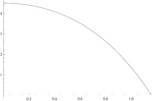
Figure 1: Numerical plot of the function $f(R)$ with integration constant $c\simeq 2.4998$. Note that $f(0)=9/2$ and $f(R)$ decreases monotonically to zero at $R=R_{0}$, where $R_{0}\simeq 1.16$.

We find that there exists a point $r_{0}>0$ with $f(r_{0})=0$ for the choice

$$c \simeq 2.4998~{}.$$ (4.65)

The resulting plot of the function $f(R)$, with $R=r^{3}$, is shown in Figure 1. Smaller values of $c$ lead to $f(R)$ remaining positive, while for $c>2.4998$ we find the numerics becomes highly unstable. Indeed, the numerics is slightly unstable near the zero of $f$ for $c=2.4998$. As a cross check that we really do have a zero, we note that at a zero of $f(R)$ we necessarily have

$$f^{\prime}(R_{0}) = -\frac{6\sqrt{1+R_{0}^{6}}}{R_{0}}~{}.$$ (4.66)

In Figure 2 we numerically plot the function $f^{\prime}(R)+\frac{6\sqrt{1+R^{6}}}{R}$, which should tend to zero at $R=R_{0}$.

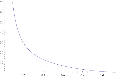
Figure 2: Numerical plot (with integration constant $c\simeq 2.4998$) of the function $f^{\prime}(R)+\frac{6\sqrt{1+R^{6}}}{R}$, which should tend to zero at $R=R_{0}\simeq 1.16$.

Of course, it is quite tantalizing that the numerical value of $c$ is so close to $5/2$, perhaps suggesting the possibility of an analytic solution, or at least an analytic explanation of $c=5/2$. We leave this question open.

5 Conclusions

The main result of this paper is the determination of the necessary and sufficient conditions on supersymmetric solutions of $D=11$ supergravity that are dual to ${\cal N}=2$ three-dimensional superconformal field theories. The eleven-dimensional metric is taken to be a warped product of AdS₄ with a seven-dimensional Riemannian metric, and we have allowed for the most general four-form $G$ consistent with $SO(3,2)$ symmetry. We showed that generically the supersymmetry conditions may be formulated in terms of a canonical local $SU(2)$-structure on the seven-dimensional manifold $Y_{7}$. The well-known Freund-Rubin AdS${}_{4}\times Y_{7}$ solutions where $Y_{7}$ is Sasaki-Einstein arise as a special case, characterized by an $SU(3)$-structure. For solutions with non-zero M2-brane charge, we showed that many geometrical and physical properties of $Y_{7}$ are captured by a contact structure, elaborating on the results presented in [26]. We also recovered the class of general solutions with vanishing M2-brane charge, previously discussed in [25].

By imposing a single additional requirement, that a certain vector bilinear is a Killing vector, we reduced the conditions to solving a second order non-linear ODE. The seven-dimensional metric on $Y_{7}$ is then fully specified by the choice of a (local) four-dimensional Kähler-Einstein metric, and any solution to this ODE. We managed to find an analytic solution of the ODE, and showed that this reproduces a class of solutions found originally in [21]. In addition, using a combination of analytic and numerical methods, we have discovered a further solution to our ODE, yielding a class of new supersymmetric AdS₄ solutions with non-trivial four-form flux. These can be interpreted as holographically dual to certain cubic superpotential deformations of ${\cal N}=2$ Chern-Simons gauge theories. When the Kähler-Einstein metric is chosen to be that on $\mathbb{CP}^{2}$, the seven-dimensional metric is a smooth (non-Einstein) metric on $S^{7}$, different from that of [21]. We suspect that there are no further regular solutions in this class.

Our work may be regarded as providing the foundation for studying more general aspects of ${\cal N}=2$ three-dimensional superconformal field theories with M-theory duals. For example, we expect that the geometric characterization of solutions we presented may be used to attack general problems, such as the gravity dual of ${\cal F}$-maximization, similarly to the developments in [29, 32]. It is also clear that using our results it will be possible to construct a consistent Kaluza-Klein truncation to four dimensions, extending that in [44]. The AdS₄ solutions dual to beta-deformations [45, 46] of ${\cal N}=2$ field theories must solve the equations that we presented, and it would interesting to verify this explicitly. Of course, it would also be very interesting to use our general equations as a method for finding new solutions (perhaps numerically), outside the classes that have been discovered so far. These are all exciting directions for future work.

Acknowledgments

We would like to thank the Isaac Newton Institute for hospitality. M. G. is supported by the ERC Starting Independent Researcher Grant 259133-ObservableString, D. M. is supported by the EPSRC Advanced Fellowship EP/D07150X/3, A. P. is supported by an A. G. Leventis Foundation grant and via the Act “Scholarship Programme of S. S. F. by the procedure of individual assessment, of 2011-12” by resources of the Operational Programme for Education and Lifelong Learning, of the European Social Fund (ESF) and of the NSRF, 2007-2013. D. M. also acknowledges partial support from the STFC grant ST/J002798/1. J. F. S. is supported by the Royal Society and Oriel College.

Appendix A Some useful identities

In this appendix we collect a number of useful identities that have been used repeatedly to derive the results presented in the main text.

From the algebraic equation in (2.1) one can derive the following useful identities

$$\left(\bar{\chi}_{i}^{c}\mathcal{C}\chi_{j}^{c}+\bar{\chi}_{i}\mathcal{C}\chi_{j}\right)-\frac{\mathrm{i}m}{3}\mathrm{e}^{-3\Delta}\bar{\chi}_{i}^{c}\mathcal{C}\chi_{j}~{}~{}~{}~{}~{}~{}~{}~{}~{}~{}~{}~{}~{}~{}~{}~{}~{}~{}~{}~{}~{}~{}~{}~{}~{}~{}~{}~{}~{}~{}~{}~{}~{}~{}~{}~{}~{}~{}~{}~{}~{}$$

$$+\frac{1}{2}\partial_{m}\Delta\bar{\chi}_{i}^{c}[\mathcal{C},\gamma^{m}]_{-}\chi_{j}+\frac{1}{288}F_{mnpq}\mathrm{e}^{-3\Delta}\bar{\chi}_{i}^{c}[\mathcal{C},\gamma^{mnpq}]_{+}\chi_{j} = 0~{},~{}~{}~{}~{}$$ (A.1)

$$\left(\bar{\chi}_{i}^{c}\mathcal{C}\chi_{j}^{c}-\bar{\chi}_{i}\mathcal{C}\chi_{j}\right)+\frac{1}{2}\partial_{m}\Delta\bar{\chi}_{i}^{c}[\mathcal{C},\gamma^{m}]_{+}\chi_{j}+\frac{1}{288}F_{mnpq}\mathrm{e}^{-3\Delta}\bar{\chi}_{i}^{c}[\mathcal{C},\gamma^{mnpq}]_{-}\chi_{j} = 0~{},$$ (A.2)

where $\mathcal{C}\in$ Cliff$(7)$ is an arbitrary element of the Clifford algebra and $[~{},~{}]_{\pm}$ denotes the (anti)-commutator. Similarly we note

$$\left(\bar{\chi}_{i}^{c}\mathcal{C}\chi_{j}-\bar{\chi}_{i}\mathcal{C}\chi_{j}^{c}\right)+\frac{\mathrm{i}m}{3}\mathrm{e}^{-3\Delta}\bar{\chi}_{i}\mathcal{C}\chi_{j}~{}~{}~{}~{}~{}~{}~{}~{}~{}~{}~{}~{}~{}~{}~{}~{}~{}~{}~{}~{}~{}~{}~{}~{}~{}~{}~{}~{}~{}~{}~{}~{}~{}~{}~{}~{}~{}~{}~{}~{}~{}$$

$$-\frac{1}{2}\partial_{m}\Delta\bar{\chi}_{i}[\mathcal{C},\gamma^{m}]_{-}\chi_{j}-\frac{1}{288}F_{mnpq}\mathrm{e}^{-3\Delta}\bar{\chi}_{i}[\mathcal{C},\gamma^{mnpq}]_{-}\chi_{j} = 0~{},~{}~{}~{}~{}$$ (A.3)

$$\left(\bar{\chi}_{i}^{c}\mathcal{C}\chi_{j}+\bar{\chi}_{i}\mathcal{C}\chi_{j}^{c}\right)+\frac{1}{2}\partial_{m}\Delta\bar{\chi}_{i}[\mathcal{C},\gamma^{m}]_{+}\chi_{j}+\frac{1}{288}F_{mnpq}\mathrm{e}^{-3\Delta}\bar{\chi}_{i}[\mathcal{C},\gamma^{mnpq}]_{+}\chi_{j} = 0~{}.$$ (A.4)

Similar identities exist in the alternative basis (2.12).

From the Fierz identity for the $\mathrm{Cliff(7)}$ algebra

$$\bar{\xi}_{1}\xi_{2}\,\bar{\xi}_{3}\xi_{4} = \frac{1}{8}\Bigg{[}\bar{\xi}_{1}\xi_{4}\,\bar{\xi}_{3}\xi_{2}+\bar{\xi}_{1}\gamma_{m}\xi_{4}\,\bar{\xi}_{3}\gamma^{m}\xi_{2}-\frac{1}{2!}\bar{\xi}_{1}\gamma_{mn}\xi_{4}\,\bar{\xi}_{3}\gamma^{mn}\xi_{2}$$ (A.5)

$$-\frac{1}{3!}\bar{\xi}_{1}\gamma_{mnp}\xi_{4}\,\bar{\xi}_{3}\gamma^{mnp}\xi_{2}\Bigg{]}~{},$$

where $\xi_{a}$, $a=1,2,3,4$, are arbitrary Spin(7) spinors, we derive the useful identity

$$\bar{\xi^{c}_{1}}\gamma^{m}\xi_{2}\,\bar{\xi^{c}_{2}}\gamma_{m}\xi_{4} = \bar{\xi^{c}_{1}}\xi_{4}\,\bar{\xi^{c}_{2}}\xi_{2}-\bar{\xi^{c}_{1}}\xi_{2}\,\bar{\xi^{c}_{2}}\xi_{4}~{}.$$ (A.6)

Appendix B $SU(2)$- and $SU(3)$-structures in dimension $d=7$

In the main text we have presented our results, summarized in the equations in section 2.6, in terms of an $SU(2)$-structure. This is defined by the three one-forms $E_{1}$, $E_{2}$, $E_{3}$, and three $SU(2)$-invariant two-forms $J_{1}$, $J_{2}$, $J_{3}$. In arguing that the conditions we write are sufficient, it is also convenient to think of this in terms two $SU(3)$-structures, defined by the Killing spinors $\chi_{\pm}$. In this appendix we present explicit formulas for the spinor bilinears in terms of both $SU(2)$- and $SU(3)$-structures.

B.1 $SU(2)$-structure

Recall that the $SU(2)$-structure is specified by two spinors $\chi_{1}$, $\chi_{2}$, or equivalently the linear combinations $\chi_{\pm}\equiv\frac{1}{\sqrt{2}}\left(\chi_{1}\pm\mathrm{i}\chi_{2}\right)$ defined in (2.12). Here we choose to use $\chi_{\pm}$ as our basis.

We then have the following zero-form bilinears

$$\bar{\chi}_{+}\chi_{+} = \bar{\chi}_{-}\chi_{-}\ =\ 1~{},$$

$$\bar{\chi}_{+}\chi_{-} = 0~{},$$

$$S \equiv \bar{\chi}_{+}^{c}\chi_{+}\ =\ (\bar{\chi}_{-}^{c}\chi_{-})^{*}~{},$$

$$\zeta \equiv \mathrm{i}\bar{\chi}_{+}^{c}\chi_{-}\ =\ \frac{m}{6}\mathrm{e}^{-3\Delta}~{},$$ (B.1)

one-form bilinears

$$K \equiv \mathrm{i}\bar{\chi}_{+}^{c}\gamma_{(1)}\chi_{-}\ =\ \|\xi\|E_{1}~{},$$

$$L \equiv \bar{\chi}_{-}\gamma_{(1)}\chi_{+}\ =\ \frac{S}{|S|}\left(\mathrm{i}\frac{|S|}{\|\xi\|}E_{1}+\sqrt{1-\|\xi\|^{2}}E_{2}-\mathrm{i}\frac{\zeta\sqrt{1-\|\xi\|^{2}}}{\|\xi\|}E_{3}\right)~{},$$

$$P \equiv -\bar{\chi}_{+}\gamma_{(1)}\chi_{+}\ =\ \bar{\chi}_{-}\gamma_{(1)}\chi_{-}\ =\ \frac{\zeta}{\|\xi\|}E_{1}+\frac{|S|\sqrt{1-\|\xi\|^{2}}}{\|\xi\|}E_{3}~{},$$ (B.2)

two-form bilinears

$$V_{\pm} \equiv \frac{1}{2\mathrm{i}}\left[\bar{\chi}_{+}\gamma_{(2)}\chi_{+}\pm\bar{\chi}_{-}\gamma_{(2)}\chi_{-}\right]~{},$$

$$V_{+} = \sqrt{1-\|\xi\|^{2}}J_{2}~{},$$

$$V_{-} = \zeta J_{3}+\frac{1}{\|\xi\|}E_{2}\wedge\left(|S|\sqrt{1-\|\xi\|^{2}}E_{1}-\zeta E_{3}\right)~{},$$

$$\bar{\chi}^{c}_{+}\gamma_{(2)}\chi_{-} = -J_{3}+\|\xi\|E_{2}\wedge E_{3}-\mathrm{i}\sqrt{1-\|\xi\|^{2}}J_{1}$$ (B.3)

and three-form bilinears

$$W_{\pm} \equiv \frac{1}{2}\left[\bar{\chi}_{+}^{c}\gamma_{(3)}\chi_{+}\pm\left(\bar{\chi}_{-}^{c}\gamma_{(3)}\chi_{-}\right)^{*}\right]~{},$$

$$\mathrm{Re}\,\left[\frac{|S|}{S}W_{-}\right] = -\sqrt{1-\|\xi\|^{2}}J_{3}\wedge E_{2},$$

$$\mathrm{Im}\,\left[\frac{|S|}{S}W_{-}\right] = -J_{3}\wedge\left(\frac{|S|}{\|\xi\|}E_{1}-\frac{\zeta\sqrt{1-\|\xi\|^{2}}}{\|\xi\|}E_{3}\right)+|S|E_{123}~{},$$

$$\mathrm{Re}\,\left[\frac{|S|}{S}W_{+}\right] = \frac{1}{\|\xi\|}J_{1}\wedge\left(|S|\sqrt{1-\|\xi\|^{2}}E_{1}-\zeta E_{3}\right)+\zeta J_{2}\wedge E_{2}~{},$$

$$\mathrm{Im}\,\left[\frac{|S|}{S}W_{+}\right] = -J_{1}\wedge E_{2}-\|\xi\|J_{2}\wedge E_{3}~{},$$

$$\mathrm{Im}\left[\bar{\chi}_{+}^{c}\gamma_{(3)}\chi_{-}\right] = |S|J_{2}\wedge E_{2}-\frac{1}{\|\xi\|}J_{1}\wedge(\zeta\sqrt{1-\|\xi\|^{2}}E_{1}+|S|E_{3})~{},$$

$$\mathrm{i}\bar{\chi}_{+}\gamma_{(3)}\chi_{+} = \|\xi\|J_{3}\wedge E_{1}-E_{123}+|S|J_{1}\wedge E_{2}$$ (B.4)

$$+\frac{1}{\|\xi\|}J_{2}\wedge\left(\zeta\sqrt{1-\|\xi\|^{2}}E_{1}+|S|E_{3}\right)~{}.$$

Notice that the two-forms and three-forms above are an incomplete list – we have included only those bilinears that are referred to explicitly in the text.

B.2 $SU(3)$-structures

Recall that we defined the two non-canonical $SU(3)$-structures as real vectors $\mathcal{K}_{\pm}\equiv\bar{\chi}_{\pm}\gamma_{(1)}\chi_{\pm}$, real two-forms $\mathcal{J}_{\pm}\equiv-\mathrm{i}\bar{\chi}_{\pm}\gamma_{(2)}\chi_{\pm}$, and complex three-forms $\Omega_{\pm}\equiv\bar{\chi}_{\pm}^{c}\gamma_{(3)}\chi_{\pm}$. Then we have the one-form bilinears

$$\mathcal{K}_{+} = -\mathcal{K}_{-}\ =\ -P~{},$$ (B.5)

two-form bilinears

$$\mathcal{J}_{\pm} = V_{+}\pm V_{-}~{},$$ (B.6)

and three-form bilinears

$$\Omega_{+} = W_{+}+W_{-}~{},\qquad\Omega_{-}\ =\ (W_{+}-W_{-})^{*}~{}.$$ (B.7)

Appendix C The Sasaki-Einstein case

In this appendix we study the case in which the three one-forms $K,\mathrm{Re}\,S^{*}L,\mathrm{Im}\,S^{*}L$ are linearly dependent. When they are linearly independent we have an $SU(2)$ structure, and in an open set we can then introduce corresponding coordinates, as described in section 2.5. Since these one-forms are derived from spinor bilinears, linear dependence implies we have an $SU(3)$ structure. Focusing on the $m\neq 0$ case for clarity, we will prove that the only solutions for which we have a global $SU(3)$ structure are Sasaki-Einstein.

In order to proceed, we impose the linear relation

$$aK+b\,\mathrm{Re}\,S^{*}L+c\,\mathrm{Im}\,S^{*}L = 0~{},$$ (C.1)

with $a$, $b$, $c$ not all zero. Making use of the Fierz identity in (A.6) it is straightforward to compute the dot products of each of $K,\mathrm{Re}\,S^{*}L,\mathrm{Im}\,S^{*}L$ into this equation. An analysis of the resulting three equations then implies that at least one of $|S|=0$ or $\|\xi\|=1$ must hold. In particular, if $|S|=0$ then necessarily $a=0$, while if $\|\xi\|=1$ then $a=c(\zeta^{2}-1)$. The following analysis then treats these cases in turn.

If $|S|=0$ then of course also $S=0$. The bilinear equation (2.25) then implies that $L=0$ and hence in particular that the one-form $\bar{\chi}_{1}\gamma_{(1)}\chi_{1}=0$. This says that $\chi_{1}$ defines a $G_{2}$ structure, rather than an $SU(3)$ structure, and hence that $\chi_{1}$ satisfies a reality (Majorana) condition $\chi_{1}=\mu\chi_{1}^{c}$. The scalar bilinears determine that $\mu=-\mathrm{i}/\zeta$, and since $|\mu|^{2}=1$ we conclude that $\zeta=1$ and the warp factor is constant $\mathrm{e}^{3\Delta}=m/6$. Finally, the bilinear equation (2.29) and its $\chi_{-}$ analogue imply

$$\mathrm{e}^{3\Delta}\star F = \mathrm{d}\left(\mathrm{i}\,\mathrm{e}^{6\Delta}\bar{\chi}_{1}\gamma_{(2)}\chi_{1}\right)-6\mathrm{e}^{6\Delta}\mathrm{Im}\left[\bar{\chi}_{1}^{c}\gamma_{(3)}\chi_{1}\right]~{},$$ (C.2)

which in turn immediately implies that $F=0$. This is because the Majorana condition $\chi_{1}=-\mathrm{i}\chi_{1}^{c}$ implies that the two-form bilinear $\bar{\chi}_{1}\gamma_{(2)}\chi_{1}=0$ (there are no $G_{2}$-invariant two-forms), while the three-form bilinear $\bar{\chi}_{1}^{c}\gamma_{(3)}\chi_{1}$ is real (corresponding to the unique $G_{2}$-invariant three-form). We conclude that the warp factor is constant and $F=0$, so that the Killing spinor equation for $\chi_{1}$ (2.1) leads to weak $G_{2}$ holonomy and hence an Einstein metric. The second Killing spinor $\chi_{2}$ (for which the analysis is essentially the same) then of course leads to a Sasaki-Einstein manifold.

Alternatively, if $\|\xi\|=1$ then we immediately have $\mathrm{Re}\,S^{*}L=0$ by computing the square length of the latter using (A.6). But since also $a=-c|S|^{2}$ follows from linear dependence, we also have the additional relation $\mathrm{Im}\,S^{*}L=|S|^{2}K$ from (C.1). There is thus only one linearly independent vector, as one expects since we must have an $SU(3)$ structure. Using the exterior derivatives of the one-form bilinears one can then show that where $S$ is non-zero we have that $K$ is closed, $\mathrm{d}K=0$ (recall that $K$ is Killing in any case, so this implies that $K$ is parallel). By contracting $K$ into the bilinear equation for $\mathrm{d}K$ and making use of a Fierz identity one then proves that $\mathrm{d}\Delta=0$. Given that $\|\xi\|^{2}=|S|^{2}+\zeta^{2}=1$ by assumption, this immediately implies that $S$ is constant, and hence that $L=0$. But then all vectors are identically zero, and we have a contradiction. Thus it must be that $S=0$ and we hence reduce to the previous case, which implies that $Y_{7}$ is Sasaki-Einstein with $F=0$ and $\Delta$ constant.

Appendix D The case $m=0$, $\mathrm{Im}\left[\bar{\chi}_{1}\chi_{2}\right]\neq 0$

In section 2.2 we noted that when $m=0$ we can no longer conclude that equation (2.15) holds. In this appendix we study the case $m=0$ but $\mathrm{Im}\left[\bar{\chi}_{1}\chi_{2}\right]$ not being identically zero, in particular showing that there are no regular solutions in this class. Note this is different from the class of $m=0$ geometries discussed in section 2.7, and cannot be obtained by taking the $m\rightarrow 0$ limit of the general $m\neq 0$ equations in the main text.

We begin by defining

$$h \equiv \mathrm{Im}\left[\bar{\chi}_{1}\chi_{2}\right]~{},$$ (D.1)

which is a function on $Y_{7}$. Equation (2.19) now becomes

$$\mathrm{Im}\,K = \frac{1}{2}\mathrm{d}h~{},$$ (D.2)

while the imaginary part of equation (2.20) reads

$$\nabla_{(m}(\mathrm{Im}\,K)_{n)} = -2hg_{7\,mn}~{}.$$ (D.3)

Combining the last two equations gives

$$\nabla_{m}\nabla_{n}h = -t^{2}hg_{7\,mn}~{},$$ (D.4)

where $t=2$. Notice that $\mathrm{Im}\,K$ is a particular type of gradient conformal Killing vector. Equation (D.4) was studied by Obata in [43]. In particular, he proved that if a complete Riemannian manifold of dimension $d\geq 2$ admits a non-constant function $h$ satisfying (D.4), where $t$ is (without loss of generality) a positive constant, then it is necessarily isometric to a round sphere of radius $1/t$. Thus we immediately conclude that if $h$ is not identically zero, $Y_{7}$ is isometric to the round $S^{7}$ with radius $1/2$.

Now as in section 2.7, the Bianchi identity and equation of motion for $F$ imply that $F$ is harmonic on the conformally rescaled manifold $(Y_{7},\tilde{g}_{7})$, where $\tilde{g}_{7}=\mathrm{e}^{-6\Delta}g_{7}$. But in the case at hand, $Y_{7}=S^{7}$ and the Hodge theorem implies there are no harmonic four-forms since $H^{4}(S^{7};\mathbb{R})=0$. Thus for a non-singular solution in fact $F=0$, and hence the M-theory four-form $G=0$. The equation of motion (2.1) then implies that the eleven-dimensional spacetime must be Ricci-flat, but this is a contradiction.

References

- [1] J. M. Maldacena, “The Large limit of superconformal field theories and supergravity,” Adv. Theor. Math. Phys. 2, 231 (1998) [hep-th/9711200].
- [2] D. Martelli and J. Sparks, “-structures, fluxes and calibrations in M theory,” Phys. Rev. D 68, 085014 (2003) [arXiv:hep-th/0306225].
- [3] J. P. Gauntlett, D. Martelli, J. Sparks and D. Waldram, “Supersymmetric AdS5 solutions of M-theory,” Class. Quant. Grav. 21, 4335 (2004) [hep-th/0402153].
- [4] H. Lin, O. Lunin and J. M. Maldacena, “Bubbling AdS space and 1/2 BPS geometries,” JHEP 0410, 025 (2004) [hep-th/0409174].
- [5] D. Lust and D. Tsimpis, “Supersymmetric AdS4 compactifications of IIA supergravity,” JHEP 0502, 027 (2005) [hep-th/0412250].
- [6] J. P. Gauntlett, D. Martelli, J. Sparks and D. Waldram, “Supersymmetric AdS5 solutions of type IIB supergravity,” Class. Quant. Grav. 23, 4693 (2006) [hep-th/0510125].
- [7] E. O Colgain, J. -B. Wu and H. Yavartanoo, “On the generality of the LLM geometries in M-theory,” JHEP 1104, 002 (2011) [arXiv:1010.5982 [hep-th]].
- [8] J. P. Gauntlett, D. Martelli, S. Pakis and D. Waldram, “structures and wrapped NS5-branes,” Commun. Math. Phys. 247, 421 (2004) [hep-th/0205050].
- [9] A. Lukas and P. M. Saffin, “M theory compactification, fluxes and AdS4,” Phys. Rev. D 71, 046005 (2005) [arXiv:hep-th/0403235].
- [10] K. Behrndt, M. Cvetic and T. Liu, “Classification of supersymmetric flux vacua in M-theory,” Nucl. Phys. B 749, 25 (2006) [arXiv:hep-th/0512032].
- [11] J. Bagger and N. Lambert, “Modeling Multiple M2’s,” Phys. Rev. D75, 045020 (2007) [hep-th/0611108].
- [12] A. Gustavsson, “Algebraic structures on parallel M2-branes,” Nucl. Phys. B811 (2009) 66-76 [arXiv:0709.1260 [hep-th]].
- [13] O. Aharony, O. Bergman, D. L. Jafferis and J. Maldacena, “ superconformal Chern-Simons-matter theories, M2-branes and their gravity duals,” JHEP 0810, 091 (2008) [arXiv:0806.1218 [hep-th]].
- [14] A. Kapustin, B. Willett and I. Yaakov, “Exact Results for Wilson Loops in Superconformal Chern-Simons Theories with Matter,” JHEP 1003, 089 (2010) [arXiv:0909.4559 [hep-th]].
- [15] D. L. Jafferis, “The Exact Superconformal R-Symmetry Extremizes ,” JHEP 1205, 159 (2012) [arXiv:1012.3210 [hep-th]].
- [16] N. Hama, K. Hosomichi and S. Lee, “Notes on SUSY Gauge Theories on Three-Sphere,” JHEP 1103, 127 (2011). [arXiv:1012.3512 [hep-th]].
- [17] D. Martelli and J. Sparks, “The large limit of quiver matrix models and Sasaki-Einstein manifolds,” Phys. Rev. D 84, 046008 (2011) [arXiv:1102.5289 [hep-th]].
- [18] S. Cheon, H. Kim and N. Kim, “Calculating the partition function of Gauge theories on and AdS/CFT correspondence,” JHEP 1105, 134 (2011) [arXiv:1102.5565 [hep-th]].
- [19] D. L. Jafferis, I. R. Klebanov, S. S. Pufu and B. R. Safdi, “Towards the F-Theorem: Field Theories on the Three-Sphere,” JHEP 1106, 102 (2011) [arXiv:1103.1181 [hep-th]].
- [20] A. Amariti and S. Franco, “Free Energy vs Sasaki-Einstein Volume for Infinite Families of M2-Brane Theories,” arXiv:1204.6040 [hep-th].
- [21] R. Corrado, K. Pilch and N. P. Warner, “An supersymmetric membrane flow,” Nucl. Phys. B 629, 74 (2002) [arXiv:hep-th/0107220].
- [22] I. Klebanov, T. Klose and A. Murugan, “AdS4/CFT3 – Squashed, Stretched and Warped,” JHEP 0903, 140 (2009) [arXiv:0809.3773 [hep-th]].
- [23] C. Ahn and K. Woo, “The Gauge Dual of A Warped Product of AdS4 and A Squashed and Stretched Seven-Manifold,” Class. Quant. Grav. 27, 035009 (2010) [arXiv:0908.2546 [hep-th]].
- [24] C. Ahn, “The Eleven-Dimensional Uplift of Four-Dimensional Supersymmetric RG Flow,” J. Geom. Phys. 62, 1480 (2012) [arXiv:0910.3533 [hep-th]].
- [25] J. P. Gauntlett, O. A. P. Mac Conamhna, T. Mateos and D. Waldram, “AdS spacetimes from wrapped M5 branes,” JHEP 0611, 053 (2006) [hep-th/0605146].
- [26] M. Gabella, D. Martelli, A. Passias and J. Sparks, “The free energy of N=2 supersymmetric AdS4 solutions of M-theory,” JHEP 1110, 039 (2011) [arXiv:1107.5035 [hep-th]].
- [27] N. Halmagyi, K. Pilch and N. P. Warner, “On Supersymmetric Flux Solutions of M-theory,” arXiv:1207.4325 [hep-th].
- [28] J. P. Gauntlett and S. Pakis, “The Geometry of Killing spinors,” JHEP 0304, 039 (2003) [hep-th/0212008].
- [29] M. Gabella, J. P. Gauntlett, E. Palti, J. Sparks and D. Waldram, “AdS5 Solutions of Type IIB Supergravity and Generalized Complex Geometry,” Commun. Math. Phys. 299, 365 (2010) [arXiv:0906.4109 [hep-th]].
- [30] M. Pernici and E. Sezgin, “Spontaneous compactification of seven-dimensional supergravity theories,” Class. Quant. Grav. 2 (1985) 673.
- [31] R. Emparan, C. V. Johnson and R. C. Myers, “Surface terms as counterterms in the AdS/CFT correspondence,” Phys. Rev. D 60, 104001 (1999) [arXiv:hep-th/9903238].
- [32] M. Gabella and J. Sparks, “Generalized Geometry in AdS/CFT and Volume Minimization,” Nucl. Phys. B 861, 53 (2012) [arXiv:1011.4296 [hep-th]].
- [33] D. Conti and S. Salamon “Generalized Killing spinors in dimension 5” Trans. Amer. Math. Soc. 359 (2007), no. 11, 5319-5343 [arXiv:math/0508375].
- [34] L. Bedulli and L. Vezzoni “Torsion of structures and Ricci curvature in dimension 5” arXiv:math/0702790 [math.DG].
- [35] D. Berenstein, C. P. Herzog and I. R. Klebanov, “Baryon spectra and AdS/CFT correspondence,” JHEP 0206, 047 (2002) [arXiv:hep-th/0202150].
- [36] I. R. Klebanov, S. S. Pufu and T. Tesileanu, “Membranes with Topological Charge and AdS4/CFT3 Correspondence,” Phys. Rev. D 81, 125011 (2010) [arXiv:1004.0413 [hep-th]].
- [37] N. Benishti, D. Rodriguez-Gomez and J. Sparks, “Baryonic symmetries and M5 branes in the AdS4/CFT3 correspondence,” JHEP 1007, 024 (2010) [arXiv: 1004.2045 [hep-th]].
- [38] O. Barwald, N. D. Lambert and P. C. West, “A Calibration bound for the M theory five-brane,” Phys. Lett. B 463, 33 (1999) [arXiv:hep-th/9907170].
- [39] M. Cvetic, H. Lu, D. N. Page and C. N. Pope, “New Einstein-Sasaki spaces in five and higher dimensions,” Phys. Rev. Lett. 95, 071101 (2005) [hep-th/0504225].
- [40] D. Martelli and J. Sparks, “Toric Sasaki-Einstein metrics on ,” Phys. Lett. B 621, 208 (2005) [hep-th/0505027].
- [41] J. P. Gauntlett, D. Martelli, J. Sparks and S. -T. Yau, “Obstructions to the existence of Sasaki-Einstein metrics,” Commun. Math. Phys. 273, 803 (2007) [hep-th/0607080].
- [42] D. Martelli, J. Sparks and S. -T. Yau, “Sasaki-Einstein manifolds and volume minimisation,” Commun. Math. Phys. 280, 611 (2008) [hep-th/0603021].
- [43] M. Obata, “Certain conditions for a Riemannian manifold to be isometric with a sphere,” J. Math. Soc. Japan 14 (1962) 333-340.
- [44] J. P. Gauntlett and O. Varela, “Consistent Kaluza-Klein reductions for general supersymmetric AdS solutions,” Phys. Rev. D 76, 126007 (2007) [arXiv:0707.2315 [hep-th]].
- [45] O. Lunin and J. M. Maldacena, “Deforming field theories with global symmetry and their gravity duals,” JHEP 0505, 033 (2005) [hep-th/0502086].
- [46] J. P. Gauntlett, S. Lee, T. Mateos and D. Waldram, “Marginal deformations of field theories with AdS4 duals,” JHEP 0508, 030 (2005) [hep-th/0505207].
- [47] B. Kol, “On conformal deformations,” JHEP 0209, 046 (2002) [hep-th/0205141].