Condition Numbers of Indefinite Rank $2$ Ghost Wishart Matrices

Abstract

We define an indefinite Wishart matrix as a matrix of the form $A=W^{T}W\Sigma$, where $\Sigma$ is an indefinite diagonal matrix and $W$ is a matrix of independent standard normals. We focus on the case where $W$ is $L\times 2$ which has engineering applications. We obtain the distribution of the ratio of the eigenvalues of $A$. This distribution can be “folded” to give the distribution of the condition number. We calculate formulas for $W$ real $\left(\beta=1\right)$, complex $\left(\beta=2\right)$, quaternionic $\left(\beta=4\right)$ or any ghost $0<\beta<\infty$. We then corroborate our work by comparing them against numerical experiments.

Department of Mathematics, Massachusetts Institute of Technology, Cambridge MA, 02139

Problem Statement

Let $W$ be an $L\times 2$ matrix whose elements are drawn from a normal distribution. Let the two real eigenvalues of $A=W^{T}W\Sigma$ be denoted by $\lambda_{1}$ and $\lambda_{2}$. The condition number of $A$ is $\sigma=\frac{\left|\underset{}{\lambda_{\mbox{max}}}\right|}{\left|\lambda_{\mbox{min}}\right|}$, where $\left|\lambda_{\mbox{max}}\right|=\mbox{max}\left(\left|\lambda_{1}\right|,\left|\lambda_{2}\right|\right)$ and $\left|\lambda_{\mbox{min}}\right|=\mbox{min}\left(\left|\lambda_{1}\right|,\left|\lambda_{2}\right|\right)$. What is the condition number distribution of $A=W^{T}W\Sigma$, where $\Sigma=\left[\begin{array}[]{cc}x_{1}\\ &x_{2}\end{array}\right]$ is full rank with $\mbox{sgn}\left(x_{2}\right)=-\mbox{sgn}\left(x_{1}\right)$? Though much is known when $\Sigma$ is positive definite [5], to the extent of our knowledge, the indefinite case is rarely considered. We work out the distribution of the ratio of the eigenvalues and the condition number of $A$ as it has applications in hypersensitive ground based radars [1, 2].

A ghost $\beta-$normal is a construction that works in many ways like a real $\left(\beta=1\right)$, complex $\left(\beta=2\right)$, and quaternionic $\left(\beta=4\right)$ standard normal [6]. In particular, its absolute value has a $\chi_{\beta}$ distribution on $\left[0,\infty\right)$ . In general, we allow $W$ to be an $L\times 2$ matrix sampled from a $\beta-$normal distribution but we immediately turn this into a problem involving real matrices namely the condition number of $R\Sigma R^{T}$, where $R\sim\left[\begin{array}[]{cc}\chi_{L\beta}&\chi_{\beta}\\ &\chi_{(L-1)\beta}\end{array}\right]$.

Distribution of the Ratio of the Eigenvalues

We first write $W=QR$, where $Q$ is an $L\times 2$ orthogonal matrix and $R$ is an $2\times 2$ upper triangular matrix [3, reduced QR factorization]. Note that $W\Sigma W^{T}=QR\Sigma R^{T}Q^{T}$ and that $A$ is similar to $R\Sigma R^{T}$. The elements of $R$ may be chosen to be non-negative in which case it is well known that they have independent $\chi$-distributions

$$R\equiv\left[\begin{array}[]{cc}a&b\\ &c\end{array}\right]\sim\left[\begin{array}[]{cc}\chi_{L\beta}&\chi_{\beta}\\ &\chi_{(L-1)\beta}\end{array}\right]$$ (1)

and that [5]

$$\chi_{k}\sim\frac{x^{k-1}e^{-x^{2}/2}}{2^{k/2-1}\Gamma(k/2)},\quad x\geq 0$$ (2)

where $k$ denotes degrees of freedom and $\beta=1$ corresponds to entries being real, $\beta=2$ complex, $\beta=4$ quaternionic and general $\beta$ for any ghost [6]. The positivity of $R_{1,2}$ merits some comment as it does not generalize well beyond two columns. With two columns, even for $\beta\neq 1$, a phase can be pulled out of the rows and columns of $R$ and absorbed elsewhere without any loss of generality.

Comment: The concept of a $QR$ decomposition is often sensible for $W$’s with entries drawn from $\beta-$normal distribution. As with reals, complex, and quaternions, $R$ can be chosen to have positive diagonal elements for rank $2$ matrices, and $R_{12}$ can be chosen non-negative as well, by absorbing "phases" or unit-ghosts either into $Q$ or $R\Sigma R^{T}$.

This argument follows the ghost methodology described in [6]. However, mathematically the point of departure can be the computation of the condition number distribution for the real matrix $R\Sigma R^{T}$ without any mention of the ghosts or their interpretation.

The joint distribution of the elements $a,b,c$ of $R$ with parameters $L$ and $\beta$ is:

$$\rho_{R}\left(a,b,c;L,\beta\right)=\frac{2^{-\beta L+3}a^{\beta L-1}b^{\beta-1}c^{\beta\left(L-1\right)-1}\exp\left[-\frac{1}{2}\left(a^{2}+b^{2}+c^{2}\right)\right]}{\Gamma\left(\frac{\beta L}{2}\right)\Gamma\left(\frac{\beta}{2}\right)\Gamma\left[\frac{\beta}{2}\left(L-1\right)\right]};$$ (3)

in particular

$$\rho_{R}\left(a,b,c;L,\beta=1\right) = \frac{2a^{L-1}c^{L-2}\exp\left[-\frac{1}{2}\left(a^{2}+b^{2}+c^{2}\right)\right]}{\pi\Gamma\left(L-1\right)},$$

$$\rho_{R}\left(a,b,c;L,\beta=2\right) = \frac{2^{-2L+3}\left(L-1\right)a^{2L-1}bc^{2L-3}\exp\left[-\frac{1}{2}\left(a^{2}+b^{2}+c^{2}\right)\right]}{\Gamma^{2}\left(L\right)},$$

$$\rho_{R}\left(a,b,c;L,\beta=4\right) = \frac{2^{-4\left(L-1\right)}\left(L-1\right)\left(2L-1\right)a^{4L-1}b^{3}c^{4L-5}\exp\left[-\frac{1}{2}\left(a^{2}+b^{2}+c^{2}\right)\right]}{\Gamma^{2}\left(2L\right)}\mbox{ }.$$

The first change of variables computes the matrix whose condition number we are seeking, $R\Sigma R^{T}$ as: $R\left[\begin{array}[]{cc}x_{1}\\ &x_{2}\end{array}\right]R^{T}=\left[\begin{array}[]{cc}a^{2}x_{1}+b^{2}x_{2}&bcx_{2}\\ bcx_{2}&c^{2}x_{2}\end{array}\right]\equiv\left[\begin{array}[]{cc}d&f\\ f&e\end{array}\right]$. From Eq. (1) we see that $a,b,c$ are real and non-negative. The old and new variables are related by

$$c=\sqrt{e/x_{2}},\qquad b=\frac{f}{x_{2}\sqrt{e/x_{2}}},\qquad a=\sqrt{\frac{1}{x_{1}}\left(d-\frac{f^{2}}{e}\right)}.$$ (4)

Note that $c>0$ implies $\mbox{sgn}\left(e\right)=\mbox{sgn}\left(x_{2}\right)$ and $f=bcx_{2}\Rightarrow\mbox{sgn}\left(f\right)=\mbox{sgn}\left(x_{2}\right)$. The Jacobian associated with this transformation is $\left|\frac{\partial(a,b,c)}{\partial(d,e,f)}\right|=\left|\frac{1}{4ac^{2}x_{1}x_{2}^{2}}\right|$.

We make the eigenvalue decomposition of the symmetric matrix

$$\left[\begin{array}[]{cc}d&f\\ f&e\end{array}\right]\equiv\left[\begin{array}[]{cc}\cos\theta&-\sin\theta\\ \sin\theta&\cos\theta\end{array}\right]\left[\begin{array}[]{cc}\lambda_{1}\\ &\lambda_{2}\end{array}\right]\left[\begin{array}[]{cc}\cos\theta&\sin\theta\\ -\sin\theta&\cos\theta\end{array}\right],\quad\theta\in\left[0,\frac{\pi}{2}\right];$$ (5)

implying

$$d = \lambda_{1}\cos^{2}\theta+\lambda_{2}\sin^{2}\theta$$ (6)

$$e = \lambda_{1}\sin^{2}\theta+\lambda_{2}\cos^{2}\theta$$ (7)

$$f = \frac{\mbox{sin}2\theta}{2}\left(\lambda_{1}-\lambda_{2}\right).$$ (8)

The Jacobian associated with this transformation is $\left|\frac{\partial\left(d,e,f\right)}{\partial\left(\lambda_{1},\lambda_{2},\theta\right)}\right|=|\lambda_{1}-\lambda_{2}|$. The choice of $\theta\in\left[0,\frac{\pi}{2}\right]$ nails down the ordering of the eigenvalues

$$\begin{array}[]{ccccc}x_{2}<0<x_{1}&\Rightarrow&f<0&\Rightarrow&\lambda_{1}<0<\lambda_{2}\\ x_{1}<0<x_{2}&\Rightarrow&f>0&\Rightarrow&\lambda_{2}<0<\lambda_{1}.\end{array}$$ (9)

In summary, given $\theta\in\left[0,\frac{\pi}{2}\right]$, the constraints on $d,e,f$ are

$$\begin{array}[]{ccccc}x_{2}<0<x_{1}&\Rightarrow&d>\frac{f^{2}}{e},\mbox{ }e<0,\mbox{ }f<0,&\Rightarrow&\lambda_{1}<0<\lambda_{2}\\ x_{1}<0<x_{2}&\Rightarrow&d<\frac{f^{2}}{e},\mbox{ }e>0,\mbox{ }f>0&\Rightarrow&\lambda_{2}<0<\lambda_{1}.\end{array}$$

Intersecting $t\equiv-\frac{\lambda_{2}}{\lambda_{1}}\geq 0$ with the constraint space, we obtain

$$\tan^{2}\theta>t.$$ (10)

It is easy to see this is required by Eq. (7). Conversely given $\mbox{sgn}\left(e\right)=\mbox{sgn}\left(x_{2}\right)$ and $\tan^{2}\theta>t=-\frac{\lambda_{2}}{\lambda_{1}}$ we can solve for $d$ and $f$ so that $d,e$ and $f$ meet all of the constraints.

The next change of variables is to write the distribution as a ratio of the eigenvalues, i.e., $u=\lambda_{1},\>t=\frac{-\lambda_{2}}{\lambda_{1}},$ and $\theta$. The Jacobian associated with this transformation is $\left|\frac{\partial\left(\lambda_{1},\lambda_{2},\theta\right)}{\partial\left(u,t,\theta\right)}\right|=\left|u\right|$. Since we are interested in the condition number, we integrate $u$ over $\left\{\begin{array}[]{ccc}\left[0,\infty\right)&:&x_{2}>0\\ \left[0,-\infty\right)&:&x_{2}<0\end{array}\right.\;$, while applying the constraint (10)

$$\rho\left(t,\theta;L,\beta\right)=\left|\frac{2\left(-x_{1}x_{2}\right)^{\frac{\beta L}{2}}\Gamma\left(\beta L\right)t^{\frac{\beta L}{2}-1}\left(t+1\right)^{\beta}}{\Gamma\left(\frac{\beta}{2}\right)\Gamma\left[\frac{\beta}{2}\left(L-1\right)\right]\Gamma\left(\frac{\beta L}{2}\right)}\frac{\left(\sin\theta\cos\theta\right)^{\beta-1}\left[t\cos^{2}\theta-\sin^{2}\theta\right]^{\beta(L-1)}}{\left[x_{1}\left(t^{2}\cos^{2}\theta+\sin^{2}\theta\right)-x_{2}t\right]^{\beta L}}\right|,$$ (11)

where here and below implicitly $x_{1}$ and $x_{2}$ are parameters as well. This in the special cases reads

$$\rho\left(t,\theta;L,\beta=1\right) = \frac{2\left(-x_{1}x_{2}\right)^{L/2}\Gamma\left(L\right)t^{\frac{L}{2}-1}\left(t+1\right)}{\sqrt{\pi}\Gamma\left(\frac{L}{2}\right)\Gamma\left[\frac{1}{2}\left(L-1\right)\right]}\left|\frac{\left[t\cos^{2}\theta-\sin^{2}\theta\right]^{L-1}}{\left[x_{1}\left(t^{2}\cos^{2}\theta+\sin^{2}\theta\right)-x_{2}t\right]^{L}}\right|$$

$$\rho\left(t,\theta;L,\beta=2\right) = \frac{\left(-x_{1}x_{2}\right)^{L}\Gamma\left(2L\right)t^{L-1}\left(t+1\right)^{2}}{\Gamma\left(L-1\right)\Gamma\left(L\right)}\frac{\mbox{sin}2\theta\left[t\cos^{2}\theta-\sin^{2}\theta\right]^{2(L-1)}}{\left[x_{1}\left(t^{2}\cos^{2}\theta+\sin^{2}\theta\right)-x_{2}t\right]^{2L}}$$

$$\rho\left(t,\theta;L,\beta=4\right) = \frac{\left(-x_{1}x_{2}\right)^{2L}\Gamma\left(4L\right)t^{2L-1}\left(t+1\right)^{4}}{4\Gamma\left[2\left(L-1\right)\right]\Gamma\left(2L\right)}\frac{\mbox{sin}^{3}2\theta\left[t\cos^{2}\theta-\sin^{2}\theta\right]^{4(L-1)}}{\left[x_{1}\left(t^{2}\cos^{2}\theta+\sin^{2}\theta\right)-x_{2}t\right]^{4L}}.$$

Lastly we integrate $\theta$ from $\left[0,\pi/2\right]$ to obtain the distribution corresponding to the absolute value of the ratio of the eigenvalues $\rho\left(t;L,\beta\right)$. We denote the density after integrating $\theta$ with the same symbol $\rho$ without any confusion. In terms of the Gauss hypergeometric function [7], ${}_{2}F_{1}\left(a,b;c;z\right)$ we obtain,

$$\rho(t;L,\beta) = \frac{2^{\beta L-1}\left(-x_{1}x_{2}\right)^{\frac{\beta L}{2}}\Gamma\left(\frac{\beta L}{2}+\frac{1}{2}\right)\Gamma\left[\beta\left(L-1\right)+1\right]\left(t+1\right)^{\beta}t^{\frac{\beta L}{2}-\frac{\beta}{2}-1}}{\sqrt{\pi}\Gamma\left[\frac{\beta}{2}\left(L-1\right)\right]\Gamma\left(\beta L-\frac{\beta}{2}+1\right)\left|tx_{2}-x_{1}\right|^{\beta L}}\left(\frac{x_{1}-tx_{2}}{tx_{1}-x_{2}}\right)^{\beta L}$$

$$\times {}_{2}F_{1}\left(\beta L,\frac{\beta}{2};\beta L-\frac{\beta}{2}+1;\frac{x_{1}-tx_{2}}{x_{2}-tx_{1}}\right).$$

In particular,

$$\rho\left(t;L,\beta=1\right) = \frac{2^{L-1}(-x_{1}x_{2})^{L/2}\Gamma\left(\frac{1}{2}(L+1)\right)\Gamma\left(L\right)\left(t+1\right)t^{\frac{L}{2}-\frac{3}{2}}}{\sqrt{\pi}\Gamma\left(\frac{1}{2}\left(L-1\right)\right)\Gamma\left(L+\frac{1}{2}\right)\left|tx_{2}-x_{1}\right|^{L}}\left(\frac{x_{1}-tx_{2}}{tx_{1}-x_{2}}\right)^{L}$$

$$\times {}_{2}F_{1}\left(L,\frac{1}{2};L+\frac{1}{2};\frac{x_{1}-tx_{2}}{x_{2}-tx_{1}}\right),$$

$$\rho\left(t;L,\beta=2\right) = \frac{2^{2\left(L-1\right)}\left(x_{1}t-x_{2}\right)\left(-x_{1}x_{2}\right)^{L}\Gamma\left(L-\frac{1}{2}\right)\left(t+1\right)t^{L-2}}{\sqrt{\pi}\Gamma\left(L-1\right)\left(x_{1}-x_{2}\right)\left(tx_{2}-x_{1}\right)^{2L}}\left(\frac{x_{1}-tx_{2}}{tx_{1}-x_{2}}\right)^{2L},$$

$$\rho\left(t;L,\beta=4\right) = \frac{2^{4L-1}(-x_{1}x_{2})^{2L}\Gamma\left(2L+\frac{1}{2}\right)\Gamma\left(4L-3\right)\left(t+1\right)^{4}t^{2L-3}}{\sqrt{\pi}\Gamma\left[2\left(L-1\right)\right]\Gamma\left(4L-1\right)\left(tx_{2}-x_{1}\right)^{4L}}\left(\frac{x_{1}-tx_{2}}{tx_{1}-x_{2}}\right)^{4L}$$

$$\times {}_{2}F_{1}\left(4L,2;4L-1;\frac{x_{1}-tx_{2}}{x_{2}-tx_{1}}\right).$$

Distribution of the Condition Number

We can turn $\rho\left(t;L,\beta\right)$ to the condition number distribution by “folding” the distribution about one, i.e., take $\sigma\equiv\max\left(t,\frac{1}{t}\right)$. Therefore by folding the answer about one we can form the true condition number distribution from $\rho(t;L,\beta)$. Mathematically,

$$1=\int_{0}^{+\infty}dt\rho(t;L,\beta) = \int_{0}^{1}dt\rho\left(t;L,\beta\right)+\int_{1}^{\infty}dt\rho\left(t;L,\beta\right)\overset{\sigma\rightarrow\frac{1}{t}}{=}\int_{1}^{\infty}d\sigma\left(\frac{1}{\sigma^{2}}\rho\left(\frac{1}{\sigma};L,\beta\right)+\rho(\sigma;L,\beta)\right)$$

$$\equiv \int_{1}^{\infty}d\sigma f(\sigma;L,\beta)$$

This way we arrive at the desired distribution function, $f\left(\sigma,L,\beta\right)$, for the condition number of the indefinite Wishart matrices

$$f\left(\sigma;L,\beta\right)\equiv\frac{1}{\sigma^{2}}\rho\left(\frac{1}{\sigma};L,\beta\right)+\rho\left(\sigma;L,\beta\right),$$ (13)

where $\rho$ is as in Eq. (Distribution of the Ratio of the Eigenvalues).

The condition number distribution written explicitly is

$$f\left(\sigma;L,\beta\right) = \frac{2^{\beta L-1}\left(-x_{1}x_{2}\right)^{\frac{\beta L}{2}}\Gamma\left(\frac{\beta L}{2}+\frac{1}{2}\right)\Gamma\left[\beta\left(L-1\right)+1\right]\left(\sigma+1\right)^{\beta}\sigma^{\frac{\beta L}{2}-\frac{\beta}{2}-1}}{\sqrt{\pi}\Gamma\left[\frac{\beta}{2}\left(L-1\right)\right]\Gamma\left(\beta L-\frac{\beta}{2}+1\right)}$$

$$\times \left[{\scriptstyle\left|\frac{1}{\sigma x_{1}-x_{2}}\right|^{\beta L}{}_{2}F_{1}\left(\beta L,\frac{\beta}{2};\beta L-\frac{\beta}{2}+1;r\right)+\left|\frac{1}{\sigma x_{2}-x_{1}}\right|^{\beta L}{}_{2}F_{1}\left(\beta L,\frac{\beta}{2};\beta L-\frac{\beta}{2}+1;\frac{1}{r}\right)}\right]$$

where $$r\equiv\frac{\sigma x_{2}-x1}{\sigma x_{1}-x_{2}},\qquad\sigma=\left[1,\infty\right).$$

In particular,

$$f\left(\sigma;L,\beta=1\right) = \frac{2^{L-1}(-x_{1}x_{2})^{L/2}\Gamma\left(\frac{L}{2}+\frac{1}{2}\right)\Gamma\left(L\right)(\sigma+1)\sigma^{\frac{1}{2}L-\frac{3}{2}}}{\sqrt{\pi}\Gamma\left(\frac{L}{2}-\frac{1}{2}\right)\Gamma\left(\frac{1}{2}+L\right)}$$

$$\times \left[{\scriptstyle\left|\frac{1}{x_{2}-\sigma x_{1}}\right|^{L}{}_{2}F_{1}\left(\frac{1}{2},L;L+\frac{1}{2};r\right)+\left|\frac{1}{\sigma x_{2}-x_{1}}\right|^{L}{}_{2}F_{1}\left(\frac{1}{2},L;L+\frac{1}{2};\frac{1}{r}\right)}\right],$$

$$f\left(\sigma;L,\beta=2\right) = \frac{1}{4}\frac{(-4x_{1}x_{2})^{L}\Gamma(L-\frac{1}{2})(\sigma+1)}{\sqrt{\pi}(x_{1}-x_{2})\Gamma(L-1)\sigma^{4}}\left[\frac{\sigma^{L+2}(\sigma x_{1}-x_{2})}{(x_{2}-x_{1}\sigma)^{2L}}+\frac{\sigma^{L+2}(x_{1}-\sigma x_{2})}{(x_{2}\sigma-x_{1})^{2L}}\right],$$ (16)

$$f\left(\sigma;L,\beta=4\right) = \frac{2^{4L-1}\left(-x_{1}x_{2}\right)^{2L}\Gamma\left(2L+\frac{1}{2}\right)\Gamma\left[4\left(L-1\right)+1\right]\left(\sigma+1\right)^{4}\sigma^{2L-3}}{\sqrt{\pi}\Gamma\left[2\left(L-1\right)\right]\Gamma\left(4L-1\right)}$$

$$\times \left[{\scriptstyle\left(\frac{1}{\sigma x_{1}-x_{2}}\right)^{4L}{}_{2}F_{1}\left(4L,2;4L-1;r\right)+\left(\frac{1}{\sigma x_{2}-x_{1}}\right)^{4L}{}_{2}F_{1}\left(4L,2;4L-1;\frac{1}{r}\right)}\right].$$

Special Cases

Consider the case where $x_{1}=-x_{2}\equiv x$ which implies $r=-1$ and the eigenvalues of $A$ and $-A$ are equi-distributed . The condition number density is

$$f\left(\sigma;L,\beta\right)=\frac{2\sigma^{\frac{\beta L}{2}-\frac{\beta}{2}-1}\Gamma\left(\beta L-\beta+1\right)\left(\sigma+1\right)^{-\beta\left(L-1\right)}}{\beta\left(L-1\right)\left\{\Gamma\left[\frac{\beta}{2}\left(L-1\right)\right]\right\}^{2}}$$

and in particular takes the very simple form

$$f\left(\sigma;L=2,\beta=1\right)=\frac{2}{\pi\sqrt{\sigma}(\sigma+1)}.$$ (18)

Alternatively as $\beta\rightarrow\infty$ the limiting condition number is non-random and equal to the condition number of the matrix

$$\left[\begin{array}[]{cc}\sqrt{L}&1\\ &\sqrt{L-1}\end{array}\right]\left[\begin{array}[]{cc}x_{1}\\ &x_{2}\end{array}\right]\left[\begin{array}[]{cc}\sqrt{L}&1\\ &\sqrt{L-1}\end{array}\right]^{T}.$$

This is a simple consequence of the fact that $\lim_{s\rightarrow\infty}\frac{1}{\sqrt{s}}\chi_{s}=1$ and the condition number is independent of scaling.

Numerical Results

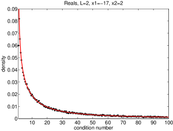
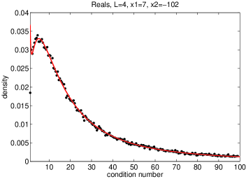
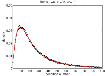
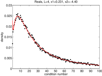
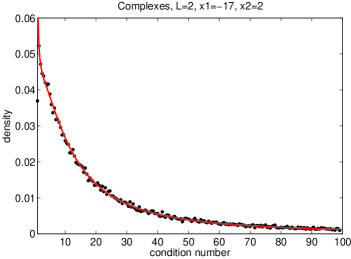
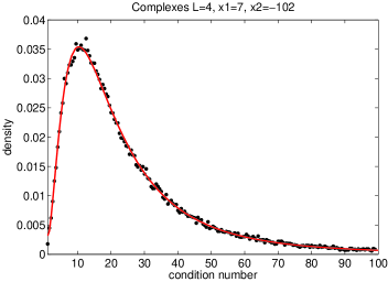
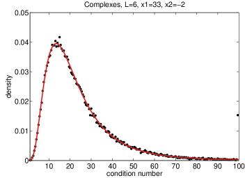
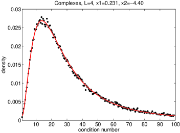
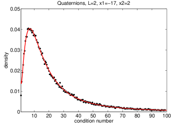
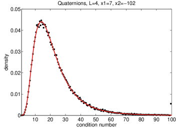
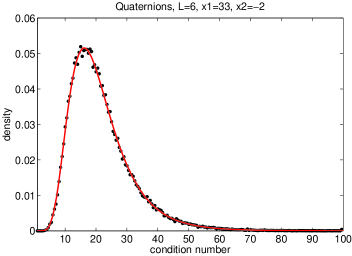
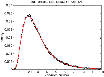
In this section we compare the theoretical condition number distribution, Eq. (Distribution of the Condition Number), (red curves) against Monte Carlo data (black dots) for the three special cases of real, complex and quaternionic matrices $W$. In all the plots the number of trials used to generate Monte Carlo data was $10^{5}$.

Real Matrices $\beta=1$

Figure 1: Real $W$ matrices, $\beta=1$, given by Eq. (Distribution of the Condition Number)

Figure 2: Real $W$ matrices, $\beta=1$, given by Eq. (Distribution of the Condition Number)

Complex Matrices $\beta=2$

Figure 3: Complex $W$ matrices, $\beta=2$, given by Eq. (16)

Figure 4: Complex $W$ matrices, $\beta=2$, given by Eq. (16)

Quaternionic Matrices $\beta=4$

Figure 5: Quaternionic $W$ matrices, $\beta=4$, given by Eq. (Distribution of the Condition Number)

Figure 6: Quaternionic $W$ matrices, $\beta=4$, given by Eq. (Distribution of the Condition Number)

General $\beta$

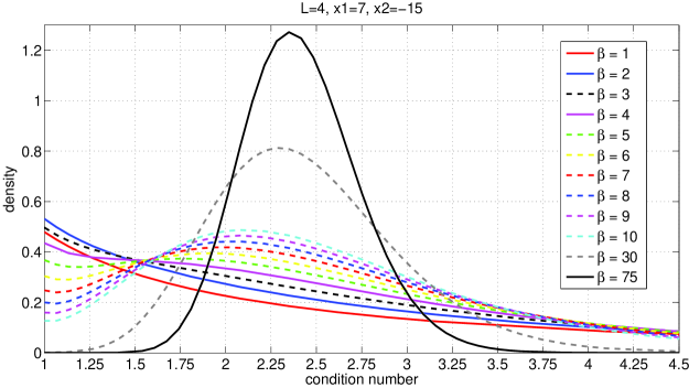
Here we plot Eq. (Distribution of the Condition Number) for a fixed set of parameters $L,x_{1},x_{2}$ for various ghosts.

Figure 7: The condition number density Eq. (Distribution of the Condition Number) for various ghosts. As $\beta\rightarrow\infty$ the distribution becomes non-random and can be represented by a delta function around $2.395$.

Future Work

The natural generalization would be to extend the results to $L\times N$ indefinite matrices. We satisfied ourselves with $N=2$ given its relevance for applications [1, 2].

References

• [1] C. Richmond, R. L. Geddes, R. Movassagh, A. Edelman, “Sample covariance based estimation of Capon algorithm error probabilities”, Signals, Systems and Computers, the Forty Fourth Asilomar Conference (2010)
• [2] C. Richmond, R. L. Geddes, R. Movassagh, A. Edelman, “Performance of sample covariance based capon bearing only tracker”, Signals, Systems and Computers, the Forty Fifth Asilomar Conference (2011)
• [3] L. N. Trefethen, D. Bau III, “Numerical Linear Algebra”, SIAM (1997)
• [4] A. Edelman, Notes for MIT 18.338 “Eigenvalues of Random Matrices”, unpublished.
• [5] R. Muirhead, “Aspects of Multivariate Statistical Theory”, Wiley-Interscience; 2nd edition (2005)
• [6] A. Edelman, “The Random Matrix Technique of Ghosts and Shadows” Markov Processes and Related Fields (2011)
• [7] I.S. Gradshteyn, I.M. Ryzhik, “Table of Integrals, Series and Products”, Academic Press Inc.; 2nd edition (1980)