Current-activity versus local-current fluctuations in driven flow with exclusion

Abstract

We consider fluctuations of steady-state current activity, and of its dynamic counterpart, the local current, for the one-dimensional totally asymmetric simple exclusion process. The cumulants of the integrated activity behave similarly to those of the local current, except that they do not capture the anomalous scaling behavior in the maximal-current phase and at its boundaries. This indicates that the systemwide sampling at equal times, characteristic of the instantaneous activity, overshadows the subtler effects which come about from non-equal time correlations, and are responsible for anomalous scaling. We show that apparently conflicting results concerning asymmetry (skewness) of the corresponding distributions can in fact be reconciled, and that (apart from a few well-understood exceptional cases) for both activity and local current one has positive skew deep within the low-current phase, and negative skew everywhere else.

I Introduction

In this paper we consider fluctuations of the steady-state current, and of its close relative, the current activity, in the one-dimensional totally asymmetric simple exclusion process (TASEP). This model is among the simplest in non-equilibrium physics, while at the same time exhibiting many non-trivial properties derr98 ; sch00 ; derr93 ; rbs01 ; be07 ; cmz11 . Some relevant developments in the study of current fluctuations are as follows: exact expressions for the diffusion constant were found for systems with periodic (PBC) dem93 and open dem95 boundary conditions (BC); the full probability distribution function (PDF) of current fluctuations was similarly considered for both PBC dl98 and open bd06 BC. Very recently, a number of new results have been found for current fluctuations in systems with open BC kvo10 ; gv11 ; lm11 ; ess11 .

In a recent publication rbsdq12 , exact and numerical results were given for steady-state current activity fluctuations in the one-dimensional TASEP, for both periodic and open boundary conditions. By making use of the known steady-state operator algebra derr93 , exact expressions were derived for the three lowest moments of the activity PDF, which fully display their finite-size dependence. All these were confirmed to excellent degree of accuracy by numerical simulations. The results of Ref. rbsdq12, extend and complement earlier analytic work on the joint distribution of current activity and density for the TASEP ds04 ; ds05 . We recall that the current activity (henceforth denominated simply activity) is not identical to the standard current, although the first moments of the respective distributions coincide. As explained below, the former quantity is static, in this sense akin to the instantaneous (local or global) particle density, while the latter is a dynamic one.

Many exact results available for current fluctuations pertain to the infinite-system limit dl98 ; bd06 ; ess11 , although the diffusion constant has been calculated for finite systems dem93 ; dem95 . Finite-size effects have been considered also, e.g., in Refs. kvo10, ; gv11, ; lm11, .

Our main purpose here is to exploit the possible connections between activity- and current fluctuations. Given that the former quantity has proved amenable to such detailed description, it is desirable to check whether its properties can help explain any relevant aspects of the latter.

In the time evolution of the $1+1$ dimensional TASEP, the particle number $n_{\ell}$ at lattice site $\ell$ can be $0$ or $1$, and the forward hopping of particles is only to an empty adjacent site. The stochastic character comes from random selection of site occupation update rsss98 ; dqrbs08 : if site $\ell$ is chosen for update, the instantaneous current across the bond from $\ell$ to $\ell+1$ is given by $J_{\ell,\ell+1}=n_{\ell}(1-n_{\ell+1})$ .

With open boundary conditions, the case considered here, the additional externally-imposed parameters are: the injection (attempt) rate $\alpha$ at the left end, and the ejection rate $\beta$ at the right one. The phase diagram in $\alpha$–$\beta$ parameter space, reproduced in Figure 1 below, is known exactly, as well as many other steady state properties derr98 ; sch00 ; derr93 ; rbs01 ; be07 ; ds04 ; ds05 ; nas02 ; ess05 .

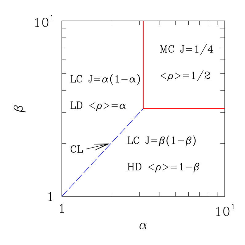
Figure 1: (Color online) Phase diagram of TASEP with open BC. Values of steady-state current $J$ and density $\langle\rho\rangle$ correspond to $L\to\infty$. The low-current (LC), low-density (LD) phase is separated from the LC, high-density (HD) phase by a first-order transition along the coexistence line CL (long-dashed, blue). The maximal-current (MC) phase is separated from the LC phases by second-order transition lines (full red lines).

The total (instantaneous) activity $A$ within the system is defined as the number of bonds that can facilitate a transition of a particle in the immediate future. Thus it equals the number of pairs of neighboring sites that have a particle to the left and a hole to the right ds04 ; ds05 . For systems with open BC, one usually includes also the injection and ejection bonds at the system’s ends, though these have to be weighted by the respective injection and ejection rates, $\alpha$ and $\beta$.

For an $L$–site system with open BC ($L$ sites and $L+1$ bonds, including the injection and ejection ones), one has:

$$A=\alpha\,(1-n_{1})+\sum_{\ell=1}^{L-1}n_{\ell}\,(1-n_{\ell+1})+\beta\,n_{L}\quad{\rm(Open\ BC)}\ .$$ (1)

The activity is a snapshot of the system at a given moment in its evolution; in this sense, it is as much of a static quantity as, for example, the instantaneous global density. By contrast, the current is a dynamic object, as it reflects the stochastically-determined particle displacements which actually take place during a unit time interval. The investigation of current fluctuations is usually carried out by examining the total charge (i.e., number of particles) crossing a given bond, during a long time interval in the steady state regime dem95 ; dl98 ; bd06 ; kvo10 ; gv11 ; lm11 ; ess11 .

The (properly normalized) first moments of activity and current PDFs coincide. For $A$ as defined in Eq. (1) one has:

$$J=\frac{1}{L+1}\,\langle A\rangle\qquad{\rm(Open\ BC)}\ ,$$ (2)

where $J$ is the average steady-state current through any bond in the system, and brackets $\langle\dots\rangle$ denote ensemble averages. The above equality can be understood by recalling that successive steady-state snapshots (activity configurations) are generated via the intervening particle hoppings, which constitute realizations of the system’s current. In our simulations of Ref. rbsdq12, we verified that this property holds, to within numerical accuracy, in all cases investigated there. However, the connection at this level is not sufficient to warrant equality of higher moments of the PDFs.

Here we restrict ourselves to the second and third cumulants of current- and activity PDFs. These already provide significant illustrations of the diversity of behavior which it is our purpose to investigate. While more precise definitions are deferred to Section II below, Tables 1 and 2, and Figure 2, give a broad perspective of properties, such as system-size dependence or $L\to\infty$ limiting values, of these cumulants, or quantities associated to them (respectively, variance and skewness rbsdq12 ; numrec for activity; diffusion constant dem95 and skew lm11 ; ess11 for current). All quoted results for activity statistics were previously published in Ref. rbsdq12, , having been obtained analytically, and supported by numerical simulations; those for current statistics are exact predictions found by assorted analytic techniques dem95 ; lm11 ; ess11 .

Table 1: For systems with $L$ sites, $\alpha$, $\beta$ as specified, and $\gamma\equiv{\rm min}(\alpha,\beta)$, system-size dependence of: (i) variance for (normalized) activity PDF [ see Eq. (2) ], and (ii) diffusion constant dem95 for current (in the latter, values quoted for LC phase correspond to $L\to\infty$).

Variance / Diffusion constant
Region	Activity rbsdq12	Current
LC $[\,\gamma<1/2\,]$	$L^{-1}$	$\gamma(1-\gamma)(1-2\gamma)$ dem95 ; lm11 ; ess11
MC $[\,(\alpha,\beta)>1/2\,$]	$L^{-1}$	$L^{-1/2}$ dem95 ; lm11

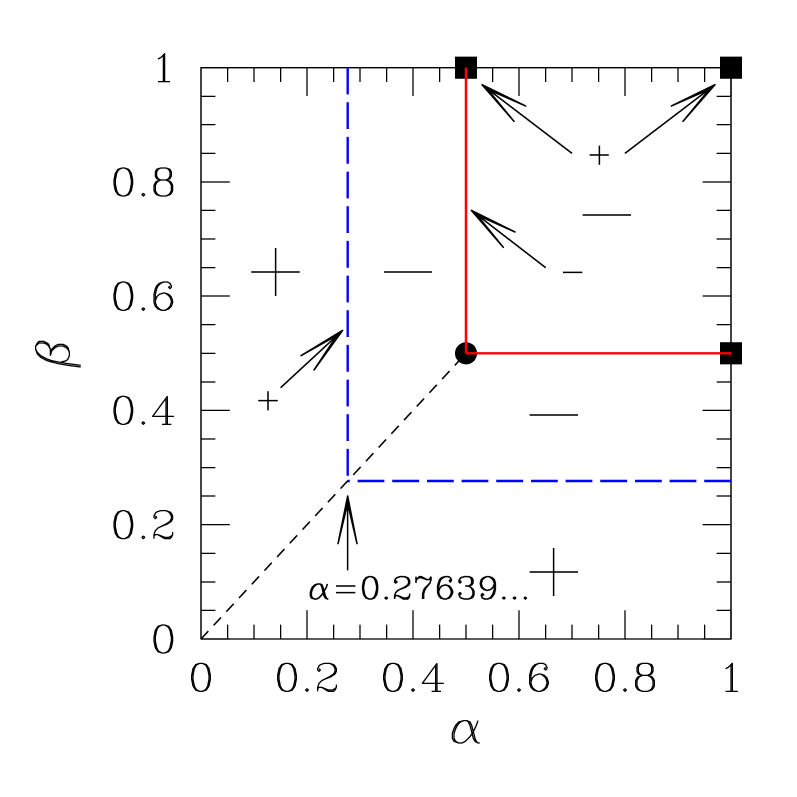
Figure 2: (Color online) The sign of skewness $S$ rbsdq12 ; numrec of the activity PDF in the various regions of the $\alpha-\beta$ phase diagram is shown. The large–$L$ dependence, $|S|\propto L^{-x}$, is $x=1/2$ in the LC phases [${\rm min}\,(\alpha,\beta)<1/2$] except for the long-dashed (blue) lines at ${\rm min}\,(\alpha,\beta)=\frac{1}{2}-\frac{\sqrt{5}}{10}=0.27639\dots$ $[\,x=3/2\,]$. In the MC phase $\alpha,\beta>1/2$, and on the full (red) lines separating MC and LC phases: $x=3/2$. Full squares: $x=5/2$. On the $\alpha=1$ and $\beta=1$ lines, $S$ has the same sign and $L$-dependence as in the respective adjacent regions, except for the points marked by full squares. The circle marks $(\alpha,\beta)=(1/2,1/2)$ where $S\equiv 0$. The short-dashed line is the coexistence line between HD and LD phases. Because of particle-hole duality, $S$ is the same for pairs of points symmetric with respect to the $\alpha=\beta$ line. (Adapted from Figure 8 of Ref. rbsdq12, ).

Table 2: For systems with $\alpha$, $\beta$ as specified, and $\gamma\equiv{\rm min}(\alpha,\beta)$, predicted $L\to\infty$ properties of skew (third cumulant) of current PDF.

Skew
Region/point	Analytic prediction
LC $[\,\gamma<1/2\,]$	$\gamma(1-\gamma)(1-6\gamma+6\gamma^{2})$ lm11 ; ess11
MC $[\,(\alpha,\beta)>1/2\,$]	$<0$ lm11
$(\alpha,\beta)=1$	$-0.009\,0978\,\dots$ lm11

So, all quantities associated with activity statistics vanish as $L\to\infty$ (except for the skewness at $\alpha=\beta=1/2$ which vanishes identically rbsdq12 , see caption to Fig. 2), while those related to the standard current usually approach finite limits (except for the diffusion constant in the MC phase, see Table 1, and the skew on the lines ${\rm min}(\alpha,\beta)\equiv\gamma_{0}=\frac{1}{2}-\frac{\sqrt{5}}{10}$ deep inside the LC phase, see Table 2).

Here we wish to pin down the causes for such variety of behavior in apparently similar fluctuation-related quantities. As shown in the following, a fruitful line of enquiry is to probe the relative importance of different types of correlations which occur in this context: local versus global (i.e. systemwide), as well as equal- versus non-equal time (see Section II for precise definitions).

Section II below recalls selected existing results, and gives a theoretical background to the concepts used in this work. In Section III, our numerical simulations are described, and their corresponding results are exhibited. In Sec. IV we provide a global analysis of the numerical results; finally, concluding remarks are made.

II Theory

In studies of current fluctuations for the TASEP, one considers the steady-state current through a specified bond connecting sites $\ell$ and $\ell+1$, henceforth denoted by $J_{\ell}$, and the associated integrated charge ${\widetilde{Q}}_{\ell}(t)\equiv\int_{0}^{t}J_{\ell}(t^{\prime})\,dt^{\prime}$. With open BC, the leftmost (injection) bond $\ell=0$ is usually singled out for examination, although the results for the PDF of steady-state current fluctuations would be the same for any choice of $\ell$ dem95 . Thus, here we frequently omit bond labels wherever this does not give rise to ambiguity. Also, it is usual to remove the linear term from the integrated charge, and to consider instead:

$$Q(t)\equiv{\widetilde{Q}}(t)-Jt\ ,$$ (3)

so $\langle Q(t)\rangle\equiv 0$. Closed-form expressions are available for $J$ as a function of $\alpha$, $\beta$, and number of sites $L$ derr93 ; see, e.g., Eqs. (29) and (32)–(34) of Ref. rbsdq12, .

For $t\to\infty$, exact expressions for the lowest-order cumulants, $\langle\langle Q^{n}\rangle\rangle$, of the integrated current have been proposed: for $n=2$ and any $L$, everywhere on the phase diagram dem95 ; for $n=1-3$ and $L\to\infty$, anywhere except for the maximal-current phase $\alpha$, $\beta\geq 1/2$ ess11 ; and (via a parametric representation) for any $\alpha$, $\beta$, and $L$, essentially for all $n$ lm11 . In the latter, explicit expressions are forthcoming only for $L\to\infty$ away from the maximal-current phase, and for $n\leq 3$, any $L$, at $(\alpha,\beta)=(1,1)$. The above results agree with each other, wherever comparison is possible. Furthermore, on the basis of general properties of the associated generating function (see e.g. Ref. lm11, ), the assumption is made that all cumulants scale linearly with time, so the quantities of interest are the $E_{n}\equiv\langle\langle Q^{n}\rangle\rangle/t$, which are frequently referred to as cumulants of the local current ess11 . So, $E_{2}$ is the diffusion constant, and $E_{3}$ the skew, both mentioned in connection with Tables 1 and 2.

A direct elementary illustration of such linear dependence can be given by considering the variance $\langle\langle{Q}^{2}(t)\rangle\rangle$ . With $\delta J_{\ell}(t)\equiv J_{\ell}(t)-J$, assuming an exponential decay of the current-current correlation function, $\langle\delta J_{\ell}(t^{\prime})\,\delta J_{\ell}(t^{\prime\prime})\rangle\sim e^{-|t^{\prime}-t^{\prime\prime}|/\tau}$, and using steady-state properties, one has:

$$\langle\langle{Q}^{2}(t)\rangle\rangle=\int_{0}^{t}dt^{\prime}\int_{0}^{t}dt^{\prime\prime}\langle\delta J_{\ell}(t^{\prime})\,\delta J_{\ell}(t^{\prime\prime})\rangle=$$

$$\quad({\rm for}\ t\gg\tau)=t\,\int_{0}^{t}ds\,\langle\delta J_{\ell}(0)\,\delta J_{\ell}(s)\rangle=t\tau\ .$$ (4)

An interesting exception to the above has been pointed out in Ref. kvo10, , where theoretical and numerical arguments are presented to show that $\langle\langle Q^{n}\rangle\rangle\sim t^{\,n/3}$ for $n>1$ at the second-order phase boundary between low- and maximal-current phases. We shall return to this later.

As recalled in Eq. (4), the cumulants $\langle\langle Q^{n}\rangle\rangle$, $n>1$, involve unequal-time correlations dem95 , because the integrated charge accumulates local current fluctuations over time. In contrast, see Eq. (1), the nontrivial features of (instantaneous) activity statistics arise because it adds contributions from all sites in the system, thus it depends on non-local, equal-time, correlations rbsdq12 . In fact, it is because $A(t)$ is the sum of ${\mathcal{O}}(L)$ equal-time stochastic (albeit not independent) variables that the variance and skewness (and, most likely, higher-order moments) of its PDF always approach zero for large $L$ rbsdq12 . The spatially local character of the $\langle\langle Q^{n}\rangle\rangle$, in turn, implies less severe $L$-dependent effects on these quantities; thus the $E_{n}$ generally converge towards non-zero values for $L\to\infty$ dem95 ; ess11 ; lm11 .

As stated in Section I, we wish to consider the relative importance of local and non-local (equal and non-equal time) correlations. We then define a hybrid quantity, the position-averaged (instantaneous) current ${\mathcal{J}}(t)$:

$${\mathcal{J}}(t)=\frac{1}{L+1}\sum_{\ell=0}^{L}J_{\ell}(t)\ .$$ (5)

The ensemble average of ${\mathcal{J}}(t)$ coincides with that of the normalized activity, see Eqs. (1) and (2), and of course with the steady-state current $J$. The cumulants of its integral over time, ${\mathscr{Q}}(t)\equiv\int_{0}^{t}{\mathcal{J}}(t^{\prime})\,dt^{\prime}$ incorporate both equal- and unequal-time (as well as local and non-local) correlations. For consistency, see Eq. (3), we also subtract the linear contribution, $Jt$, from ${\mathscr{Q}}(t)$.

In order to draw relevant distinctions and similarities with ${\mathscr{Q}}(t)$, we also consider the integrated (normalized) activity, ${\mathcal{A}}(t)\equiv(L+1)^{-1}\,\int_{0}^{t}A(t^{\prime})\,dt^{\prime}$ (again, with the linear contribution $Jt$ subtracted).

In what follows, we show results of numerical simulations of ${\mathcal{J}}(t)$ and associated quantities such as the cumulants of ${\mathscr{Q}}(t)$, as well as those of ${\mathcal{A}}(t)$, in comparison with those corresponding to the local current.

III Numerical results

III.1 Introduction

To make contact with previous work, we usually considered lattices either with $L=600$ sites, as done in local-current simulations kvo10 , or with $L=256$, for which many results on activity statistics are available rbsdq12 . It is important to take $L\gg 1$ not only in order to minimize finite-size effects, but also because some features such as the non-linear scaling of current cumulants with time, referred to above, occur only during time "windows" whose width increases as $L$ grows large kvo10 .

In our simulations, a time step is defined as a set of $L$ sequential update attempts, each of these according to the following rules: (1) select a site at random; (2a) if the chosen site is the rightmost one and is occupied, then (3a) eject the particle from it with probability $\beta$; alternatively, (2b) if the site is the leftmost one and is empty, then (3b) inject a particle onto it with probability $\alpha$; finally, if neither (2a) nor (2b) is true, (2c) if the site is occupied and its neighbor to the right is empty, then (3c) move the particle.

Thus, in the course of one time step, some sites may be selected more than once for examination, and some may not be examined at all. This corresponds to the random-sequential update procedure of Ref. rsss98, . Note that other types of update are possible (e.g., ordered-sequential or parallel). Though the resulting phase diagrams are similar in all cases (but not identical: even the average current differs in either case, see Table 1 in Ref. rsss98, ), the updating algorithm which corresponds to the operator algebra described in Ref. derr93, [ and thus to many subsequent results either directly derived from that algebra rbsdq12 , or from Bethe-ansatz techniques which are based on it ess11  ] is random-sequential rsss98 .

For the various sets of $\alpha$, $\beta$ considered here [ because of particle-hole duality, we take only $\alpha\leq\beta\,$], we found that for $L=600$ and starting from an initial random configuration of occupied sites, one needs $n_{\rm in}=10,000$ time steps for steady-state flow to be fully established, so that the $\langle\langle Q^{n}\rangle\rangle$ are free from startup effects (for $\alpha=\beta=1$ this remark needs to be qualified, see Section III.3). Hence we discarded the first $n_{\rm in}$ configurations when evaluating all quantities discussed in the following. As seen below in Figures 3, 4, and 8, the characteristic decay times for the $\langle\langle{\mathscr{Q}}^{n}\rangle\rangle$, $\langle\langle{\mathcal{A}}^{n}\rangle\rangle$ are about twice that, so the respective curves still show some crossover towards pure power-law behavior for the first $\sim 10^{4}$ time steps depicted.

III.2 $\alpha+\beta=1$

It is known derr93 that, for $\alpha+\beta=1$ the correlations between the operators representing particle and vacancy vanish, and they can be represented by $c$-numbers. One consequence of this is that the average current does not exhibit finite-size effects: $J=\alpha\beta$ for any system size. Further simplifications occur, so that simple expressions can also be found for higher-order moments of the activity distribution rbsdq12 [ which is not generally true for points elsewhere on the phase diagram, with the notable exception of $(\alpha,\beta)=(1,1)$ deep inside the MC phase, see Section III.3 ]. Along $\alpha+\beta=1$ we take one point, $(0.3,0.7)$, representative of behavior deep inside the LC phase, and another, $(0.5,0.5)$ on the second-order transition line between LC and MC phases.

In Figure 3 we present the evolution of $\langle\langle{\mathcal{A}}^{2}\rangle\rangle$ and $\langle\langle{\mathscr{Q}}^{2}\rangle\rangle$ against time, for $(\alpha,\beta)=(0.3,0.7)$ and $(0.5,0.5)$. In both cases the variance initially increases faster than linearly with time, but eventually settles to a linear increase. Also, both quantities behave identically for $\alpha=0.3$, $\beta=0.7$, while for the special case $\alpha=\beta=0.5$ they follow very close trends, the ratio $\langle\langle{\mathcal{A}}^{2}\rangle\rangle/\langle\langle{\mathscr{Q}}^{2}\rangle\rangle$ starting at around $0.85$ and approaching unity as $t$ grows (near the upper limit in the Figure, it has reached $0.95$).

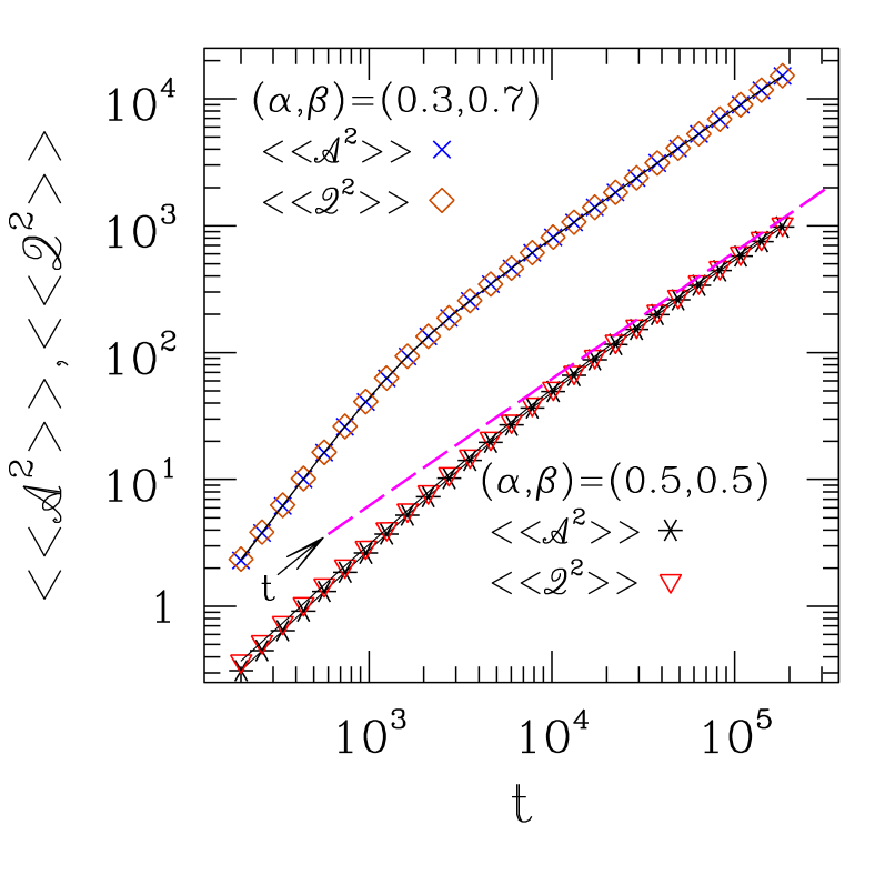
Figure 3: (Color online) Double-logarithmic plot of variances $\langle\langle{\mathcal{A}}^{2}\rangle\rangle$, for the integrated activity ${\mathcal{A}}(t)$, and $\langle\langle{\mathscr{Q}}^{\,2}\rangle\rangle$ for ${\mathscr{Q}}(t)$, both defined below Eq. (5), against time. The dashed line is $\propto t$. System size $L=600$.

One sees that the dominant features of the second-order cumulants of $\mathscr{Q}$ essentially coincide with those of $\mathcal{A}$. As shown below, the quantitative description of $n=3$ cumulants, and of their associate skewness properties, always points to their absolute value being rather small; at the level of accuracy pursued here the main issue therefore concerns their sign, which generally proves to be a robust feature (i.e., independent of whether $\mathscr{Q}$ or $\mathcal{A}$ is the quantity under consideration). Thus, in the following, we usually display only results for the $\langle\langle{\mathscr{Q}}^{\,n}\rangle\rangle$, for comparison with the conventional $\langle\langle Q^{\,n}\rangle\rangle$ .

In Figure 4 we show the cumulants $\langle\langle{Q}^{2}\rangle\rangle$ and $\langle\langle{\mathscr{Q}}^{\,2}\rangle\rangle$ against $t$, for $\alpha=0.3$, $\beta=0.7$, and for $\alpha=\beta=0.5$ .

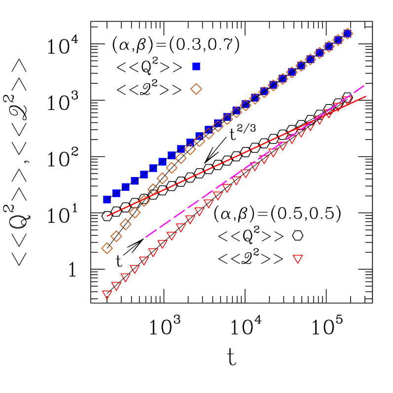
Figure 4: (Color online) Double-logarithmic plot of variances $\langle\langle{Q}^{2}\rangle\rangle$, for $Q(t)$ defined in Eq. (3), and $\langle\langle{\mathscr{Q}}^{\,2}\rangle\rangle$ for ${\mathscr{Q}}(t)$ defined below Eq. (5), against time. The full line is $\propto t^{2/3}$; the dashed line is $\propto t$. System size $L=600$.

Regarding data for $\langle\langle{Q}^{2}\rangle\rangle$ in Fig. 4, for $\alpha=0.3$, $\beta=0.7$ the expected linear behavior against $t$ is present for the whole time interval shown. On the other hand, for $\alpha=\beta=0.5$ one sees the anomalous scaling with $t^{\,2/3}$, referred to above, over a wide time window up to $t\approx 3\times 10^{4}$. Both types of power-law behavior have been reported in Ref. kvo10, , for the same two sets of values of $(\alpha,\beta)$. For the $\alpha=\beta=0.5$ data, at longer times there is a crossover back towards linear scaling.

Anomalous scaling at $\alpha=\beta=0.5$ has been explained in detail in Ref. kvo10, . It can be understood by recalling that this point is on the second-order phase boundary separating low- and maximal-current phases (see Figure 1). The associated diverging correlation length $\xi$ brings about a diverging relaxation time $\tau\sim\xi^{z}$ (where $z=3/2$ is the Kardar-Parisi-Zhang exponent known to describe TASEP dynamics derr98 ; sch00 ; rbs01 ) which, in turn, governs the current-current correlation fluctuations and related quantities. For systems of finite size $L$, this regime holds only for $t\lesssim L^{z}$, i.e., the "windows" referred to earlier. In connection with Eq. (4), it can be seen that in this case, the assumption of $t\gg\tau$ fails over the window of anomalous scaling, but is then restored at longer times; hence, the observed crossover towards linear behavior.

Going now to data for $\langle\langle{\mathscr{Q}}^{2}\rangle\rangle$, one sees that they eventually merge with the respective $\langle\langle{Q}^{2}\rangle\rangle$ curves. For $\alpha=\beta=0.5$ such merging happens, of course, at later times than the window of anomalous scaling. It was shown in Ref. rbsdq12, that the activity PDF is a pure Gaussian at this point; here, as already remarked in connection with Figure 3, we see that $\langle\langle{\mathscr{Q}}^{2}\rangle\rangle$ does not capture the anomalous scaling behavior there, either.

Further information can be extracted from the PDFs, or full counting statistics, of the integrated currents. Data for ${\mathscr{Q}}(t)$ at $(\alpha,\beta)=0.5$ are shown in Figure 5 as a scaling plot. Although the effective scaling power is $1/2$, which is in line with the linear dependence of $\langle\langle{\mathscr{Q}}^{2}\rangle\rangle$ against $t$ seen in Fig. 4, the scaled PDF shows a slight negative skew. For comparison, Figure 6 shows the corresponding scaling plot for $Q(t)$ within the anomalous scaling window, where a negative skew is more clearly present; however, the scaling power is now $1/3$, as already remarked in Ref. kvo10, .

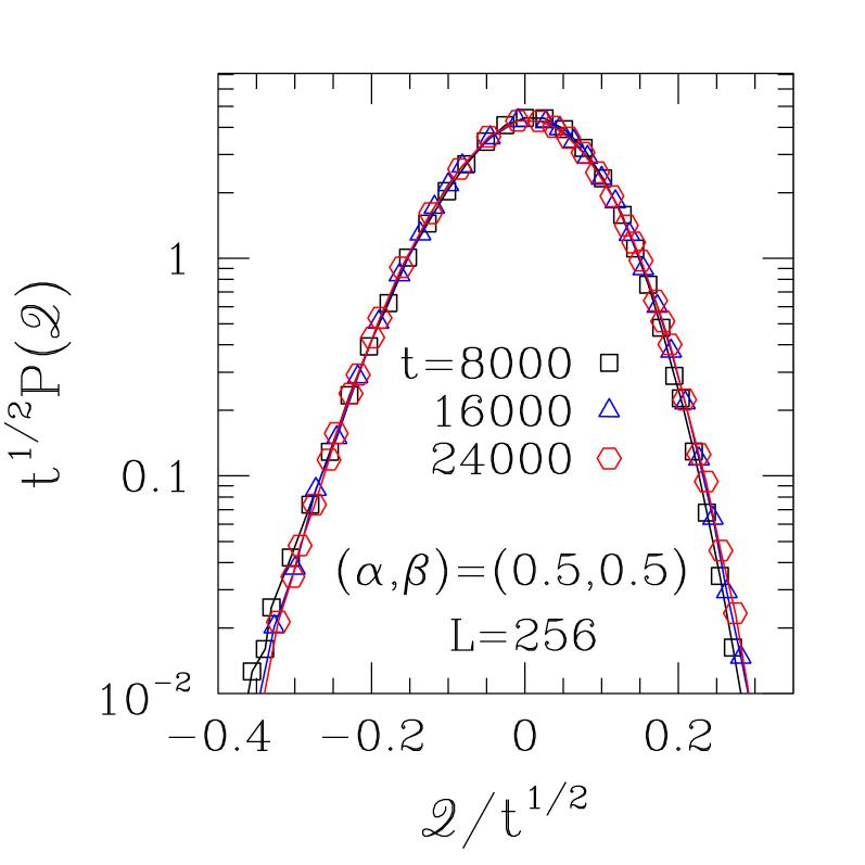
Figure 5: (Color online) Scaling plot of PDF for the variable ${\mathscr{Q}}(t)$ defined below Eq. (5), at $(\alpha,\beta)=(0.5,0.5)$. $N_{\rm sam}=10^{6}$ steady-state samples were collected at the indicated times.

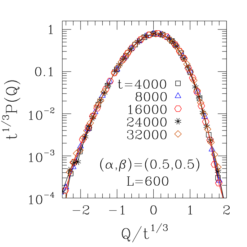
Figure 6: (Color online) Scaling plot of PDF for the variable $Q(t)$ defined in Eq. (3), at $(\alpha,\beta)=(0.5,0.5)$. $N_{\rm sam}=10^{6}$ steady-state samples were collected at the indicated times.

For a proper analysis of the scaled data shown in Figures 5 and 6, and comparison with theoretical predictions where available, one must keep in mind that the former necessarily pertain to finite $t$ and $L$, while the latter either assume taking the $L,t\to\infty$ limit ess11 ; lm11 , or dem95 $L$ is kept fixed and $t\to\infty$.

Denoting by $k$ the scaling powers referred to, it turns out from the scaled variables $u\equiv{\mathscr{Q}}/t^{k}$ [$\,Q/t^{k}\,$] and $P(u)\equiv t^{k}\,P({\mathscr{Q}})$ [$\,t^{k}\,P(Q)\,$] that the cumulants of the global [ local ] current are given by ${\mathcal{E}}_{n}\ [\,E_{n}\,]=t^{nk-1}\,\langle\langle u^{n}\rangle\rangle$ .

So, for the global current ($k=1/2$), one can have both $\langle\langle u^{2}\rangle\rangle$ and ${\mathcal{E}}_{2}$ finite for $t\to\infty$, while $\langle\langle u^{3}\rangle\rangle$ must vanish in the same limit, since ${\mathcal{E}}_{3}$ must not diverge. By separately analyzing PDF data used in Figure 5 for various times $4000\leq t\leq 24000$ we found that, as $t$ increases, ${\mathcal{E}}_{2}=\langle\langle u^{2}\rangle\rangle$ increases from $0.0077$ to $0.0081$, while $\langle\langle u^{3}\rangle\rangle$ goes from $-2.7\times 10^{-4}$ to $-1.4\times 10^{-4}$. The "diffusion constant" ${\mathcal{E}}_{2}$ can be compared with $E_{2}\approx(16\pi L)^{-1/2}=0.0088\dots$ for $L=256$ dem95 . Although there appears to be no a priori reason to assume equality of these quantities, the closeness of their values is remarkable. As regards $\langle\langle u^{3}\rangle\rangle$, its evolution can be approximately matched by a $t^{-1/2}$ dependence, which would be compatible with a nonzero limiting value for ${\mathcal{E}}_{3}$.

For the local current ($k=1/3$), if $\langle\langle u^{2}\rangle\rangle\neq 0$ then $E_{2}=\langle\langle Q^{2}\rangle\rangle/t\sim t^{-1/3}$ which is in line with existing results dem95 ; ess11 ; lm11 , recalling that at $(\alpha,\beta)=(0.5,0.5)$: (i) $E_{2}(L)\propto L^{-1/2}$ dem95 , and (ii) the appropriate finite-size scaling combination is $t/L^{3/2}$. Also, $E_{3}$ should approach a finite value if $\langle\langle u^{3}\rangle\rangle$ is finite. From the full set of data in Figure 5, we find $\langle\langle u^{3}\rangle\rangle=-0.034(1)$ . Separate analysis of subsets of data for different times shows small fluctuations around the average just quoted, with no apparent up- or downward trend upon increasing $t$. Comparison of this estimate to the analytic prediction for the thermodynamic limit, $E_{3}=-1/8$ ess11 ; lm11 shows that, though correct in sign, it is still only about $1/4$ of the expected value.

At $(\alpha,\beta)=(0.3,0.7)$, as evinced in Figure 4, the scaling power is $k=1/2$ for both $\mathscr{Q}$ and $Q$. Figure 7 shows that the scaled PDFs for both quantities are nearly indistinguishable, even when one plots $L=256$ data for $P({\mathscr{Q}})$ together with $L=600$ data for $P(Q)$. Thus, for this range of $L$, deep inside the LC phase the statistics of $Q$ and $\mathscr{Q}$ are essentially identical, and free from finite-size effects. From fits of pure Gaussians to the scaled PDFs, we get ${\mathcal{E}}_{2}\approx E_{2}=0.0841(5)$, in very good agreement with the thermodynamic-limit prediction dem95 ; ess11 ; lm11 $E_{2}=\alpha(1-\alpha)(1-2\alpha)=0.084$. Allowing for non-zero skewness gives $E_{2}\approx 0.082$, with $E_{3}<0$, and $|E_{3}|\lesssim 1\times 10^{-3}$. However, the estimates for the latter quantity exhibit uncertainties of order $60\%$ or thereabouts, so they should be considered with caution. The theoretical prediction for $L\to\infty$ ess11 ; lm11 is $E_{3}=\alpha(1-\alpha)(1-6\alpha+6\alpha^{2})=-0.0546$ . As in the case of ($\alpha,\beta)=(0.5,0.5)$, we get the right sign for $E_{3}$ but a smaller absolute value than predicted.

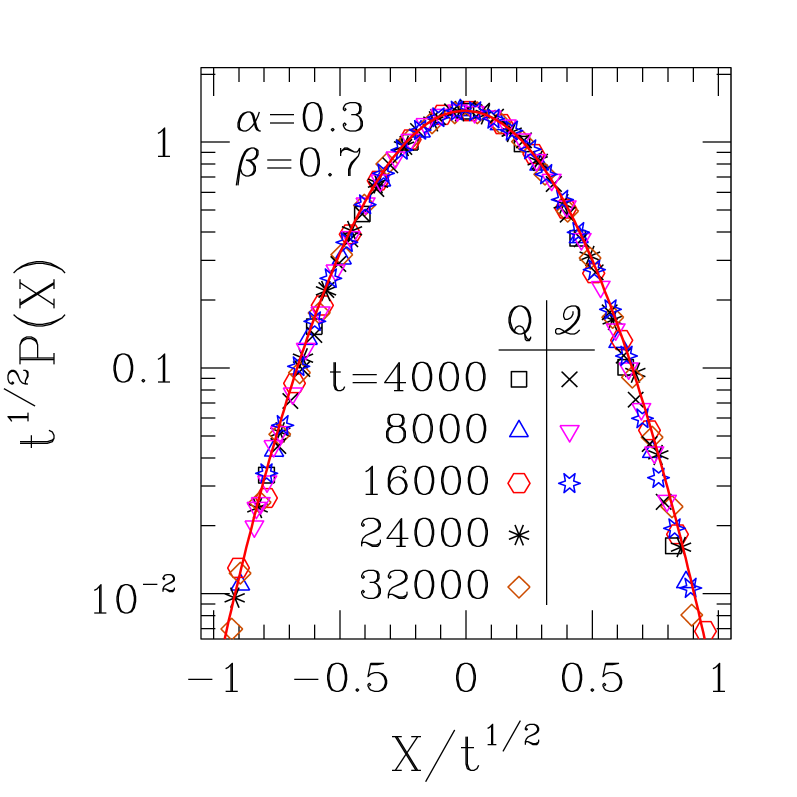
Figure 7: (Color online) Scaling plot of PDFs for: (i) the variable $X=Q(t)$ defined in Eq. (3) [  system size $L=600\,$], and (ii) $X={\mathscr{Q}}(t)$, defined below Eq. (5) [$\,L=256\,$], at $(\alpha,\beta)=(0.3,0.7)$. The full (red) line is a Gaussian fit to data. $N_{\rm sam}=5\times 10^{5}$ steady-state samples were collected at the indicated times .

III.3 $\alpha=\beta=1$

Within the maximal current phase $\alpha,\beta\geq 1/2$, the behavior is expected to be similar to that observed at $(\alpha,\beta)=(0.5,0.5)$, and reported in Section III.2. At $\alpha=\beta=1$ several simplifications occur derr93 ; dem95 ; lm11 ; rbsdq12 , allowing for simple expressions to be derived for the $\langle\langle Q^{n}\rangle\rangle$, so we ran simulations at that point.

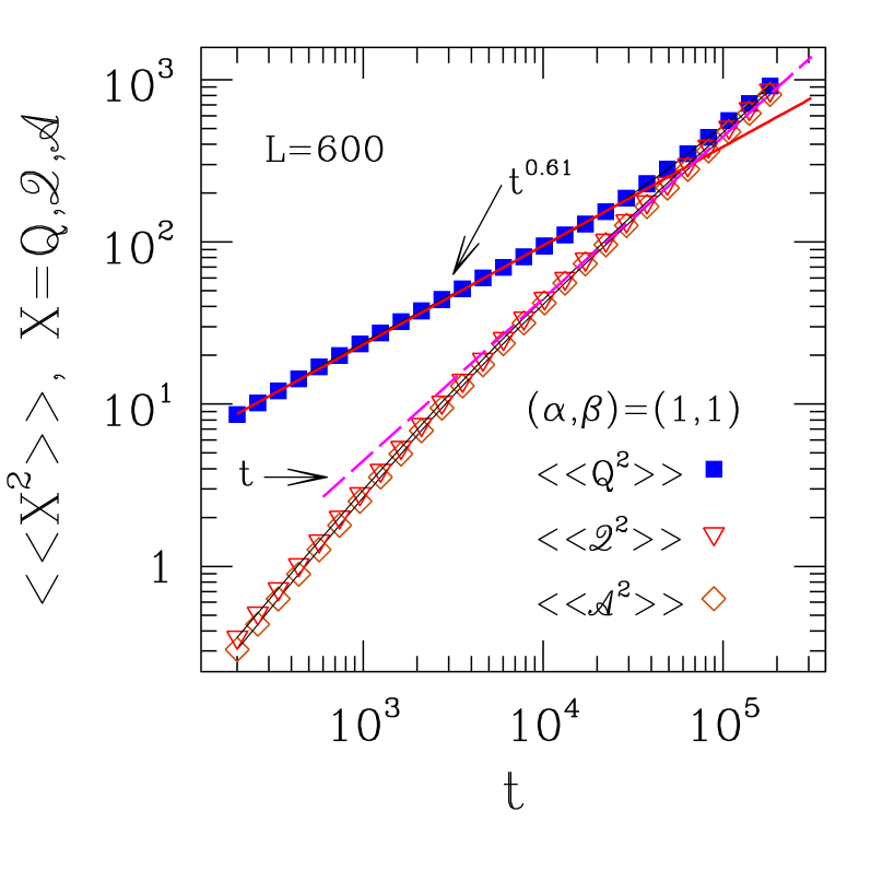
Figure 8: (Color online) At $\alpha=\beta=1$: double-logarithmic plot of variances $\langle\langle{Q}^{2}\rangle\rangle$, for $Q(t)$ defined in Eq. (3), $\langle\langle{\mathscr{Q}}^{\,2}\rangle\rangle$ for ${\mathscr{Q}}(t)$, and $\langle\langle{\mathcal{A}}^{\,2}\rangle\rangle$ for the integrated activity ${\mathcal{A}}(t)$, the latter two defined below Eq. (5), against time. The full line is $\propto t^{0.61}$; the dashed line is $\propto t$.

Figure 8 shows the time evolution of the variance of the several integrated quantities under investigation here. Comparing with Figures 3 and 4, which refer to the same system size and time interval, the main difference to the behavior exhibited at $(\alpha,\beta)=(0.5,0.5)$ is in the anomalous scaling of $\langle\langle Q^{\,2}\rangle\rangle$. Our best fit to single-power behavior, encompassing the same time "window" as used in that case, i.e., $200<t<3\times 10^{4}$, gives an exponent equal to $0.61(1)$, close to but slightly below the expected value, $2/3$. The expected crossover to linear behavior, and merging with the $\langle\langle{\mathscr{Q}}^{\,2}\rangle\rangle$ curve, takes place in the same (narrow) time interval as at $(\alpha,\beta)=(0.5,0.5)$.

The apparent discrepancy in the exponent value can be solved by examining the scaling plot of the PDF for $Q$, shown in Figure 9, where the scaling power is set to $1/3$. It can be seen that data collapse is rather good, except for the $t=4000$ data which visibly stray off, especially at the low end of the curve. Indeed, fitting only data for $8\times 10^{3}<t<3\times 10^{4}$ in Figure 8 gives an exponent $0.66(2)$. So it is the extent of the $t^{\,2/3}$ scaling window which is shorter here than for $(\alpha,\beta)=(0.5,0.5)$ .

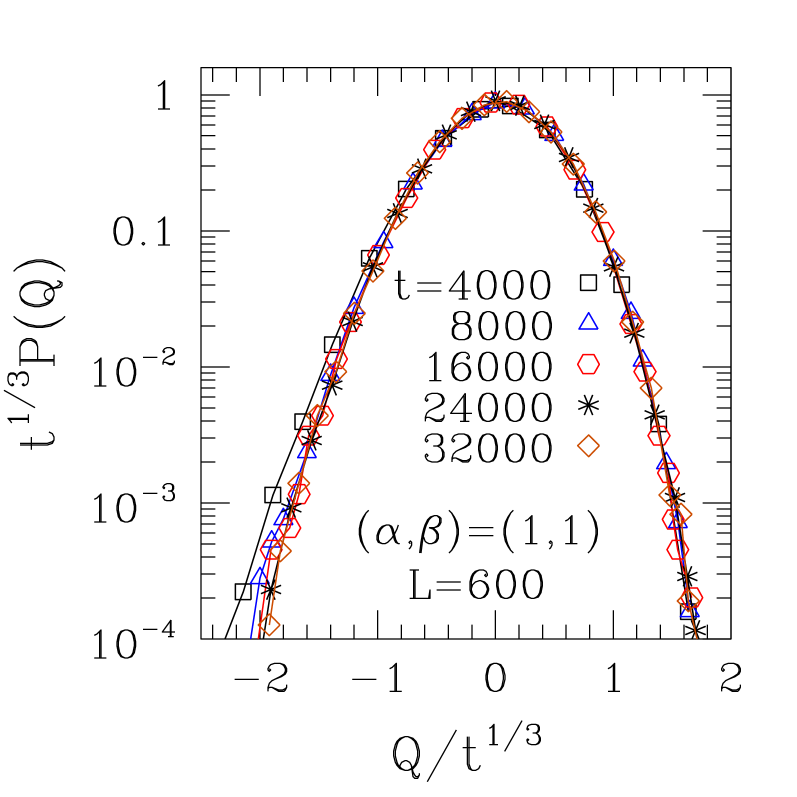
Figure 9: (Color online) Scaling plot of PDF for the variable $Q(t)$ defined in Eq. (3), at $(\alpha,\beta)=(1,1)$. $N_{\rm sam}=5\times 10^{5}$ steady-state samples were collected at the indicated times.

Further analysis of the scaling plot depicted in Figure 9 follows the same lines as that of Figure 6: (i) again, $E_{2}(t)\sim t^{-1/3}$, with the same interpretation as above; and (ii) the value of $\langle\langle u^{3}\rangle\rangle=-0.012(1)$ compares reasonably well to the analytic prediction, $\lim_{L\to\infty}E_{3}=-0.009\dots$ lm11 .

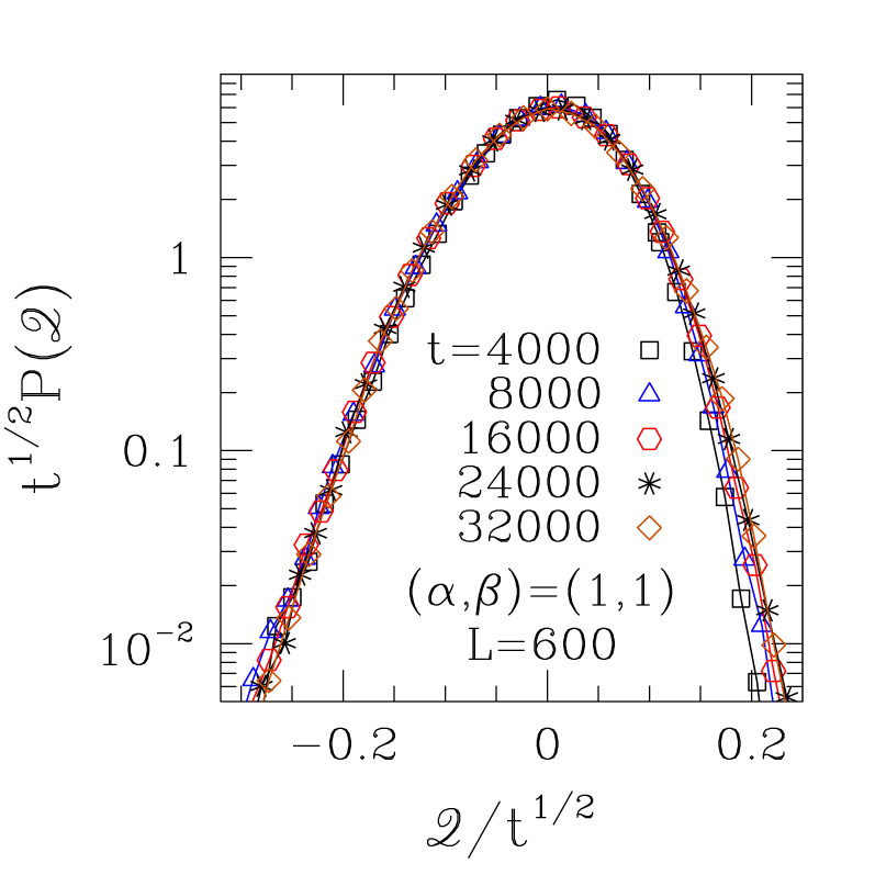
Figure 10: (Color online) Scaling plot of PDF for the variable ${\mathscr{Q}}(t)$ defined below Eq. (5), at $(\alpha,\beta)=(1,1)$. $N_{\rm sam}=10^{6}$ steady-state samples were collected at the indicated times.

Figure 10 shows the scaling plot for the PDF of $\mathscr{Q}$, using $1/2$ as the scaling power. The quality of data collapse is not as good as for points at the border, or outside, of the maximal-current phase (see, respectively, Figures 5 and 7). However, it is possible to find a rather stable estimate for the "diffusion constant", ${\mathcal{E}}_{2}=0.0045(1)$. Again, this compares favorably with $E_{2}=(3\sqrt{2\pi}/64)\,L^{-1/2}=0.004797\dots$ for $L=600$ lm11 . The third cumulant is negative but very close to zero, ${\mathcal{E}}_{3}\approx-1\times 10^{-4}$.

IV Discussion and Conclusions

We have set out to compare the features exhibited by fluctuations of activity with those of (local) current for the TASEP with open BCs.

We define $C_{n}\equiv\langle\langle A^{n}\rangle\rangle$, with the systemwide (instantaneous) activity $A$ defined in Eq. 1, for compatibility with the notation of Ref. rbsdq12, . So ${\mathcal{C}}_{n}\equiv C_{n}/(L+1)^{n}$ is its normalized counterpart. As shown in Ref. rbsdq12, , ${\mathcal{C}}_{2}$ vanishes with system size as $L^{-1}$ for any $(\alpha,\beta)$ (see Table 1). The standard skewness $S$, defined as $S=C_{3}/C_{2}^{3/2}={\mathcal{C}}_{3}/{\mathcal{C}}_{2}^{3/2}$ numrec , vanishes as $L^{-x}$ (so ${\mathcal{C}}_{3}\sim L^{-(x+3/2)}$), usually with $x=1/2$ ($x=3/2$) in the low (high)-current phase, except for some special lines or points on the phase diagram (see Figure 2). As remarked in Section II, ${\mathcal{C}}_{2}$ and ${\mathcal{C}}_{3}$ vanish with increasing $L$ because they reflect fluctuations of the equal-time, nonlocal correlations of ${\mathcal{O}}(L)$ stochastic variables.

On the other hand, cumulants of the integrated activity ${\mathcal{A}}$, as well as those of the position-averaged current ${\mathcal{J}}$, behave similarly (albeit with different decay times on the approach to steady state, see Figures 4 and 8) to those of the local current, except that they do not capture the anomalous scaling which occurs for $\alpha,\beta\geq 1/2$. This indicates that the systemwide sampling at equal times overshadows the subtler effects which come about from non-equal time correlations, within the maximal-current phase and along its border. Anomalous scaling can be unveiled only when the local current is considered, in which case systemwide, equal-time sampling is absent, and the system-size dependence is much less relevant overall (although it still shows up in the width of the scaling "window", see Ref. kvo10, and Figures 4 and 8 above).

Going back to the skewness of distributions, the sign of $S$ is positive for ${\rm min}\,(\alpha,\beta)\leq\frac{1}{2}-\frac{\sqrt{5}}{10}=0.27639\dots$, and negative otherwise, with the following exceptions: $(\alpha,\beta)=(0.5,0.5)$ where $S\equiv 0$, and $(\alpha,\beta)=(1,1)$, $(1,0.5)$, and $(0.5,1)$ where $S>0$ rbsdq12 . At ${\rm min}\,(\alpha,\beta)=0.27639\dots$, $S>0$ but depends on $L^{-3/2}$, as opposed to the $L^{-1/2}$ form which holds generally in the low-current phase. All such exceptions are accidental, i.e., they occur because of symmetries or cancellations which are valid only for those specific values of $(\alpha,\beta)$ rbsdq12 . Furthermore, it has been shown that $S>0$ is to be expected on physical grounds for $\alpha\ll 0.5$ in the low-current, low-density phase (see Figure 3 of Ref. rbsdq12, and accompanying remarks).

Concerning local-current statistics, we recall the results given in Table 2: for the low-current phase Refs. ess11, ; lm11, predict that, with $\gamma\equiv{\rm min}\,(\alpha,\beta)$, $E_{3}=\gamma(1-\gamma)(1-6\gamma+6\gamma^{2})$ which is thus zero for $\gamma_{0}=\frac{1}{2}-\frac{\sqrt{3}}{6}=0.2113\dots$ , and positive (negative) for $\gamma<\gamma_{0}$ ($\gamma>\gamma_{0}$). Ref. lm11, evaluates $E_{3}<0$ at $(\alpha,\beta)=(1,1)$, as recalled in Section III.3, and gives arguments showing that the dominant behavior of the cumulants should be the same as that at $(\alpha,\beta)=(1,1)$ everywhere within the maximal-current phase.

In conclusion, once accidental exceptions are understood as such, both $S$ for activity and $E_{3}$ for the local current tell essentially the same story: fluctuation distributions have positive skew for low injection (or ejection) rates, and negative skew otherwise. The borderline between the two types of behavior lies deep within the low-current phase, and its relationship to the actual (second-order) transition to the maximal-current phase it at best that of a precursor.

As a final remark, we emphasize that accurate numerical checks of the theoretical predictions for $E_{3}$ would need much longer simulations than those reported here, since evaluation of this quantity strongly depends on a proper description of the tails of the local-current PDF. However, at the level of accuracy pursued here, the present results fulfil our goal of providing a comparative analysis of the main features of activity- and local-current fluctuations.

- (1) B. Derrida, Phys. Rep. 301, 65 (1998).
- (2) G. M. Schütz, in Phase Transitions and Critical Phenomena, edited by C. Domb and J. L. Lebowitz (Academic, New York, 2000), Vol. 19.
- (3) B. Derrida, M. Evans, V. Hakim, and V. Pasquier, J. Phys. A 26, 1493 (1993).
- (4) R. B. Stinchcombe, Adv. Phys. 50, 431 (2001).
- (5) R. A. Blythe and M. R. Evans, J. Phys. A 40, R333 (2007).
- (6) T. Chou, K. Mallick, and R. K. P. Zia, Rep. Prog. Phys. 74, 116601 (2011).
- (7) B. Derrida, M. R. Evans, and D. Mukamel, J. Phys. A 26, 4911 (1993).
- (8) B. Derrida, M. R. Evans, and K. Mallick, J. Stat. Phys. 79, 833 (1995).
- (9) B. Derrida and J. L. Lebowitz, Phys. Rev. Lett. 80, 209 (1998).
- (10) T. Bodineau and B. Derrida, J. Stat. Phys. 123, 277 (2006).
- (11) T. Karzig and F. von Oppen, Phys. Rev. B81, 045317 (2010).
- (12) M. Gorissen and C. Vanderzande, J. Phys. A 44, 115005 (2011).
- (13) A. Lazarescu and K. Mallick, J. Phys. A 44, 315001 (2011).
- (14) J. de Gier and F. H. L. Essler, Phys. Rev. Lett. 107, 010602 (2011).
- (15) R. B. Stinchcombe and S. L. A. de Queiroz, Phys. Rev. E85, 041111 (2012).
- (16) M. Depken and R. Stinchcombe, Phys. Rev. Lett. 93, 040602 (2004).
- (17) M. Depken and R. Stinchcombe, Phys. Rev. E71, 036120 (2005).
- (18) N. Rajewsky, L. Santen, A. Schadschneider, and M. Schreckenberg, J. Stat. Phys. 92, 151 (1998).
- (19) S. L. A. de Queiroz and R. B. Stinchcombe, Phys. Rev. E78, 031106 (2008).
- (20) Z. Nagy, C. Appert, and L. Santen, J. Stat. Phys. 109, 623 (2002).
- (21) J. de Gier and F. H. L. Essler, Phys. Rev. Lett. 95, 240601 (2005); J. Stat. Mech.: Theory Exp. (2006) P12011.
- (22) W. Press, B. Flannery, S. Teukolsky, and W. Vetterling, Numerical Recipes in Fortran, The Art of Scientific Computing, 2nd ed. (Cambridge University Press, Cambridge, England, 1992), Chap 14.