Electrical control of the Kondo effect in a helical edge liquid

Abstract

Magnetic impurities affect the transport properties of the helical edge states of quantum spin Hall insulators by causing single-electron backscattering. We study such a system in the presence of a Rashba spin-orbit interaction induced by an external electric field, showing that this can be used to control the Kondo temperature, as well as the correction to the conductance due to the impurity. Surprisingly, for a strongly anisotropic electron-impurity spin exchange, Kondo screening may get obstructed by the presence of a non-collinear spin interaction mediated by the Rashba coupling. This challenges the expectation that the Kondo effect is stable against time-reversal invariant perturbations.

Introduction. The discovery that HgTe quantum wells support a quantum spin Hall (QSH) state Konig has set off an avalanche of studies addressing the properties of this novel phase of matter Review . A key issue has been to determine the conditions for stability of the current-carrying states at the edge of the sample as this is the feature that most directly impacts prospects for future applications in electronics/spintronics. In the simplest picture of a QSH system the edge states are helical, with counter-propagating electrons carrying opposite spins. By time-reversal invariance electron transport then becomes ballistic, provided that the electron-electron (e-e) interaction is sufficiently well-screened so that higher-order scattering processes do not come into play Wu ; Xu .

The picture gets an added twist when including effects from magnetic impurities, contributed by dopant ions or electrons trapped by potential inhomogeneities. Since an edge electron can backscatter from an impurity via spin exchange, time-reversal invariance no longer protects the helical states from mixing. In addition, correlated two-electron Meidan and inelastic single-electron processes Schmidt ; Lezmy must now also be accounted for. As a result, at high temperatures $T$ electron scattering off the impurity leads to a $\ln(T)$ correction of the conductance at low frequencies $\omega$ M , which, however, vanishes in the dc limit $\omega\rightarrow 0$ T . At low $T$, for weak e-e interactions, the quantized edge conductance $G_{0}=e^{2}/h$ is restored as $T\rightarrow 0$ with power laws distinctive of a helical edge liquid. For strong interactions the edge liquid freezes into an insulator at $T=0$, with thermally induced transport via tunneling of fractionalized charge excitations through the impurity M .

A more complete description of edge transport in a QSH system must include also the presence of a Rashba spin-orbit interaction. This interaction, which can be tuned by an external gate voltage, is a built-in feature of a quantum well WinklerBook . In fact, HgTe quantum wells exhibit some of the largest known Rashba couplings of any semiconductor heterostructures Buhmann . As a consequence, spin is no longer conserved, contrary to what is assumed in the minimal model of a QSH system BHZ . However, since the Rashba interaction preserves time-reversal invariance, Kramers’ theorem guarantees that the edge states are still connected via a time-reversal transformation ("Kramers pair") Kane . Provided that the Rashba interaction is spatially uniform and the e-e interaction is not too strong, this ensures the robustness of the helical edge liquid Strom .

What is the physics with both Kondo and Rashba interactions present? In this paper we address this question with a renormalization group (RG) analysis as well as a linear-response and rate-equation approach. Specifically, we predict that the Kondo temperature $T_{K}$ $-$ which sets the scale below which the electrons screen the impurity $-$ can be controlled by varying the strength of the Rashba interaction. Surprisingly, for a strongly anisotropic Kondo exchange, a non-collinear spin interaction mediated by the Rashba coupling becomes relevant (in the sense of RG) and competes with the Kondo screening. This challenges the expectation that the Kondo effect is stable against time-reversal invariant perturbations Meir . Moreover, we show that the impurity contribution to the dc conductance at temperatures $T\!>\!T_{K}$ can be switched on and off by adjusting the Rashba coupling. With the Rashba coupling being tunable by a gate voltage, this suggests a new inroad to control charge transport at the edge of a QSH device.

Model. To model the edge electrons, we introduce the two-spinors $\Psi^{T}=\big{(}\psi_{\uparrow},\psi_{\downarrow}\big{)}$, where $\psi_{\uparrow}\,(\psi_{\downarrow})$ annihilates a right-moving (left-moving) electron with spin-up (spin-down) along the growth direction of the quantum well. Neglecting e-e interactions, the edge Hamiltonian can then be written as

$$H = v_{F}\int\textrm{d}x\ \Psi^{\dagger}(x)\left[-\textrm{i}\sigma^{z}\partial_{x}\right]\Psi(x)+$$

$$+\alpha\int\textrm{d}x\ \Psi^{\dagger}(x)\left[-\textrm{i}\sigma^{y}\partial_{x}\right]\Psi(x)+$$

$$+\Psi^{\dagger}(0)\left[J_{x}\sigma^{x}S^{x}+J_{y}\sigma^{y}S^{y}+J_{z}\sigma^{z}S^{z}\right]\Psi(0),$$

with $v_{F}$ the Fermi velocity parameterizing the linear kinetic energy. The second term encodes the Rashba interaction of strength $\alpha$, with the third term being an antiferromagnetic Kondo interaction between electrons (with Pauli matrices $\sigma^{i},i=x,y,z$) and a spin-1/2 magnetic impurity (with Pauli matrices $S^{i},i=x,y,z$) at $x=0$. The spin-orbit induced magnetic anisotropy for an impurity at a quantum well interface Ujsaghy implies that $J_{x}=J_{y}\neq J_{z}$ Zitko . Unless otherwise stated, we use $\hbar\,=k_{B}\equiv 1$.

The Rashba term in Eq. (Electrical control of the Kondo effect in a helical edge liquid) can be absorbed into the kinetic term by a a spinor rotation $\Psi\rightarrow\Psi^{\prime}=\mathrm{e}^{-\mathrm{i}\sigma^{x}\theta/2}\Psi$ VO . By rotating also the impurity spin, $\boldsymbol{S}\rightarrow\boldsymbol{S}^{\prime}=\mathrm{e}^{-\mathrm{i}S^{x}\theta/2}\boldsymbol{S}\mathrm{e}^{\mathrm{i}S^{x}\theta/2}$, one obtains $H=H_{0}^{\prime}+H_{K}^{\prime}$, with

$$H_{0}^{\prime} = v_{\alpha}\int\textrm{d}x\ \Psi^{\prime\dagger}(x)\left[-\textrm{i}\sigma^{z^{\prime}}\partial_{x}\right]\Psi^{\prime}(x)$$ (2)

$$H_{K}^{\prime} = \Psi^{\prime\dagger}(0)[J_{x}\sigma^{x}S^{x}+J^{\prime}_{y}\sigma^{y^{\prime}}S^{y^{\prime}}+J^{\prime}_{z}\sigma^{z^{\prime}}S^{z^{\prime}}$$ (3)

$$\qquad\ \ \ +J_{E}(\sigma^{y^{\prime}}S^{z^{\prime}}+\sigma^{z^{\prime}}S^{y^{\prime}})]\Psi^{\prime}(0),$$

where $J^{\prime}_{y}=J_{y}\cos^{2}\theta+J_{z}\sin^{2}\theta$, $J^{\prime}_{z}=J_{z}\cos^{2}\theta+J_{y}\sin^{2}\theta$ and $J_{E}=(J_{y}-J_{z})\cos\theta\sin\theta$. The Rashba rotation angle $\theta$ is determined through $\cos\theta=v_{F}/v_{\alpha}$, $\sin\theta=\alpha/v_{\alpha}$ and $v_{\alpha}=\sqrt{v_{F}^{2}+\alpha^{2}}$. Note that the spin in the rotated basis is quantized along the $z^{\prime}$-direction which forms an angle $\theta$ with the $z$-axis. Also note that the Kondo interaction in the new basis not only becomes spin-nonconserving, but also picks up a non-collinear term for $J_{y}\neq J_{z}$.

Including e-e interactions, and assuming a band filling incommensurate with the lattice Review , time-reversal invariance constrains the possible scattering channels in the rotated basis to dispersive $(\sim\!g_{d})$ and forward $(\sim~{}g_{f})$ scattering, in addition to correlated two-particle backscattering $(\sim\!g_{bs})$ Wu ; Xu and inelastic single-particle backscattering $(\sim\!g_{ie})$ Schmidt ; Lezmy ; Budich at the impurity site. Adding the corresponding interaction terms to $H_{0}^{\prime}$ and $H_{K}^{\prime}$ in (2) and (3), and employing standard bosonization G , the full Hamiltonian for the edge liquid can now be expressed as a free boson model, $(v/2)\!\int\textrm{d}x\!\left((\partial_{x}\varphi)^{2}+(\partial_{x}\vartheta)^{2}\right)$, with three local terms added at $x=0$:

$$H_{K}^{\prime}\!\! \!=\! \!\!\frac{A}{\kappa}\!\cos(\sqrt{4\pi K}\varphi)\!+\!\frac{B}{\kappa}\!\sin(\sqrt{4\pi K}\varphi)\!+\!\frac{C}{\sqrt{K}}\partial_{x}\vartheta$$ (4)

$$H_{bs}^{\prime}\! \!=\! \!\frac{g_{bs}}{2(\pi\kappa)^{2}}\cos(\sqrt{16\pi K}\varphi)$$ (5)

$$H_{ie}^{\prime}\! \!=\! \!\frac{g_{ie}}{2\pi^{2}\sqrt{K}}:(\partial_{x}^{2}\vartheta)\cos(\sqrt{4\pi K}\varphi):$$ (6)

Here $\varphi$ is a nonchiral Bose field with $\vartheta$ its dual, $v\partial_{x}\vartheta=\partial_{t}\varphi$ with $v\!=\![(v_{\alpha}\!+\!g_{f}/\pi)^{2}\!-\!(g_{d}/\pi)^{2}]^{1/2}$, $K=[(\pi v_{\alpha}\!+\!g_{f}-g_{d})/(\pi v_{\alpha}\!+\!g_{f}+g_{d})]^{1/2}$ and $\kappa\,\approx v_{F}/D$ is the edge state penetration depth acting as short-distance cutoff with $D$ the band width, and $:...:$ denotes normal ordering. In $H^{\prime}_{K}$ we have defined $A=J_{x}S^{x}/\pi$, $B=(J^{\prime}_{y}S^{y^{\prime}}+J_{E}S^{z^{\prime}})/\pi$ and $C=(J^{\prime}_{z}S^{z^{\prime}}+J_{E}S^{y^{\prime}})/\pi$.

Kondo temperature. The bosonized theory is tailor-made for a perturbative RG analysis, allowing us to determine the temperature scale below which the edge electrons couple strongly to the impurity. We first note that the backscattering term in (5) is that of the well-known boundary-sine Gordon model. For $K\!<\!2/3$ it dominates over the inelastic backscattering in (6), and turns relevant for $K\!<\!1/4$ with a weak to strong-coupling crossover at a temperature $T_{bs}\approx Dg_{bs}^{1/(1-4K)}$ KaneFisher . As a consequence, the enhancement of backscattering as $T\rightarrow 0$ results in a zero-temperature insulating state when $K<1/4$.

Turning to the Rashba-rotated Kondo interaction $H_{K}^{\prime}$ in Eq. (4), we obtain for its one-loop RG equations:

$$\partial_{l}\tilde{J}_{x}=(1\!-\!K)\tilde{J}_{x}+\nu K(\tilde{J}_{y}^{\prime}\tilde{J}_{z}^{\prime}\!-\!\tilde{J}_{E1}\tilde{J}_{E2})$$

$$\partial_{l}\tilde{J}_{y}^{\prime}=(1\!-\!K)\tilde{J}_{y}^{\prime}+\nu K\tilde{J}_{x}\tilde{J}_{z}^{\prime},\ \ \partial_{l}\tilde{J}_{z}^{\prime}=\nu K\tilde{J}_{x}\tilde{J}_{y}^{\prime},$$ (7)

$$\partial_{l}\tilde{J}_{E1}=(1\!-\!K)\tilde{J}_{E1}-\nu K\tilde{J}_{x}\tilde{J}_{E2},\ \ \partial_{l}\tilde{J}_{E2}\!=\!-\nu K\tilde{J}_{x}\tilde{J}_{E1},$$

with the ”tilde” indicating that the couplings depend on the renormalization length $l$, and where $\nu\equiv 1/(\pi v)$. The two terms proportional to $J_{E}$ in Eq. (4) flow individually under RG, with the corresponding renormalized coupling constants here denoted $\tilde{J}_{E1}$ and $\tilde{J}_{E2}$. In deriving Eqs. (7) we have used that higher-order contributions involving an intermediate process governed by $H_{bs}^{\prime}$ or $H_{ie}^{\prime}$ are suppressed, since these transfer spin or energy incompatible with $H_{K}^{\prime}$. In a recent work M2 , Kondo scattering without Rashba interaction was studied, and different physics in the regime $\nu J_{z}\geq 2K$ was found, not accessible perturbatively in $\nu J_{z}$. Since its realization in an HgTe quantum well requires anomalously weak screening of the e-e interaction we do not consider this regime here.

The role of the Rashba rotation in Eqs. (7) is both to determine the bare values $\tilde{J}^{\prime}_{y,z}(l=0)\equiv J^{\prime}_{y,z}$ and to introduce the non-collinear couplings $\tilde{J}_{E1,E2}$. To explore the outcome, we first examine the case of a strongly screened e-e interaction, $K\approx 1$. For this case, the first-order terms of Eq. (7) can be neglected and $\tilde{J}_{E1}=\tilde{J}_{E2}=\tilde{J}_{E}$, since their scaling equations will be identical. In this limit, $\tilde{J}_{E}$ quickly flows to zero. We take the Kondo temperature $T_{K}$ to be the value of $T=D\exp(-l)$ where one of the couplings in Eq. (7) first grows past $1/(\nu K)$, making the renormalized $H_{K}^{\prime}$ in Eq. (4) dominate the free theory. For $K\approx 1$ we then see that

$$T_{K}\approx D\exp\left(-\frac{1}{\nu J_{x}}\frac{\operatorname{arcsinh}(\zeta)}{\zeta}\right),$$ (8)

where $\zeta=\sqrt{(J_{z}/J_{x})^{2}-1}$ is an anisotropy parameter M . Here the $\theta$ dependence lies predominantly in $\nu$. Note that Kondo temperatures modified by spin-orbit couplings, as in (8), or by spin-dependent hopping, have recently been proposed also for ordinary conduction electrons Schuricht ; Feng ; Zitko2 ; Zarea ; Isaev .

In the opposite limit of a strong e-e interaction, the second-order terms of the scaling equations can be neglected, as long as $1-K\gg\tilde{J}\nu K$, for all $\tilde{J}=\tilde{J}_{x},\tilde{J}^{\prime}_{y},\tilde{J}_{E1}$. The scaling equations in this limit reduce to $\partial_{l}\tilde{J}=(1-K)\tilde{J}$, with solutions $\tilde{J}=Je^{(1-K)l}$. With $l=\ln(D/T)$, one can now use the $\tilde{J}=1/(\nu K)$ criterion to find the Kondo temperature

$$T_{K}\approx D\left(J_{max}\,\nu K\right)^{1/(1-K)},$$ (9)

where $J_{max}=\max[J_{x},J^{\prime}_{y},J_{E}]$.

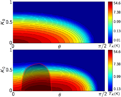
Figure 1: The Kondo temperature $T_{K}$ as a function of the Rashba angle $\theta$ and the ordinary Luttinger parameter $K_{0}$. The $T_{K}$ scale is logarithmic and red and blue color indicates high and low $T_{K}$, respectively. Top: $J_{x}=J_{y}\geq J_{z}$ (here, $J_{x}/a_{0}=J_{z}/a_{0}=10$meV), bottom: $J_{x}=J_{y}<J_{z}$ (here, $J_{x}/a_{0}=5$ meV and $J_{z}/a_{0}=50$ meV). In the shaded area, $\tilde{J}_{E1}$ dominates the perturbative RG flow, hence obstructing singlet formation.

In Fig. (1) we exhibit $T_{K}$ for both ”easy-plane” and ”easy-axis” Kondo interaction. To isolate the effect of the Rashba interaction from that of the e-e interaction we choose to plot $T_{K}$ as a function of $\theta$ and $K_{0}$, with $K_{0}\equiv K(\theta$$=$$0)$ the ordinary Luttinger parameter. For $|J_{E}|>\left|J_{x}\right|,\left|J^{\prime}_{y}\right|$, the non-collinear term $\sim\sigma^{y^{\prime}}S^{z^{\prime}}$ in Eq. (3) dominates the RG flow for values of $K$ in the shaded ”dome” (the size of which is set by the ratio $J_{z}/J_{x,y}$). As this term disfavors a spin singlet, Kondo screening will be obstructed in the corresponding interval of Rashba couplings domefootnote . This runs contrary to the expectation that a spin-orbit interaction does not impair the Kondo effect Meir ; Malecki . However, this expectation is rooted in a noninteracting quasiparticle picture which breaks down in one dimension. Instead a Luttinger liquid is formed, with strongly correlated electron scattering G . As suggested by our RG analysis, when this scattering gets enhanced with lower values of $K$, it boosts the effect of the non-collinear spin interaction that works against the Kondo screening.

Conductance at low temperatures. Away from the ”dome” in Fig. (1), the Rashba-rotated Kondo interaction easily sustains a Kondo temperature $T_{K}$ below which the impurity gets screened. When $K>1/4$ and two-particle backscattering is RG-irrelevant, there is no correction $\delta G$ to the conductance at zero temperature: As explained by Maciejko et al. M , the topological nature of the QSH state implies a "healing" of the edge after the impurity has been effectively removed by the Kondo screening. For finite $T\!\ll\!T_{K}$, the leading correction $\delta G$ is generated by either $H_{bs}^{\prime}$ or $H_{ie}^{\prime}$, whatever operator has the lowest scaling dimension: For $1/4<\!K<\!2/3\,(K>2/3)$ $H_{bs}^{\prime}\,(H_{ie}^{\prime})$ dominates, with $\delta G_{bs}\sim(T/T_{K})^{8K-2}$ M $(\delta G_{ie}\sim(T/T_{K})^{2K+2}$ Schmidt ; Lezmy ). The picture changes dramatically for $K<1/4$. Now $H_{bs}$ turns RG-relevant, with $g_{bs}$ entering a strong-coupling regime below the crossover-temperature $T_{bs}$, implying zero conductance at $T=0$. At finite $T\ll T_{bs}$, instanton processes restore its finite value, with $G\sim(T/T_{bs})^{2(1/4K-1)}$ M . To leading order this regime is blind to the Rashba interaction.

Conductance and currents at high temperatures. When $T>\mbox{max}(T_{K},T_{bs})$, scattering from $H_{K}^{\prime}$ as well as from $H_{bs}^{\prime}$ and $H_{ie}^{\prime}$ remain weak, and transport properties can be obtained perturbatively. We here focus on the correction $\delta G$ to the conductance due to $H_{K}^{\prime}$, noting that the contributions from $H_{bs}^{\prime}$ and $H_{ie}^{\prime}$ decouple and are insensitive to the strength of the Rashba interaction.

The current operator $\hat{I}$ takes the form $\hat{I}=(e/2)\,\partial_{t}\,(\Psi^{\prime\dagger}\sigma^{z^{\prime}}\Psi^{\prime})$ in the rotated basis, since the components of the rotated spinor define new right and left movers. After the unitary transformation $U=\mathrm{e}^{\mathrm{i}\sqrt{\pi}\lambda\varphi(0)S^{z\prime}}$, which removes the $J^{\prime}_{z}$-term when $\lambda=J^{\prime}_{z}/\pi v\sqrt{K}$, the bosonized part $\delta\hat{I}$ of the current operator due to $H_{K}^{\prime}$ is

$$\delta\hat{I} =\frac{\mathrm{i}e}{2\pi\kappa}\big{[}\!\sum_{j=\pm}\!A_{j}e^{\mathrm{i\sqrt{\pi}}(2\sqrt{K}-j\lambda)\varphi}S^{j}+\mathrm{i}A_{0}\,e^{\mathrm{i}\sqrt{4\pi K}\varphi}S^{z}\big{]}$$

$$\hskip 170.71652pt+\mbox{H.c.}$$ (10)

where $A_{\pm}=(1/2)(J_{x}\pm J^{\prime}_{y})$, and $A_{0}=J_{E}/2$. Using the Kubo formula to calculate the conductance correction $\delta G(\omega)$ at a frequency $\omega$ in the limit $J^{2}\ll\omega\ll T$, with $J^{2}=J_{x}^{2},J_{y}^{\prime 2},J_{E}^{2}$, we then find to $\mathcal{O}(J^{2})$

$$\delta G=-\,\frac{e^{2}}{\hbar}\sum_{j=-1}^{+1}A_{j}^{2}\cdot F(2\sqrt{K}-j\lambda)\cdot(2\pi T/D)^{2(\sqrt{K}-j\lambda/2)^{2}-2},$$ (11)

which, in this limit, is independent of $\omega$. Here $F(x)=[\Gamma(x^{2}/4)]^{2}/[4\pi(\hbar v)^{2}\Gamma(x^{2}/2)]$. At zero Rashba coupling, $\theta\!=\!0$, Eq. (11) reproduces the finding in Refs. M, ; T, . By replacing the bare couplings by renormalized ones, the result in Eq. (11) can be RG-improved to numerically obtain $\delta G$ to all orders in perturbation theory in a leading-log approximation. At $\theta\!=\!0$ this gives $\delta G\sim\ln(T)$, in agreement with Ref. M, .

As stressed in Ref. T, , the use of the Kubo formula rests on a perturbation expansion (in our case assuming that $J^{2}\ll\omega$) which breaks down as $\omega\to 0$. To study the scaling of $\delta G$ in the dc limit we will instead fall back on a rate equation approach. The details of this calculation are provided in the Supplemental Material, and we here only give the main results. In the dc limit, i.e. $\omega\ll J^{2}\ll T$, the conductance correction becomes

$$\ \ \ \ \ \ \ \ \delta G=-\frac{e^{2}}{2T}\Big{[}\frac{4\gamma_{0}\gamma^{\prime}_{0}\!+\!(\gamma_{0}\!+\!\gamma^{\prime}_{0})(\gamma_{0}^{E}\!+\!\tilde{\gamma}_{0}^{E})\!+\!\tilde{\gamma}^{E}_{0}\gamma_{0}^{E}}{\gamma_{0}\!+\!\gamma^{\prime}_{0}\!+\!\tilde{\gamma}_{0}^{E}}\Big{]}$$

with $\gamma_{0}\sim(J_{x}+J_{y}^{\prime})^{2}T^{2(\sqrt{K}-\lambda/2)^{2}-1},\gamma_{0}^{\prime}\sim(J_{x}-J_{y}^{\prime})^{2}T^{2(\sqrt{K}+\lambda/2)^{2}-1},\gamma_{0}^{E}\sim J_{E}^{2}T^{2K-1}$, and $\tilde{\gamma}_{0}^{E}\sim J_{E}^{2}T$, where, for brevity, we have omitted various $K$-dependent prefactors. Note that with $J_{x}=J_{y}$, the vanishing $\delta G$ becomes non-zero when turning on the Rashba interaction by an electric field. This suggests a means to manipulate the edge current by varying the bias of an external gate.

To explore this possibility we have calculated the $\delta I$-$V$ characteristics, exploiting that in the rotated basis $H^{\prime}_{K}$ can be treated as a tunneling Hamiltonian Mahan and $\delta I$, corresponding to the tunneling current, is then obtained as in Ref. W, . When $J^{2}\ll\omega\ll T,eV$ we find

$$\delta I\ \approx-e\sum_{j=-1}^{+1}\mbox{Im}\{\,B(K_{j}+\mathrm{i}eV/2\pi T,K_{j}-\mathrm{i}eV/2\pi T)$$

$$\times C_{j}(T/D)^{2K_{j}-1}\sin[\pi(K_{j}-\mathrm{i}eV/2\pi T)]/\cos(\pi K_{j})\}\quad$$ (12)

for $\delta I\equiv I-G_{0}V$, with $K_{j}\equiv(\sqrt{K}-j\lambda/2)^{2}$, and $B$ the beta function. Here $C_{\pm 1}\!=\!c_{\pm}(J_{x}\pm J^{\prime}_{y})^{2}$ and $C_{0}\!=\!c_{0}J_{E}^{2}$, with $c_{\pm,0}$ constants depending on $K$, $\lambda$ and $\theta$. In Fig. (2) we plot this for parameter values given below.

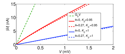
Figure 2: The RG-improved current correction (Electrical control of the Kondo effect in a helical edge liquid) at $T=30$ mK as a function of applied voltage, for different values of $K_{0}$ and $\theta$. The dashed lines represent $\theta\approx 0.27$, corresponding to $\hbar\alpha=10^{-10}$ eVm. Other parameters are defined in the text. The QSH edge current $G_{0}V$ is plotted as a reference.

Experimental realization. Given our result in Eq. (Electrical control of the Kondo effect in a helical edge liquid), is the Rashba-dependence of $\delta I$ large enough to be seen in an experiment? As a case study, let us consider an Mn²⁺ ion implanted close to the edge of an HgTe quantum well Datta . Mn²⁺ has spin $S\!=\!5/2$, but, due to the large and positive single-ion anisotropy $\propto(S^{z})^{2}$ at the quantum well interface, the higher spin components freeze out in the sub-Kelvin range, leaving behind a spin-1/2 doublet Ujsaghy . Moreover, the single-ion anisotropy implies that the Kondo interaction with this effective spin-1/2 impurity is anisotropic, with $J_{x}=J_{y}=3J_{z}=3J_{I}$, where $J_{I}$ is the isotropic bulk spin-exchange coupling Zitko . Its value can be assessed from the sp-d exchange integrals for the bulk conduction electrons in Hg_1-xMn_xTe Furdyna . Close to the $\Gamma$-point of the Brillouin zone these integrals produce an antiferromagnetic exchange, $J_{I}>0$. With the Mn²⁺ ion located within the penetration depth $\kappa$ from the edge, a rough estimate yields an expected value of $J_{I}/a_{0}\approx 10$ meV, with $a_{0}$ the lattice constant. Turning to the Rashba coupling $\alpha$, gate controls have been demonstrated in the laboratory with $\hbar\alpha$ for an HgTe quantum well device running from $5\times 10^{-11}$ eVm to $1\times 10^{-10}$ eVm as the bias of a top gate is varied from 2 V to -2 V Hinz . As for the value of the interaction parameter $K_{0}$ in an HgTe quantum well, estimates range between 0.5 and 1 M ; Strom ; Hou ; Strom2 ; TeoKane , and depend on the geometry and composition of the heterostructure. Collecting the numbers, and putting $a_{0}\approx 0.5$ nm Efros , $v_{F}\approx 5.0\times 10^{5}$ m/s Konig , and $D\approx 300$ meV Konig , we can use Eq. (Electrical control of the Kondo effect in a helical edge liquid) to numerically plot the $\delta I$-$V$ characteristics for different values of $\alpha$ and $K_{0}$ footnote , choosing $T=30$ mK ($>$$T_{K}$), see Fig. (2). As revealed by the graphs, the Rashba-dependence of $\delta I$ should allow for an experimental test footnote2 .

Concluding remarks. We have studied the combined effect of a Kondo and a Rashba interaction at the edge of a quantum spin Hall system. The interplay between an anisotropic Kondo exchange and the Rashba interaction is found to result in a non-collinear electron-impurity spin interaction. A perturbative RG analysis indicates that this interaction may block the Kondo effect when the electron-electron interaction is weakly screened. We conjecture that this surprising result $-$ challenging a time-honored expectation that the Kondo effect is blind to time-reversal invariant perturbations Meir $-$ is due to the breakdown of single-particle physics in one dimension. It remains a challenge to unravel the microscopic scenario behind this intriguing phenomenon. In the second part of our work we derived expressions showing how charge transport at the edge is influenced by the simultaneous presence of a magnetic impurity and a Rashba interaction. A case study suggests that the predicted current-voltage characteristics should indeed be accessible in an experiment. Most interestingly, its manifest dependence on the gate-controllable Rashba coupling breaks a new path for charge control in a helical electron system.

Acknowledgments. It is a pleasure to thank S. Eggert, D. Grundler, C.-Y. Hou, G. I. Japaridze, P. Laurell, T. Ojanen, and D. Schuricht for valuable discussions. We also thank F. Crépin and P. Recher for drawing our attention to an erroneous expression for the current operator in an earlier version of this paper erratum . This research was supported by the Swedish Research Council (Grant No. 621-2011-3942) and by STINT (Grant No. IG2011-2028).

Appendix A Supplemental Material

In this supplementary material we derive the conductance correction $\delta G(\omega)$ as a function of the frequency $\omega$, using a rate equation approach in the spirit of Tanaka et al. [9]. Since the rotated spin-up ($\uparrow^{\prime}$) and spin-down ($\downarrow^{\prime}$) states define right and left movers, the current operator takes the form $\hat{I}=(e/2)\,\partial_{t}\,(\Psi^{\prime\dagger}\sigma^{z^{\prime}}\Psi^{\prime})$ in the rotated basis. A voltage $V=V_{0}e^{-\mathrm{i}\omega t}$ adds a term $H_{V}=(eV/2)\int\mathrm{d}x\,\,\Psi^{\prime\dagger}\sigma^{z^{\prime}}\Psi^{\prime}$ to the Hamiltonian. A rate equation can now be constructed for the impurity spin,

$$\partial_{t}P^{i}_{\uparrow^{\prime}}=(\gamma_{+}+\gamma^{\prime}_{-}+\tilde{\gamma}^{E}_{0})P^{i}_{\downarrow^{\prime}}-(\gamma_{-}+\gamma^{\prime}_{+}+\tilde{\gamma}^{E}_{0})P^{i}_{\uparrow^{\prime}},$$ (S.1)

with $P^{i}_{\uparrow^{\prime},\downarrow^{\prime}}$ the probability of the impurity spin being in the $\uparrow^{\prime}$ or $\downarrow^{\prime}$ state, where $P^{i}_{\uparrow^{\prime}}+P^{i}_{\downarrow^{\prime}}=1$. The solution is

$$P^{i}_{\uparrow^{\prime}}=\frac{1}{2}+\frac{e}{2T}\,\frac{\gamma_{0}-\gamma^{\prime}_{0}}{2(\gamma_{0}+\gamma^{\prime}_{0}+\tilde{\gamma}^{E}_{0})-\mathrm{i}\omega}\,V_{0}e^{-\mathrm{i}\omega t}.$$ (S.2)

The $\gamma$-parameters encode the various voltage-dependent spin-flip rates implied by $H^{\prime}_{K}$ in Eq. (3),

$$\sigma^{\mp}S^{\pm}\to\gamma_{\pm},\quad\sigma^{\pm}S^{\pm}\to\gamma^{\prime}_{\mp},\quad\sigma^{\mp}S^{z^{\prime}}\to\gamma^{E}_{\pm},\quad\sigma^{z^{\prime}}S^{\pm}\to\tilde{\gamma}^{E}_{0}.$$

Here $\gamma_{\pm}=\gamma_{0}\Lambda_{\pm},\gamma^{\prime}_{\pm}=\gamma^{\prime}_{0}\Lambda_{\pm},\gamma^{E}_{\pm}=\gamma^{E}_{0}\Lambda_{\pm}$, with $\Lambda_{\pm}\equiv 1\pm eV/2T$ for $eV\ll T$, where the rates $\gamma_{0}$, $\gamma^{\prime}_{0}$, $\gamma_{0}^{E}$ and $\tilde{\gamma}_{0}^{E}$ are determined below.

The current correction $\delta I=I-G_{0}V$ due to the impurity is given by

$$\delta I=-e\,\big{(}\gamma_{+}P^{i}_{\downarrow^{\prime}}-\gamma^{\prime}_{-}P^{i}_{\downarrow^{\prime}}+\gamma^{\prime}_{+}P^{i}_{\uparrow^{\prime}}-\gamma_{-}P^{i}_{\uparrow^{\prime}}+\gamma^{E}_{+}/2-\gamma^{E}_{-}/2\big{)}.$$ (S.3)

Combining Eqs. (S.2) and (S.3) gives for the conductance correction, $\delta G(\omega)=\delta I/(V_{0}e^{-\mathrm{i}\omega t})$,

$$\delta G(\omega)=-\frac{e^{2}}{2T}\Big{[}\frac{(\gamma_{0}+\gamma^{\prime}_{0}+\gamma_{0}^{E})\omega+\mathrm{i}8\gamma_{0}\gamma^{\prime}_{0}+\mathrm{i}2(\gamma_{0}+\gamma^{\prime}_{0})(\gamma_{0}^{E}+\tilde{\gamma}_{0}^{E})+\mathrm{i}2\tilde{\gamma}_{0}\gamma_{0}^{E}}{\mathrm{i}2(\gamma_{0}+\gamma^{\prime}_{0}+\tilde{\gamma}_{0}^{E})+\omega}\Big{]}.$$ (S.4)

In the dc limit, i.e. $\omega\ll J^{2}\ll T$, we then obtain

$$\delta G(\omega\to 0)=-\frac{e^{2}}{2T}\Big{[}\frac{4\gamma_{0}\gamma^{\prime}_{0}\!+\!(\gamma_{0}\!+\!\gamma^{\prime}_{0})(\gamma_{0}^{E}\!+\!\tilde{\gamma}_{0}^{E})\!+\!\tilde{\gamma}^{E}_{0}\gamma_{0}^{E}}{\gamma_{0}\!+\!\gamma^{\prime}_{0}\!+\!\tilde{\gamma}_{0}^{E}}\Big{]}.$$ (S.5)

The rates $\gamma_{0}$, $\gamma^{\prime}_{0}$ and $\gamma_{0}^{E}$ are now determined by considering the regime $\gamma_{0}$,$\gamma^{\prime}_{0}$,$\gamma_{0}^{E}$,$\tilde{\gamma}_{0}^{E}\ll\omega\ll T$, where Eq. (S.4) gives

$$\delta G(\omega\gg\gamma)=-\frac{e^{2}}{2T}\big{(}\gamma_{0}+\gamma^{\prime}_{0}+\gamma_{0}^{E}\big{)}.$$ (S.6)

Comparing Eq. (S.6) with the linear-response result in Eq. (11) immediately gives $\gamma_{0}\sim(J_{x}+J_{y}^{\prime})^{2}T^{2(\sqrt{K}-\lambda/2)^{2}-1}$, $\gamma_{0}^{\prime}\sim(J_{x}-J_{y}^{\prime})^{2}T^{2(\sqrt{K}+\lambda/2)^{2}-1}$, and $\gamma_{0}^{E}\sim J_{E}^{2}T^{2K-1}$.

Obtaining $\tilde{\gamma}_{0}^{E}$ requires some additional work, since the terms $\sigma^{z^{\prime}}S^{-}$ and $\sigma^{z^{\prime}}S^{+}$ in $H^{\prime}_{K}$, Eq. (3), do not backscatter electrons. Hence the rate $\tilde{\gamma}_{0}^{E}$ does not enter the linear-response conductance result in Eq. (11). To make progress one may introduce an auxiliary field coupling to the impurity instead of the electrons. A suitable choice is to apply a magnetic field $h=h_{0}e^{-\mathrm{i}\omega t}$ to the impurity spin and obtain the spin-flip rates when $h\to 0$ using linear response. The equilibrium probabilities for the impurity spin are then

$$P^{i}_{\uparrow^{\prime},\downarrow^{\prime}}=\frac{e^{\pm\mu h/2T}}{e^{\mu h/2T}+e^{-\mu h/2T}},$$ (S.8)

and the spin-flip rates induced by $H^{\prime}_{K}$ now correspond to

$$\sigma^{\mp}S^{\pm}\to\gamma_{\pm},\quad\sigma^{\pm}S^{\pm}\to\gamma^{\prime}_{\pm},\quad\sigma^{\mp}S^{z^{\prime}}\to\gamma^{E}_{0},\quad\sigma^{z^{\prime}}S^{\pm}\to\tilde{\gamma}^{E}_{\pm},$$

with $\gamma_{\pm}=\gamma_{0}\Lambda_{\pm},\gamma^{\prime}_{\pm}=\gamma^{\prime}_{0}\Lambda_{\pm},\tilde{\gamma}^{E}_{\pm}=\tilde{\gamma}^{E}_{0}\Lambda_{\pm}$, where we now have $\Lambda_{\pm}\equiv 1\pm\mu h/2T$ in the limit $\mu h\ll T$. Since the ballistic conduction electrons are in equilibrium with the leads, the rate equation for the impurity spin can be written as

$$\partial_{t}P^{i}_{\uparrow^{\prime}}=\frac{1}{2}\big{[}-\gamma_{-}+\gamma_{+}+\gamma^{\prime}_{+}-\gamma^{\prime}_{-}-\tilde{\gamma}^{E}_{-}+\tilde{\gamma}^{E}_{+}\ \big{]}=\frac{\mu h}{2T}\big{(}\gamma_{0}+\gamma^{\prime}_{0}+\tilde{\gamma}_{0}^{E}\big{)}.$$ (S.9)

This gives the "spin-flip susceptibility", $\chi\equiv\partial(\partial_{t}P^{i}_{\uparrow^{\prime}})/\partial(\mu h)$,

$$\chi=\frac{1}{2T}\big{(}\gamma_{0}+\gamma^{\prime}_{0}+\tilde{\gamma}_{0}^{E}\big{)}.$$ (S.10)

The rate $\tilde{\gamma}_{0}^{E}$ can now be extracted from a linear response calculation. The operator $\partial_{t}S^{z^{\prime}}$, given by $\partial_{t}S^{z^{\prime}}=(\mathrm{i}\hbar)^{-1}\,\big{[}S^{z^{\prime}},H^{\prime}_{K}\big{]}$, becomes

$$\partial_{t}S^{z^{\prime}}\ =\ \frac{\mathrm{i}}{\hbar}\frac{1}{2\pi\kappa}\sum_{j=\pm}\left(\frac{J_{x}+jJ^{\prime}_{y}}{2}\right)e^{\mathrm{i}(2\sqrt{K}-j\lambda)\varphi(0)}S^{j}\ -\ \frac{1}{\hbar}\frac{J_{E}}{2}\frac{1}{\pi\sqrt{K}}:\partial_{x}\vartheta(0)e^{-\mathrm{i}\lambda\varphi(0)}:S^{+}\ +\ h.c..$$ (S.11)

Calculating the "spin-flip susceptibility" $\chi$ using the Kubo formula, $\chi(\omega)=(\hbar\omega)^{-1}\int_{0}^{\infty}\mathrm{d}t\,e^{\mathrm{i}\omega t}\langle\big{[}(\partial_{t}S^{z^{\prime}})^{\dagger}(t),\partial_{t}S^{z^{\prime}}(0)\big{]}\rangle$, in the regime $\gamma_{0}$,$\gamma^{\prime}_{0}$,$\tilde{\gamma}_{0}^{E}$,$\tilde{\gamma}_{0}^{E}\ll\omega\ll T$, we get

$$\chi\ =\ \,\frac{1}{\hbar}\sum_{j=\pm}\Bigg{[}\frac{J_{x}+jJ^{\prime}_{y}}{2}\Bigg{]}^{2}F_{j}\cdot\left(\frac{2\pi T}{D}\right)^{2(\sqrt{K}-j\lambda/2)^{2}-2}+\frac{1}{\hbar}\Bigg{[}\frac{J_{E}}{2}\Bigg{]}^{2}\mu.$$ (S.12)

with $\mu=(1+\lambda^{2}/2)\sin(\pi\lambda^{2}/4)/(\pi\hbar v\sqrt{K})^{2}$. Comparing Eqs. (S.10) and (S.12) we once again see that $\gamma_{0}\sim(J_{x}+J_{y}^{\prime})^{2}T^{2(\sqrt{K}-\lambda/2)^{2}-1}$ and $\gamma_{0}^{\prime}\sim(J_{x}-J_{y}^{\prime})^{2}T^{2(\sqrt{K}+\lambda/2)^{2}-1}$, and now we can also conclude that $\tilde{\gamma}_{0}^{E}\sim J_{E}^{2}T$ .

Thus we have obtained all rates appearing in the the conductance $\delta G(\omega)$ in Eq. (S.4).

References

(1)
M. König et al., Science 318, 766 (2007).
(2)
For a review, see X.-L. Qi and S.-C. Zhang, Rev. Mod. Phys. 83, 1057 (2011).
(3) C. Wu et al., Phys. Rev. Lett. 96, 106401 (2006).
(4) C. Xu and J. E. Moore, Phys. Rev. B 73, 045322 (2006).
(5)
D. Meidan and Y. Oreg, Phys. Rev. B 72, 121312(R) (2005).
(6)
T.L. Schmidt et al., Phys. Rev. Lett. 108 156402 (2012).
(7)
N. Lezmy et al., Phys. Rev. B 85 235304 (2012).
(8)
J. Maciejko et al., Phys. Rev. Lett. 102 256803 (2009).
(9)
Y. Tanaka et al., Phys. Rev. Lett. 106 236402 (2011).
(10)
R. Winkler, Spin-Orbit Interaction Effects in Two-Dimensional Electron and Hole Systems
(Springer, Berlin, 2003).
(11)
H. Buhmann, J. Appl. Phys. 109, 102409 (2011).
(12)
B. A. Bernevig et al., Science 314, 1757 (2006).
(13)
C. L. Kane and E. J. Mele, Phys. Rev. Lett. 95, 226801 (2005).
(14)
A. Ström et al., Phys. Rev. Lett. 104, 256804 (2010).
(15)
Y. Meir and N. S. Wingreen, Phys. Rev. B 50, 4947 (1994).
(16)
O. Újsághy and A. Zawadowski, Phys. Rev. B 57, 11598 (1998).
(17)
R. Žitko et al., Phys. Rev. B 78, 224404 (2008).
(18)
J. I. Väyrynen and T. Ojanen, Phys. Rev. Lett. 106, 076803 (2011).
(19)
J. C. Budich et al., Phys. Rev. Lett. 108, 086602 (2012).
(20)
T. Giamarchi, Quantum Physics in One Dimension (Oxford University Press, Oxford, 2003).
(21)
C. L. Kane and M. P. A. Fisher, Phys. Rev. B 46, 15233 (1992).
(22)
J. Maciejko, Phys. Rev. B 85, 245108 (2012).
(23)
M. Pletyukhov and D. Schuricht, Phys. Rev. B 84, 041309(R) (2011).
(24)
X.-Y. Feng and F.-C. Zhang, J. Phys. Condens. Matter 23, 105602 (2011).
(25)
R. Žitko and J. Bonča, Phys. Rev. B 84, 193411 (2011).
(26)
M. Zarea et al., Phys. Rev. Lett. 108, 046601 (2012).
(27)
L. Isaev et al., Phys. Rev. B 85, 081107 (2012).
(28)
The position of the ”dome” in Fig. (1) is determined by the condition that the magnitude of the scale-dependent
amplitude of the non-collinear term outgrows , , and under RG.
Note that when , this does not happen since now will be large for large ,
making dominate the RG flow.
(29)
J. Malecki, J. Stat. Phys. 129, 741 (2007).
(30)
G. Mahan, Many-Particle Physics (Kluwer Academic / Plenum Publishers, New York, 2000).
(31)
X.-G. Wen, Phys. Rev. B 44 5708 (1991).
(32)
S. Datta et al.,
Superlattice Microst. 1, 327 (1985).
(33)
J. K. Furdyna, J. Appl. Phys. 64, R29 (1988).
(34)
J. Hinz et al., Semicond. Sci. Technol. 21, 501 (2006).
(35)
C.-Y. Hou et al., Phys. Rev. Lett. 102, 076602 (2009).
(36)
A. Ström and H. Johannesson, Phys. Rev. Lett. 102, 096806 (2009).
(37)
J. C. Y. Teo and C. L. Kane, Phys. Rev B 79, 235321 (2009).
(38) A. L. Efros and B. I. Shklovskii, Electronic Properties of
Doped Semiconductors (Springer, Heidelberg, 1989).
(39)
Since in Eq. (3) is RG-relevant (marginally relevant) for , the
condition for perturbation theory to be valid restrains to values
close to unity in the chosen voltage interval.
(40)
Note that a test requires the concurrent tunability of a back gate, so as to keep the electron density fixed Grundler .
(41)
D. Grundler, Phys. Rev. Lett. 84, 6074 (2000).
(42)
The corrections in the present version, including the new Fig. 2, will be published in an Erratum to
Phys. Rev. B 86, 161103(R) (2012).