Fingerprints of spin-orbital entanglement in transition metal oxides

Abstract

The concept of spin-orbital entanglement on superexchange bonds in transition metal oxides is introduced and explained on several examples. It is shown that spin-orbital entanglement in superexchange models destabilizes the long-range (spin and orbital) order and may lead either to a disordered spin-liquid state or to novel phases at low temperature which arise from strongly frustrated interactions. Such novel ground states cannot be described within the conventionally used mean field theory which separates spin and orbital degrees of freedom. Even in cases where the ground states are disentangled, spin-orbital entanglement occurs in excited states and may become crucial for a correct description of physical properties at finite temperature. As an important example of this behaviour we present spin-orbital entanglement in the $R$VO₃ perovskites, with $R$=La,Pr,$\cdots$,Yb,Lu, where such finite temperature properties of these compounds can be understood only using entangled states: ($i$) thermal evolution of the optical spectral weights, ($ii$) the dependence of transition temperatures for the onset of orbital and magnetic order on the ionic radius in the phase diagram of the $R$VO₃ perovskites, and ($iii$) dimerization observed in the magnon spectra for the $C$-type antiferromagnetic phase of YVO₃. Finally, it is shown that joint spin-orbital excitations in an ordered phase with coexisting antiferromagnetic and alternating orbital order introduces topological constraints for the hole propagation and will thus radically modify transport properties in doped Mott insulators where hole motion implies simultaneous spin and orbital excitations.

Published in: Journal of Physics: Condensed Matter 24, 313201 (2012).

1 Introduction: Entanglement in many-body systems

Superexchange models with spin-orbital entanglement on superexchange bonds, discovered by exact diagonalization of finite chains [1], are a good recent example of entanglement in many-body systems. Entanglement is inherent to quantum mechanics and occurs in several systems. In general it means that quantum states have internal structure and cannot be represented as products of states which belong to different subspaces of the full Hilbert space [2, 3, 4]. This property of quantum states has gained renewed interest in recent years as it was found in several many-body quantum systems and it was realized that it may play a role in quantum information. It is shown below that it leads to measurable consequences in condensed matter systems with strongly correlated electrons, when orbital degrees of freedom are active. This new development concerns both model systems and the physical properties of Mott (or charge transfer) insulators — we summarize it shortly in the present topical review.

Entanglement in quantum many-body systems is a broad field [3] and will not be discussed here as such. In the last few decades the interest in quantum entanglement has risen sharply in various formerly disconnected subfields of physics. At present these different communities come closer to each other in the search for universal ways of quantifying entanglement and developing algorithms to treat many-body quantum systems. An interested reader is encouraged to consult several review articles published recently on this subject — we name here only a few which focus on entanglement in: ($i$) many-body systems [5], ($ii$) quantum spin systems [6], ($iii$) interacting fermionic and bosonic many-particle systems [7], ($iv$) optical lattices [8], and finally, ($v$) quantum cryptography and quantum communication [4]. Entanglement entropy plays a central role in these systems and is frequently used as a quantitative measure of entanglement [9].

Spin-orbital entanglement occurs either due to the relativistic on-site spin-orbit coupling or due to superexchange interactions on the bonds. While finite spin-orbit coupling introduces on-site entanglement, a qualitatively new and challenging situation is encountered when degenerate $3d$ orbitals of transition metal ions are partly filled and orbital degrees of freedom have to be treated on equal footing with electron spins in the effective spin-orbital superexchange model [10]. Here we mainly on the latter but some recent examples of entangled states in cases with strong spin-orbit coupling will also be mentioned for completeness at the end.

When degenerate $3d$ orbitals in a transition metal oxide are partly filled, realistic superexchange includes both orbital and spin degrees of freedom that are strongly interrelated [10, 11]. The microscopic models designed to describe realistic systems with strongly correlated and partly localized electrons include as well orbital interactions which follow from the orbital-lattice coupling and tune the orbital correlations. These latter interactions are rather strong in the $e_{g}$ orbital systems and stabilize the orbital order at rather high temperature, as for instance in LaMnO₃ [12]. It such cases it is well justified to treat the spin-orbital superexchange in the mean field (MF) approximation which separates orbital degrees of freedom and their dynamics from the spin ones [13]. The spin and orbital degrees of freedom order then in a complementary way and their order follows the classical Goodenough-Kanamori rules [14]. They were derived long ago from the microscopic insights concerning the structure of spin-orbital superexchange and predict that the antiferromagnetic (AF) order coexists with ferro-orbital (FO) order and ferromagnetic (FM) order coexists with alternating orbital (AO) order. Out of many examples which follow these rules, we mention here only the LaMnO₃ perovskite, with active $e_{g}$ orbitals and coexisting FM/AO order in $ab$ planes and AF/FO order along the $c$ axis [12, 15]. In this case spin and orbital operators indeed separate as the orbital order sets in at high temperature $T_{\rm OO}=780$ K and is already saturated when the $A$-type AF ($A$-AF) order occurs at $T_{\rm N}\simeq 140$ K. Therefore, the optical spectral weights measured in experiment are well described by the MF decoupling of spin and orbital degrees of freedom [16]. For this reason simple treatments of the models of manganites which use the MF approach [17, 18] or Hartree-Fock decoupling [19] are very successful in modeling the complex phase diagram of monolayer, bilayer and cubic manganites [20].

In a number of compounds with active orbital degrees of freedom where strong on-site Coulomb interactions localize electrons (or holes) and give rise to spin-orbital superexchange, two different types of long-range order compete with each other. A prominent example of this behaviour are the $R$VO₃ perovskites, where $R$=Lu,Yb,$\cdots$,La. In the case of perovskite vanadates the cubic symmetry is broken by GdFeO₃-like distortions and the $xy$ orbitals are singly occupied at all V³⁺ ions, while the second electron occupies the $\{yz,zx\}$ doublet. One finds here two different AF phases for V³⁺ ions in $d^{2}$ electronic configuration with $S=1$ spin: ($i$) the $C$-type AF ($C$-AF) phase with staggered AF order in the $ab$ planes accompanied by the FM order along the $c$ axis, coexisting with weak AO order of active $t_{2g}$ orbitals $\{yz,zx\}$, and ($ii$) the $G$-type AF ($G$-AF) phase with staggered AF order along all three cubic axes coexisting with robust $C$-type orbital order [21]. In fact, the coexisting orbital and magnetic order in these phases obey the Goodenough-Kanamori rules along the $c$ axis. However, the situation in $ab$ planes of this class of compounds is puzzling as two alternating orders coexist, both for spins and for orbitals. The reasons of this coexistence are more subtle — there also $xy$ orbitals are singly occupied at every ion and they are in a FO state, while the spin order, driven mainly by them, is AF. So once again, the order in the $ab$ planes can be understood using the Goodenough-Kanamori rules. However, the AF/AO order may be seen as entangled in the subspace of $\{yz,zx\}$ orbitals and provides an interesting situation in doped systems, as we shall discuss below.

Recent interest and theoretical progress in the understanding of spin-orbital superexchange models was triggered by the observation that orbital degeneracy significantly enhances quantum fluctuations which may even suppress long-range order when different types of symmetry broken states compete with each other near the quantum critical point [22]. The simplest and paradigmatic model in this context is the Kugel-Khomskii model introduced long ago for KCuF₃ [10], a strongly correlated insulator with a single hole within degenerate $e_{g}$ orbitals at Cu²⁺ ions in the $d^{9}$ electronic configuration. This model has two parameters which favour different types of symmetry broken states: ($i$) Hund’s exchange interaction, and ($ii$) the crystal field splitting of $e_{g}$ orbitals. When both these parameters are small the system is driven by its quantum nature — either long-range order disappears [22, 23] or, for certain parameters, coexisting spin and orbital order might be stabilized by order out of disorder mechanism [24]. We shall discuss below to what extent the order is classical and show that spin-orbital entanglement manifests itself in the regime of most frustrated interactions.

First, in this topical review we shall elucidate certain situations with the spin-orbital entanglement in the ground states (GSs). Such GSs are very challenging as there are no good methods in the theory to investigate them in a systematic way. It will become evident that quite different GSs arise, characterized by overestimated energy and incorrect correlation functions, when spin-orbital entanglement is neglected.

Second, even when the GSs are not entangled, entanglement may be experimentally observed and has important consequences at finite temperature when the behaviour of the system is driven by low-energy excited states with spin-orbital entanglement. The existence of such states is a generic feature of any spin-orbital superexchange model and therefore the relevant question is only whether such states are accessible for thermal excitations. It will be shown that a rather exotic behaviour of the $R$VO₃ perovskites cannot be understood without including the spin-orbital entangled states. This point of view is supported by several experimental observations: ($i$) the thermal evolution of the optical spectral weights [25], ($ii$) the phase diagram of the $R$VO₃ perovskites [21], and ($iii$) the observed dimerization in the magnon spectra of YVO₃ [26].

An interesting situation arises also in doped Mott insulators, where doped holes introduce charge degrees of freedom which perturb the orbital order and frequently lead to phases with coexisting spin, charge and orbital order [27]. When orbital degrees of freedom are quenched, one finds that hole propagation occurs in the $t$-$J$ model via a quasiparticle state that emerges due to quantum fluctuations in the spin background [28]. In $t$-$J$-like superexchange models with orbital degrees of freedom, hole propagation is either entirely suppressed by incoherent processes [29], or occurs by a rather subtle mechanism: either by off-diagonal orbital hopping in $e_{g}$ orbital systems [30], or by next-nearest neighbour effective hopping in $t_{2g}$ systems [31, 32]. When both spin and orbital degrees of freedom may contribute, the situation is less clear as scattering on spin-flip processes introduces additional incoherence in hole propagation [33]. Surprisingly, it was realized only recently that spin-orbital entanglement introduces topological constraints for hole propagation in a Mott insulator with coexisting AF and AO order [34], and may thus have serious measurable consequences in doped $R$VO₃ perovskites.

The paper is organized as follows. In section 2 we explain general concepts of: ($i$) intrinsic frustration of orbital interactions, ($ii$) spin-orbital superexchange, and ($iii$) its consequences for the magnetic exchange constants and the optical spectral weights. Next we describe spin-orbital entanglement in the GSs of spin-orbital models in section 3. Such models are usually employed to explain the magnetic properties of transition metal oxides [13] and are also used to derive the optical spectral weights [35]. Therefore, even when the GSs are disentangled, entangled states have severe consequences on the experimentally observed properties of some Mott insulators at finite temperature, and we describe in section 4 the properties of the perovskite $R$VO₃ systems as an example of such a complex behaviour driven by quantum entanglement. Spin-orbital entanglement may also occur in GSs in particular parameter regimes, and we provide two examples of this behaviour in section 5: ($i$) the Kugel-Khomskii model on a bilayer [36], and ($ii$) the $d^{1}$ model for $t_{2g}$ electrons on a triangular lattice [37, 38]. Entangled states may have also interesting consequences for hole propagation in ordered states — here we present the coupling of a hole to joint spin-orbital excitations [34], see section 6. The paper is concluded in section 7, where a general discussion and main conclusions are presented.

2 Orbital and spin-orbital superexchange

2.1 Intrinsic frustration of orbital interactions

Before presenting the spin-orbital entanglement, we first introduce the characteristic features of orbital superexchange interactions as obtained in case of spin polarized (FM) systems. These interactions are fundamentally different from spin superexchange which has high SU(2) symmetry and intrinsically frustrated. Frustration is one of the simplest concepts in physics with far reaching consequences [39, 40]. The main and unusual feature of orbital interactions is their intrinsic frustration that follows from the directional nature of superexchange terms which contribute along different bonds and compete with one another [22]. This type of frustration does not follow from geometrical frustration and is best understood by considering a two-dimensional (2D) square lattice. In case of the Ising model frustration on a square lattice can be achieved, for instance, by changing signs of interactions along every second column and leaving the other interactions unchanged. In this case all plaquettes of the 2D lattice are frustrated as one of the interactions has the wrong sign but the spins order — the model is exactly solvable and has long-range order following the dominating interaction below a finite transition temperature [41], being lower than the one of the 2D Ising model. We emphasize that this frustrated model is exactly solvable because it is still classical as the interactions concern only commuting $\{S_{i}^{z}\}$ spin components.

In contrast, the orbital interactions on a pseudocubic lattice are quantum, both for $e_{g}$ and $t_{2g}$ orbitals, because they involve at least two pseudospin components [42]. Such models have different (typically cubic) symmetry from both the Z₂ symmetry of Ising and SU(2) symmetry of Heisenberg model, and are in general not exactly solvable on a 2D square lattice. We begin with the case of $e_{g}$ orbitals interacting within a 2D $ab$ plane of K₂CuF₄ compound; models for three-dimensional (3D) perovskites, for instance KCuF₃ with $d^{9}$ electronic configurations of Cu²⁺ ions or LaMnO₃ with $d^{4}$ configurations of Mn³⁺ ions discussed below can be easily obtained as a straightforward generalization of the 2D model using the cubic symmetry of orbital interactions [43]. Two $e_{g}$ orbital states,

$$|z\rangle\equiv\frac{1}{\sqrt{6}}\left(3z^{2}-r^{2}\right),\hskip 28.45274pt|x\rangle\equiv\frac{1}{\sqrt{2}}\left(x^{2}-y^{2}\right),$$ (1)

are the eigenstates of the $\tau^{(c)}_{i}=\frac{1}{2}(n_{iz}-n_{ix})$ orbital operator for pseudospin $\tau=\frac{1}{2}$, where $\{n_{iz},n_{ix}\}$ are hole number operators at site $i$.

The origin of intrinsic frustration in the $e_{g}$ orbital superexchange is best realized by considering its form [43],

$$H_{eg}=J_{\rm orb}\sum_{\langle ij\rangle\parallel\gamma}\left(\tau^{(\gamma)}_{i}\tau^{(\gamma)}_{j}-{1\over 4}\right)\,,$$ (2)

where the bond is oriented along one of the cubic axes $\gamma=a,b,c$ [43]. Here the orbital interaction $J_{\rm orb}>0$ follows from the energy of the high-spin charge excitation [13]. The pseudospin operators take a different form depending on the bond direction and are defined as follows,

$$\tau^{(a,b)}_{i}={1\over 4}\left(-\sigma^{z}_{i}\pm\sqrt{3}\sigma^{x}_{i}\right),\hskip 28.45274pt\tau^{(c)}_{i}={1\over 2}\sigma^{z}_{i},$$ (3)

where $\sigma^{x(z)}_{i}$ are Pauli matrices and the sign $\pm$ in $\tau^{(a,b)}_{i}$ is selected for a bond $\langle ij\rangle$ along $a$ ($b$) axis. Thus for the $ab$ plane one has two linear combinations of $\{\sigma^{x}_{i},\sigma^{z}_{i}\}$ Pauli matrices, and these interactions favour AOs on each bond, being the eigenstates of the $\sigma^{x}_{i}$ Pauli matrix as the interactions $\propto\sigma^{x}_{i}\sigma^{x}_{j}$ are here the strongest ones. We emphasize that the interactions in equation (2) are fundamentally different from the SU(2)-symmetric spin interactions, as they: ($i$) obey only lower cubic symmetry, ($ii$) are Ising-like and select only one component of the pseudospin interaction along each bond which favours pairs of orthogonal orbitals, i.e., oriented along the bond ($z$-like) and the orthogonal to it lying in the plane perpendicular to the bond ($x$-like). This manifests the intrinsic frustration of orbital interactions in the $e_{g}$ orbital case [22]. In fact, the interactions in equation (2) are Ising-like and classical only in the one-dimensional (1D) model [44], but in general they are not. However, due to the gap which opens in orbital excitations in the 2D model, the quantum corrections generated by them are rather small [43].

The essence of orbital frustration which characterizes the $e_{g}$ orbital superexchange (2) is captured by the 2D compass model [45] which arises by increasing frustration from the 2D $e_{g}$ orbital model to the maximal frustration [46]. One considers then the 2D model (or an exactly solvable model compass ladder [47]) that interpolates between the classical Ising one and the compass one passing through the $e_{g}$ orbital model. The orbital interactions $J_{\rm orb}$ are equal along both rows and columns but select two orthogonal pseudospin components [45, 48]:

$$H_{2D}=J\sum_{\langle ij\rangle\parallel a}\tau^{x}_{i}\tau^{x}_{j}+J\sum_{\langle ij\rangle\parallel b}\tau^{z}_{i}\tau^{z}_{j}\,.$$ (4)

Usually one considers the AF case ($J>0$) but the FM model ($J<0$) is equivalent and equally frustrated. Intersite interactions in the 2D compass model are descibed by products $\tau^{\alpha}_{i}\tau^{\alpha}_{j}$ of pseudospin components with $\alpha=x,y,z$,

$$\tau^{x}_{i}=\frac{1}{2}\sigma^{x}_{i},\hskip 28.45274pt\tau^{y}_{i}=\frac{1}{2}\sigma^{y}_{i},\hskip 28.45274pt\tau^{z}_{i}=\frac{1}{2}\sigma^{z}_{i},$$ (5)

rather than by pseudospin scalar products ${\vec{\tau}}_{i}\cdot{\vec{\tau}}_{j}$. As explained below, such scalar products arise for the superexchange interactions with active $t_{2g}$ orbitals degrees of freedom which allow hopping processes for a pair of them in each 2D plane in the cubic system. Instead in the compass model (4) the $\tau^{x}_{i}\tau^{x}_{j}$ interactions for bonds $\langle ij\rangle$ along the $a$ axis compete with the $\tau^{z}_{i}\tau^{z}_{j}$ ones along the $b$ axis [48]. Also the 1D compass model with alternating $\tau^{z}_{i}{2i}\tau^{z}_{2i+1}$ and $\tau^{x}_{2i-1}\tau^{x}_{2i}$ interactions [49] is intrinsically frustrated.

Recently the 2D compass model was investigated by Monte Carlo simulations and the existence of a phase transition at finite temperature was established [50]. The ordered GS is degenerate and its different states correspond to either eigenstates of $\{\tau^{x}_{i}\}$ pseudospin components ordered along the rows, or eigenstates of pseudospin $\{\tau^{z}_{i}\}$ components ordered along the columns [51]. Although this GS is destabilized by infinitesimal pseudospin interactions, the structure of the lowest excited states stays unchanged and corresponds to the flips of spin columns [52]. It has been suggested that the model could serve as an effective model for protected qubits and such states realized by Josephson arrays [53] could play a role in quantum communication. Indeed, first experimental successes in constructing special networks of Josephson junctions that are designed following the compass model were reported recently [54].

Although frustration still increases by going from the 2D to 3D $e_{g}$ orbital model, there are indications from recent Monte Carlo simulations that the GS is ordered [55, 56]. Disorder occurs here by doping which leads to the 3D orbital liquid state [57] that plays a prominent role in the FM metallic manganites and provides an explanation for the observed magnon dispersion [58]. The case of the 3D compass model is more subtle. It was concluded from the high temperature expansion that the ordered state is excluded here [59], but this result was challenged recently [55] and further studies are needed to establish whether this model could indeed serve as an example of an orbital liquid phase.

The orbital models for $t_{2g}$ orbitals contain more terms and were less studied up to now. The generic form contains scalar products of two pseudospins $\tau=1/2$ along each direction in the cubic lattice, defined as in equations (5) [60],

$$H_{t2g}=J_{\rm orb}\sum_{\langle ij\rangle}\left({\vec{\tau}}^{\,(\gamma)}_{i}\cdot{\vec{\tau}}^{\,(\gamma)}_{j}-{1\over 4}\right)\,,$$ (6)

where the operators ${\vec{\tau}}^{\,(\gamma)}_{i}\equiv\{\tau^{x}_{i},\tau^{y}_{i},\tau^{z}_{i}\}^{(\gamma)}$ depend on the bond direction, i.e., the pseudospin components are defined here in different subspaces of the Hilbert space, depending on the pair of active $t_{2g}$ orbitals. This form follows from the fact that only two $t_{2g}$ orbitals allow for electron hopping along a given cubic direction $\gamma$, while the third orbital is inactive, see also below and section 4. For finite Hund’s exchange additional terms arise and the orbital state is disordered [61]. A stable orbital ordered state was found here in the 3D orbital model for YTiO₃, when the spins decouple from $t_{2g}$ orbitals in the FM phase [62].

2.2 Spin-orbital superexchange models

In transition metal compounds with large on-site Coulomb interactions charge fluctuations are suppressed and electrons partly localize. This happens when intraorbital Coulomb interaction $U$ is large compared to the effective $d-d$ hopping element $t$, where $t$ is either the $(dd\sigma)$ or $(dd\pi)$ effective $d-d$ hopping element for $e_{g}$ and $t_{2g}$ systems, respectively, that arises via hybridization with ligand orbitals. In the regime of $t\ll U$, correlated (Mott or charge-transfer) insulators arise in undoped compounds, while doping leads to interesting phenomena in strongly correlated electron systems with charge fluctuations only between two neighbouring electronic configurations [63]. Intersite charge excitations may be then treated within perturbation theory, while the hopping processes which do not cost high local Coulomb energy $U$ and occur in doped systems are treated in the restricted Hilbert space. A well known example of this description is the $t$-$J$ model, used widely to describe the physical properties of high-$T_{c}$ superconductors, but derived one decade before their discovery [64].

Here we concentrate on Mott insulators with transition metal ions in $d^{n}$ electronic configuration and active orbital degrees of freedom, where the effective low-energy Hamiltonians contain spin-orbital superexchange, described within spin-orbital models [10, 11]. Such models are derived using the realistic multiplet structure of the excited states of transition metal ions which arise in $d_{i}^{m}d_{j}^{m}\rightleftharpoons d_{i}^{(m+1)}d_{j}^{(m-1)}$ intersite charge excitations. As the multiplet structure depends on the electron number $m$ [65], with some examples given in [13], these models are specific to a given family of compounds. As a representative example we consider here in more detail the case of the $R$VO₃ perovskites (see section 4), with $S=1$ spin stabilized by Hund’s exchange and active $t_{2g}$ orbitals at V³⁺ ions in $d^{2}$ ($m=2$) electronic configuration. In a cubic perovskite all three $t_{2g}$ orbitals are degenerate and the kinetic energy electrons is given by:

$$H_{t}=-t\sum_{\gamma}\sum_{\langle ij\rangle{\parallel}\gamma,\alpha(\gamma),\sigma}\left(d^{\dagger}_{i\alpha\sigma}d_{j\alpha\sigma}+d^{\dagger}_{j\alpha\sigma}d_{i\alpha\sigma}\right),$$ (7)

where $d^{\dagger}_{i\alpha\sigma}$ is electron creation operator for an electron at site $i$ in orbital state $\alpha$ with spin $\sigma=\uparrow,\downarrow$. The summation runs over three cubic axes, $\gamma=a,b,c$, and involves the bonds $\langle ij\rangle\parallel\gamma$ along them. The hopping $t$ results from transitions via an intermediate O($2p_{\pi}$) orbital and conserves the active $t_{2g}$ orbital flavor $\alpha(\gamma)$. Thus the hopping $t$ is an effective $(dd\pi)$ element that originates from two subsequent $d-p$ hopping processes along each V$-$O$-$V bond in the $R$VO₃ perovskite structure. For $e_{g}$ systems the derivation is similar but the effective hopping elements follow from the hybridization with O($2p_{\sigma}$) orbitals. The effective hopping follows from the charge-transfer model with $p-d$ hybridization $t_{pd}$ and charge-transfer energy $\Delta$ [66], and one expects in the present vanadate case $t=t_{pd}^{2}/\Delta\sim 0.2$ eV [67]. Only two $t_{2g}$ orbitals, labelled by $\alpha(\gamma)$, are active along each bond $\langle ij\rangle{\parallel}\gamma$ and contribute to the kinetic energy (7), while the third one lies in the plane perpendicular to the $\gamma$ axis and the hopping via the intermediate oxygen $2p_{\pi}$ (or $2p_{\sigma}$) oxygen orbital is forbidden by symmetry. This justifies a simplified notation used below, with the orbitals defined by the axis direction which is perpendicular to their plane:

$$|a\rangle\equiv|yz\rangle,\hskip 19.91684pt|b\rangle\equiv|zx\rangle,\hskip 19.91684pt|c\rangle\equiv|xy\rangle.$$ (8)

In this case only $t_{2g}$ orbitals are partly filled by electrons, and it suffices to consider local Coulomb interactions between $t_{2g}$ electrons at V³⁺ ions described by the degenerate Hubbard Hamiltonian [68],

$$H_{\rm int} = U\sum_{i\alpha}n_{i\alpha\uparrow}n_{i\alpha\downarrow}+\left(U-\frac{5}{2}J_{H}\right)\sum_{i,\alpha<\beta}n_{i\alpha}n_{i\beta}$$ (9)

$$+ J_{H}\sum_{i,\alpha<\beta}\left(d^{\dagger}_{i\alpha\uparrow}d^{\dagger}_{i\alpha\downarrow}d_{i\beta\downarrow}d_{i\beta\uparrow}+d^{\dagger}_{i\beta\uparrow}d^{\dagger}_{i\beta\downarrow}d_{i\alpha\downarrow}d_{i\alpha\uparrow}\right)$$

$$- 2J_{H}\sum_{i,\alpha<\beta}\vec{S}_{i\alpha}\cdot\vec{S}_{i\beta}\,.$$

Here $n_{i\alpha}=\sum_{\sigma}n_{i\alpha\sigma}$ is the electron density operator in orbital $\alpha=a,b,c$ at site $i$, and spin operators ${\vec{S}}_{i\alpha}=\{S_{i\alpha}^{x},S_{i\alpha}^{y},S_{i\alpha}^{z}\}$ for orbital $\alpha$ at site $i$ are related to fermion operators in the standard way, i.e.,

$$S_{i\alpha}^{+}\equiv d^{\dagger}_{i\alpha\uparrow}d_{i\alpha\downarrow}\,,\hskip 19.91684ptS_{i\alpha}^{z}\equiv\frac{1}{2}(n_{i\alpha\uparrow}-n_{i\alpha\downarrow})\,.$$ (10)

The first term in (9) describes the largest intraorbital Coulomb interaction $U$ for a pair of electrons with antiparallel spins in orbital $\alpha$. The second term stands for the interorbital Coulomb (density) interaction, the third one is called frequently the ”pair-hopping” term, and the last one is Hund’s exchange $J_{H}$. The choice of coefficients in (9) guarantees that the interactions satisfy the rotational invariance in the orbital space [68]. This Hamiltonian is exact when it describes only one representation of the cubic symmetry group (here $t_{2g}$ orbitals which are partly occupied in the cubic vanadates) — then the on-site interactions are given by two parameters: ($i$) the intraorbital Coulomb element $U$, and ($ii$) Hund’s exchange element $J_{H}$. These elements may be expressed by the Racah parameters $\{A,B,C\}$. For $t_{2g}$ electrons considered in section 4 one finds [13, 65]:

$$U = A+4B+3C\,,$$ (11)

$$J_{H} = 3B+C\,.$$ (12)

Hund’s exchange (and interorbital Coulomb interaction) is in general anisotropic and depends on the pair of interacting orbital states. For instance, the corresponding $e_{g}$ Hund’s exchange element is $J_{H}=4B+C$. More details are given in [13].

In the limit of large $U$ ($t\ll U$), the effective low-energy spin-orbital superexchange interactions arise by considering all the contributions which originate from possible virtual excitations $d_{i}^{m}d_{j}^{m}\rightleftharpoons d_{i}^{m+1}d_{j}^{m-1}$. The general structure of spin-orbital superexchange [13],

$${\cal H}_{J}=J\sum_{\langle ij\rangle}\left\{{\hat{\cal J}}_{ij}^{(\gamma)}\left({\vec{S}}_{i}\cdot{\vec{S}}_{j}+S^{2}\right)+{\hat{\cal K}}_{ij}^{(\gamma)}\right\},$$ (13)

involves interactions between SU(2)-symmetric spin scalar products ${\vec{S}}_{i}\cdot{\vec{S}}_{j}$ on each bond $\langle ij\rangle$, connecting two nearest-neighbor transition metal ions, each one coupled to orbital operators $\{{\vec{\tau}}_{i},{\vec{\tau}}_{j}\}$. The orbital operators are given in section 2.1 and obey only much lower symmetry (at most cubic for a cubic lattice). These operators contribute to the form of orbital operators ${\hat{\cal J}}_{ij}^{(\gamma)}$ and ${\hat{\cal K}}_{ij}^{(\gamma)}$ which depend on the model. They involve the active orbitals on each bond $\langle ij\rangle$ along direction $\gamma$.

In order to derive magnetic excitations for the systems with orbital degeneracy one usually derives magnetic exchange constants for a bond $\langle ij\rangle$ by averaging over the orbital operators in equation (13) using the GS $|\Phi_{0}\rangle$ with decoupled spin and orbital operators,

$$J_{ij}=\langle\Phi_{0}|{\hat{\cal J}}_{ij}^{(\gamma)}|\Phi_{0}\rangle.$$ (14)

This procedure assumes implicitly that spin and orbital operators can be decoupled from each other in the MF approach and ignores the possibility of entanglement and composite spin-orbital excitations introduced in [22]. Inter alia, such excitations play a prominent role in destabilizing the classical AF long-range order in the $d^{9}$ spin-orbital model [23].

The energy scale for the superexchange is given by

$$J=\frac{4t^{2}}{U}.$$ (15)

where $t$ is the relevant effective hopping element and $U$ is the intraorbital Coulomb element defined in (9). As several charge excitations contribute to the superexchange (13), the balance between competing terms depends on Hund’s exchange, namely on

$$\eta=\frac{J_{H}}{U}.$$ (16)

This is the only parameter which decides about the strength of particular interactions in the superexchange and finally also about the type of magnetic correlations or symmetry breaking in the GS obtained at orbital degeneracy and favoured by the model.

We would like to emphasize here that the same charge excitations which decide about the spin-orbital superexchange (13) contribute as well to the optical conductivity. In this case they appear at distinct energies of individual charge excitations that occur at a given ionic filling, and depend on the multiplet structure of the excited states arising from intersite charge transitions [35]. Each of these excitations involves a different intermediate state in the multiplet structure of at least one of the ions after the charge excitation, i.e., either in the $d^{m+1}$ or in the $d^{m-1}$ configuration or in both, depending on the actual process and on the value of $m$ [35]. This feature made it possible to relate the averages of these different excitations to the spectral weights in the optical spectroscopy [35], and this principle serves now as a theoretical tool to analyse and explain the observed anisotropy and temperature dependence of the spectral weights in the optical spectra [13].

As the charge excitations correspond to particular expressions in the spin-orbital space, it is important to rewrite ther superexchange Hamiltonian (13) by decomposing it into individual terms on each bond $\langle ij\rangle$ that stem from particular excited states labeled by $n$ [35],

$${\cal H}_{J}=\sum_{n}\sum_{\langle ij\rangle\parallel\gamma}H_{n}^{(\gamma)}(ij).$$ (17)

Here the superexchange constant (15) was included in the operators $H_{n}^{(\gamma)}(ij)$. As explained above, the spectral weight in the optical spectroscopy is given in a correlated insulator by the same virtual charge excitations that contribute also to the superexchange. They define the individual kinetic energy terms $K_{n}^{(\gamma)}$ along the axis $\gamma$, which can be determined from the superexchange (13) using the Hellman-Feynman theorem [69],

$$K_{n}^{(\gamma)}=-2\big{\langle}H_{n}^{(\gamma)}(ij)\big{\rangle}.$$ (18)

For convenience, we define them here as positive quantities, $K_{n}^{(\gamma)}>0$.

The spectral weights (18) are defined by the bond correlation functions and their changes with increasing temperature which decide about the temperature dependence of the optical spectrum. To describe experimental observations it is therefore important to analyse the various multiplet excitations separately, as they depend on these correlations in a different way, and will also contribute to a quite different temperature dependence, as we show in this paper on the example of LaVO₃ in section 4. Such an analysis is of course possible in each case, as the respective spin-orbital superexchange models are derived by considering all different types of charge excitations individually [13].

In some cases, however, spin dynamics separates from the orbital one in the GS and MF factorization of spin and orbital operators is indeed allowed. This happens when the orbital order is stabilized to a large extent by strong interactions with the lattice which undergoes Jahn-Teller distortions. A good example of this behaviour is LaMnO₃, where the superexchange and the Jahn-Teller effect help each other [12] in stabilizing the orbital order which occurs below the relatively high transition temperature $T_{\rm OO}\simeq 780$ K. The $A$-AF spin order is observed below a much lower Néel temperature $T_{\rm N}\simeq 140$ K [16]. In this case a very satisfactory description of the experimental results for the spectral weight distribution in the optical spectroscopy is obtained using disentangled spin-orbital superexchange, both for the high spin [13] and low spin [16] optical excitations. Below we focus on some examples of a more complex behaviour driven by the spin-orbital entanglement.

3 Spin-orbital entanglement

Before presenting the essence of spin-orbital entanglement, we would like to remind the reader severe consequences of the MF approximation used frequently to investigate spin and/or orbital models. In this approach quantum fluctuations are neglected and only qualitative conclusions concerning possible symmetry breaking can be drawn. In spin-orbital systems the MF approach may be applied in different ways, and here we focus on the decoupling of spin and orbital degrees of freedom presented below for a single bond in section 3.1. When only spin-orbital coupling is treated in the MF approach, spin and orbital operators are disentangled. We show in section 3.2 and section 3.3 that this approximation is unsatisfactory in many situations.

To detect spin-orbital entanglement in the GS we evaluate intersite spin, orbital and joint spin-orbital bond correlations in several models, defined as follows for a nearest-neighbour bond $\langle ij\rangle$ (we keep the notation general here, for the 1D chain $j\equiv i+1$) [1]:

$$S_{ij} \equiv \frac{1}{2S^{2}}\,\langle{\vec{S}}_{i}\cdot{\vec{S}}_{j}\rangle,$$ (19)

$$T_{ij} \equiv \langle{\vec{\tau}}_{i}\cdot{\vec{\tau}}_{j}\rangle,$$ (20)

$$C_{ij} \equiv \frac{1}{2S^{2}}\,\Big{\{}\Big{\langle}({\vec{S}}_{i}\cdot{\vec{S}}_{j})({\vec{\tau}}_{i}\cdot{\vec{\tau}}_{j})\Big{\rangle}-\Big{\langle}{\vec{S}}_{i}\cdot{\vec{S}}_{j}\Big{\rangle}\Big{\langle}{\vec{\tau}}_{i}\cdot{\vec{\tau}}_{j}\Big{\rangle}\Big{\}}.$$ (21)

The above general expressions imply averaging over the exact GS found from Lanczos diagonalization of a finite cluster and are valid for $S=\frac{1}{2}$ and $S=1$ encountered in the models for $t_{2g}$ orbitals investigated in section 3.3. While $S_{ij}$ and $T_{ij}$ correlations indicate the tendency towards particular spin and orbital order, $C_{ij}$ quantifies the spin-orbital entanglement — if $C_{ij}<0$ spin and orbital operators are entangled and the MF approximation, i.e., decoupling of spin and pseudospin operators in (13), cannot be applied as it generates uncontrollable errors.

3.1 Exact versus mean field states for a bond

The spin-orbital superexchange (13) takes the simplest form when Hund’s exchange is absent ($J_{H}=0$) — then the orbital operators $\hat{\cal J}_{ij}^{(\gamma)}$ which couple to the scalar spin product $({\vec{S}}_{i}\cdot{\vec{S}}_{j})$ are particularly simple. In case of $e_{g}$ orbitals they are just projection operators on the active directional orbital [70], while for $t_{2g}$ orbitals they give a scalar product of $\tau=\frac{1}{2}$ pseudospins which represent two active orbital flavours along the bond direction (7). As an example, we consider first a bond in the 1D SU(2)$\otimes$SU(2) model for $S=1$ spins of V³⁺ ions coupled to $\tau=\frac{1}{2}$ pseudospins. Here we show that quantum fluctuations in both spin and orbital system are crucial to reproduce faithfully the energy spectrum of a bond with the spin-orbital superexchange,

$${\cal H}_{12}=\frac{1}{2}J\,\left({\vec{S}}_{1}\cdot{\vec{S}}_{2}+1\right)\left({\vec{\tau}}_{1}\cdot{\vec{\tau}}_{2}+\frac{1}{4}\right).$$ (22)

Such superexchange interactions are obtained in a perovskite $R$VO₃ vanadate along the $c$ axis in absence of Hund’s exchange ($\eta=0$) [71]. The above form is convenient for further discussion and we neglected here a constant term (which would play a role for the optical spectral weights [35]).

While the energy spectrum for a single bond can be easily solved exactly using the SU(2)$\otimes$SU(2) symmetry and the classification of quantum states by the total spin $\vec{\cal S}_{t}\equiv\vec{S}_{1}+\vec{S}_{2}$ and orbital (pseudospin) $\vec{\tau}_{t}\equiv\vec{\tau}_{1}+\vec{\tau}_{2}$ operators, in a solid or in an infinite chain this is not the case and one has to employ some approximation. Frequently the MF theory is used which has severe limitations as the quantum fluctuations on the bonds are then neglected. This can be seen by solving the problem of a single bond (22), either by replacing the scalar products of both spin and orbital operators by their $z$th components (${\cal H}_{12}^{\rm Ising}$), or by treating in the MF approximation only the (more classical) spin scalar product for $S=1$ spins (${\cal H}_{12}^{z}$):

$${\cal H}_{12}^{\rm Ising} = \frac{1}{2}J\,\Big{(}S_{1}^{z}S_{2}^{z}+1\Big{)}\left(\tau_{1}^{z}\tau_{2}^{z}+\frac{1}{4}\right),$$ (23)

$${\cal H}_{12}^{z} = \frac{1}{2}J\,\Big{(}S_{1}^{z}S_{2}^{z}+1\Big{)}\left({\vec{\tau}}_{1}\cdot{\vec{\tau}}_{2}+\frac{1}{4}\right).$$ (24)

Note that the Ising-like Hamiltonian (23) is nonnegative by construction, so the GS energy $E_{0}=0$ is obtained when at least one of the following conditions is satisfied: either $S_{1}^{z}S_{2}^{z}=-1$ or $\tau_{1}^{z}\tau_{2}^{z}=-\frac{1}{4}$. This property gives a rather high degeneracy $d=22$ of the GS, see figure 1(a). At the same time the highest energy in the spectrum with degeneracy $d=4$ is accurately reproduced when $S_{1}^{z}S_{2}^{z}=+1$ and $\tau_{1}^{z}\tau_{2}^{z}=+\frac{1}{4}$, i.e., for four possible configurations where quantum fluctuations do not contribute (2 configurations for spin and 2 for orbital operators). Note that although the highest energy $E=\frac{1}{2}J$ is correct, the degeneracy of this state at is not correctly reproduced.

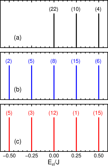
Figure 1: Eigenenergies and their degeneracy (numbers above vertical lines) for a single spin-orbital superexchange bond in $R$VO₃ at $\eta=0$, described by: (a) classical Ising-like interactions (23), (b) Ising-like interactions for $S=1$ spins but full quantum interaction for $\tau=\frac{1}{2}$ pseudospins (24), and (c) the full quantum model (22). Spin-orbital entanglement is absent here, but orbital fluctuations change the energy spectrum in a dramatic way and stabilize the high-spin state.

The full bond Hamiltonian (22) has however also negative eigenvalues and the energy spectrum which includes quantum fluctuations starts at a much lower energy $E_{1}=-\frac{1}{2}J$, see figure 1(c), obtained for a pseudospin singlet ${\tau}_{t}=0$ and the high spin ${\cal S}_{t}=2$ state. The exact spectrum, shown in figure 1(c), is obtained by considering all eigenstates with ${\cal S}=0,1,2$ and $\tau_{o}=0,1$. In fact, it is even sufficient here to consider only the exact values of the ${\vec{\tau}}_{1}\cdot{\vec{\tau}}_{2}$ operator for the orbital singlet ($\tau_{o}=0$) and orbital triplet ($\tau_{o}=1$) states and to keep the Ising form of the spin interaction (23) to reproduce all exact eigenenergies for a single bond, see figure 1(b). However, only when the spin configurations and the eigenstates of total spin ${\cal S}$ are used, the degeneracies of all the states in the spectrum are incorrect, cf. figures 1(b) and 1(c). Therefore, we note that the thermodynamic properties determined in the MF theory are not free from systematic errors. We show below that full spin and orbital dynamics on the bond plays a very important role in systems where orbital correlations contribute by quantum effects.

Yet, there is even a more serious problem which concerns the spin-orbital superexchange (13) — the possible entanglement of spin and orbital operators. Entanglement means here that wave functions cannot be written as products of spin and orbital states, similar to entangled spin singlet wave function [2, 3, 4], where it is not just one eigenstate of the $S^{z}_{i}$ spin operator at site $i$. As the wave functions in the present example obey the SU(2) symmetry in spin and orbital subspace, entanglement does not occur for a single bond, where only individual spin singlet or orbital singlet states are entangled. However, spin-orbital entanglement is a characteristic feature of any spin-orbital model in a larger system, both on a finite cluster and in the thermodynamic limit. There the same spin and orbital operators participate in interactions along several bonds, and we show below that this is also the case for the interaction in equation (22). The essence of this type of entanglement is explained in the following section.

3.2 Entanglement in the SU(2)$\otimes$SU(2) spin-orbital model

Before demonstrating spin-orbital entanglement in more realistic models which apply to systems with active $t_{2g}$ orbital degrees of freedom, we consider first the SU(2)$\otimes$SU(2) spin-orbital model, with $S=\frac{1}{2}$ spins and orbital interactions given by a scalar product $\vec{\tau}_{i}\cdot\vec{\tau}_{j}$ for $\tau=\frac{1}{2}$ pseudospin operators. Two components of $\tau=\frac{1}{2}$ pseudospin stand for two active $t_{2g}$ orbitals along the $\gamma$ axis in a cubic (perovskite) lattice. Indeed, for a given cubic direction only two $t_{2g}$ orbitals are active [66] and the orbital superexchange has SU(2) symmetry when Hund’s exchange is neglected.

Here we shall analyse the energy in the 1D SU(2)$\times$SU(2) model,

$${\cal H}_{J}=J\sum_{i}\Big{(}{\vec{S}}_{i}\cdot{\vec{S}}_{i+1}+x\Big{)}\Big{(}{\vec{\tau}}_{i}\cdot{\vec{\tau}}_{i+1}+y\Big{)}\,,$$ (25)

for spins $S=\frac{1}{2}$ and pseudospins $\tau=\frac{1}{2}$, using exact diagonalization of finite chains with periodic boundary conditions (PBC). The model (25) has two parameters $x$ and $y$. Its phase diagram in the $(x,y)$ plane consists of five distinct phases which result from the competition between effective AF and FM spin, as well as AO and FO pseudospin exchange interactions on the bonds [72]. First of all, the spin and pseudospin correlations are FM/FO, if $x<-{1\over 4}$ and $y<-{1\over 4}$. Then the GS is characterized by the maximal values of both total quantum numbers, ${\cal S}_{t}={\cal T}_{t}=N/2$, where $N$ is the chain length; its degeneracy is $d=(N+1)^{2}$. Two other phases have either FM spin or FO pseudospin order, accompanied by alternating order in the other channel, i.e., AF order for the FO phase and AO order for the FM phase.

A unique feature of FM state is that it is an eigenstate of the Heisenberg exchange operator. The applies to the orbital interactions, so the quantum fluctuations are entirely suppressed in the FM/FO phase. They are also partly suppressed in the FM/AO and AF/FO phases. In all these situations there is no possibility of joint spin-orbital fluctuations as the wave function of the GS is exactly known and has no quantum fluctuations in at least one of the two complementary subspaces. Under these circumstances separation of spin and orbital operators becomes exact and the GS is disentangled. This does not concern excited states [73], but in this section we are interested only in entanglement in the GS. Note, however, that at the special point $x=y=-\frac{1}{4}$ one finds even three degenerate collective excitations: spin, orbital and spin-orbital wave, and the latter excitation is robust and does not decay into separate spin and orbital excitation [74].

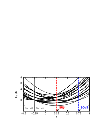
Figure 2: Energy spectrum for the spin-orbital chain (25) of $N=4$ sites with periodic boundaru conditions and $x=y=p$, for increasing $p$. At $p=-\frac{1}{4}$ the GS changes from high spin-orbital state (${\cal S}={\cal T}=2$ with degeneracy $d=25$) to spin-orbital singlet state (${\cal S}={\cal T}=0$ with $d=1$). The point with SU(4) symmetry ($p=\frac{1}{4}$ with $d=1$) and the special SOVB point ($p=\frac{3}{4}$ with $d=2$) are marked by vertical dashed lines. This figure is reproduced from [76].

First we consider the variation of the full energy spectrum of a finite $N=4$ site chain when the FM/FO state changes into the regime dominated by spin and orbital singlets. Therefere we study the SU(2)$\otimes$SU(2) model (25) along the symmetric line in the parameter space, $p=x=y$, see figure 2. Along this line interactions for $S=\frac{1}{2}$ spins and $\tau=\frac{1}{2}$ pseudospins appear on equal footing. At $p=\frac{1}{4}$ one finds the high-symmetry SU(4) point and all three correlation functions are equal: $S_{ij}$ (19) , $T_{ij}$ (20), and ${4\over 3}\langle({\vec{S}}_{i}\cdot{\vec{S}}_{i+1})({\vec{T}}_{i}\cdot{\vec{T}}_{i+1})\rangle$ [75]. On the other hand, at $p=\frac{3}{4}$ the model (25) reads as a product of spin triplet and orbital triplet projection operators at each bond and its GS is exactly solvable — one finds two equivalent states with alternating spin and orbital singlets forming a spin-orbital valence bond (SOVB) phase [76]. These states may be obtained by a similar consideration as the Majumdar-Ghosh valence bond (VB) states in the 1D frustrated $J_{1}-J_{2}$ spin model with nearest $J_{1}$ and next-nearest neighbour $J_{2}$ interactions, at $J_{2}=\frac{1}{2}J_{1}$ [77]. The energy $E_{0}=0$ is given rigorously by alternating spin and orbital singlets along the chain.

One finds a quantum phase transition (QPT) between the high spin-orbital FM/FO state (${\cal S}_{t}={\cal T}_{t}=2$) and the singlet entangled state (${\cal S}_{t}={\cal T}_{t}=0$) in the 1D model (25), see figure 2. The QPT that occurs at $p=-\frac{1}{4}$ is first order, as the energy levels shown in figure 2 cross and all intersite correlations change abruptly, see figure 3(b). At this point the Hamiltonian (25) is a product of spin singlet and orbital singlet projection operators at each bond, so the FM/FO state has the lowest possible energy $E_{0}=0$. But it suffices that either spin or orbital state is a triplet and thus the degeneracy of the GS is here much higher. The role of quantum fluctuations in the regime of $p>\frac{1}{4}$ is easily recognized by considering further variation of the GS energy $E_{0}$ with increasing $p$, see figure 2. Classically the energy of the model (25) would be minimal at $p=0$, but the quantum effects shift the energy minimum to the SU(4) point $p=\frac{1}{4}$; this state is nondegenerate. The energy $E_{0}=0$ is obtained again at $p=\frac{3}{4}$, where the Hamiltonian (25) is a product of spin triplet and orbital triplet projection operators at each bond — here one finds the SOVB phase explained above.

While the GS energy $E_{0}$ per bond of the 1D spin-orbital model (25) is exactly reproduced by the MF energy normalized per one bond $E_{\rm MF}$ in the entire regime of singlet states (${\cal S}_{t}={\cal T}_{t}=0$) for $p<-\frac{1}{4}$,

$$E_{\rm MF}=\Big{(}\Big{\langle}{\vec{S}}_{i}\cdot{\vec{S}}_{i+1}\Big{\rangle}+p\Big{)}\Big{(}\Big{\langle}{\vec{T}}_{i}\cdot{\vec{T}}_{i+1}\Big{\rangle}+p\Big{)},$$ (26)

one finds large corrections to the MF energy for $p>-\frac{1}{4}$, see figure 3(a). This confirms that this MF decoupling procedure is not allowed as joint spin-orbital quantum fluctuations are then ignored which leads to uncontrollable errors in bond correlations.

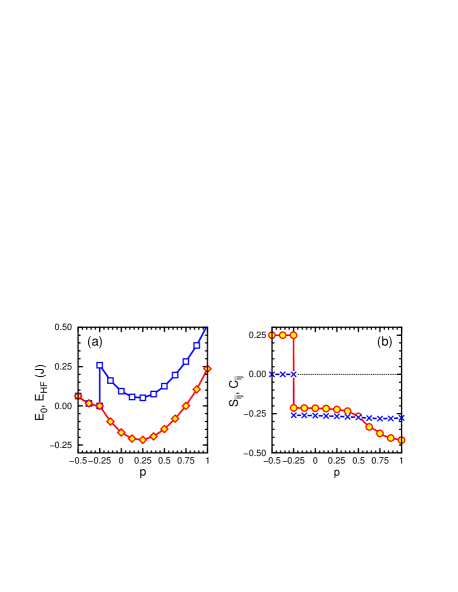
Figure 3: Signatures of entangled spin and orbital operators in the SU(2)$\otimes$SU(2) model (25), obtained by exact diagonalization of the 1D chain of $N=8$ sites at $x=y$ with PBC: (a) the exact GS energy $E_{0}$ (diamonds) and mean field energy $E_{\rm MF}$ (squares) per bond; (b) intersite spin correlations $S_{ij}$ (19) (circles), and composite spin-orbital correlations $C_{ij}$ (21) (crosses); here orbital correlations (20) are degenerate with spin ones, $T_{ij}=S_{ij}$. Entangled GS is found for $p>-0.25$ [76].

To characterize spin-orbital entanglement in the GS we evaluate intersite spin, orbital and joint spin-orbital bond correlations, defined in equations (19)-(21), see figure 3(b). Here we use $s=\frac{1}{2}$ in equations (19) and (21). Note that spin and orbital correlations are intially weaker than the classical ones, i.e., $S_{ij}=T_{ij}>-\frac{1}{4}$, as they are disturbed by the joint spin-orbital correlations $C_{ij}$ (21). The latter are negative in the entire regime of $p>-\frac{1}{4}$ and provide the dominating energy gain in the GS, including the SU(4) symmetric $p=\frac{1}{4}$ and the exactly solvable SOVB $p=\frac{3}{4}$ points. It is of importance that spin-orbital entanglement is related to local properties of spins and orbitals on a bond. Therefore the entanglement phase diagram of a finite system is in agrement with the magnetic and orbital phase diagram of the infinite SU(2)$\otimes$SU(2) model [78].

Another and a more precise quantity to quantify spin-orbital entanglement is von Neumann entropy defined as follows [79],

$${\cal S}_{S\tau}\equiv-\Tr_{S}\{\rho_{S}\,\log_{2}\rho_{S}\}\,,$$ (27)

where $\rho_{S}\equiv\Tr_{\tau}\{|\Psi\rangle\langle\Psi|\}$ is the reduced density matrix of the spin part in the state $|\Psi\rangle$ by integrating out all the orbital degrees of freedom by $\Tr_{\tau}\{\cdots\}$. This measure captures well the correlation between the two types of degrees of freedom, and when spin and orbital operators factorize one finds ${\cal S}_{S\tau}=0$. It has been shown that von Neumann entropy makes a jump at the QPTs between the disentangled and entangled states [79] and may therefore be used to investigate the phase diagram of the SU(2)$\otimes$SU(2) model. We suggest that QPTs in more complex systems of strongly correlated electrons may be investigated by calculating von Neumann entropy in the future.

3.3 Entanglement in $t_{2g}$ spin-orbital models

Entanglement plays an important role in realistic spin-orbital models for $t_{2g}$ orbital degrees of freedom which may be considered as being more quantum than the respective models for $e_{g}$ electrons. This is a consequence of two orbital flavours being active along each cubic axis, while in $e_{g}$ systems there is de facto just one directional orbital which is active along a given cubic axis while the other orbital is inactive, so these latter models are more classical.

The best known example of transition metal oxides with the physical properties controlled by spin-orbital entanglement are the $R$VO₃ perovskites. Two magnetic phases compete with each other at low temperature, and one finds the $C$-AF phase accompanied by $G$-AO order in compounds with a large ionic radius $r_{R}$ of $R$ ions, i.e., for Pr,$\cdots$,La, while for $R$ ions with smaller ionic radius the $G$-AF phase accompanied by $C$-AO order is more stable at $T=0$ and the $C$-AF phase occurs only in a window of finite temperature. In these phases both the magnetic moments and the occupied orbitals alternate in the $ab$ planes along both cubic axes, but the order along the $c$ axis is different, as shown in figure 4. Note that along the $c$ axis the Goodeneough-Kanamori rules are obeyed. The situation looks different for the $ab$ planes, where the magnetic moments and occupied orbitals alternate, see also section 6, but one should keep in mind that inactive $c$ orbitals are singly occupied at every site and rather strong AF superexchange arises along both the $a$ and $b$ axis due to their excitations. Thus, one may classify this case as FO order of $c$ orbitals accompanied by AF order of $S=1$ spins, and once again the Goodeneough-Kanamori rules are followed.

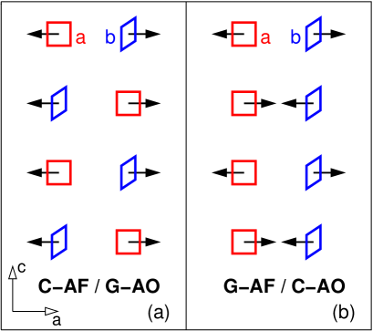
Figure 4: Schematic view of the Goodenough-Kanamori rules on the example of two AF phases observed in the $R$VO₃ perovskites, with complementary magnetic (arrows) and orbital (squares) order of active $t_{2g}$ orbitals $\{a,b\}$ in the $ac$ plane: (a) $C$-AF spin order accompanied by $G$-AF orbital order; (b) $G$-AF spin order accompanied by $C$-AF orbital order. Both spins and orbitals alternate along the $b$ axis (not shown). This figure is reproduced from [11].

Although the above discussion shows that the GS of the $R$VO₃ compounds does not include spin-orbital entanglement, it is of interest to investigate the spin orbital models for the perovskite systems with active $t_{2g}$ orbitals: ($i$) the titanate model ($d^{1}$ model) valid for the $R$TiO₃ perovskites [60, 61], and ($ii$) the vanadate model ($d^{2}$ model) which describes the $R$VO₃ perovskites [67, 71]. Spin-orbital entanglement arises along the $c$ axis, where both active $t_{2g}$ orbitals $\{a,b\}$ contribute and may lead to entangled states. To avoid additional complications due to partly occupied orbitals, one may assume that the $c$ orbitals are empty at every site in the $d^{1}$ model, while they are occupied in the $d^{2}$ model — in both cases they cannot lead to any entangled states.

The spin-orbital models for the cubic perovskites with active $t_{2g}$ orbital degrees of freedom at either Ti³⁺or V³⁺ ions are of the general form given in equation (13). The orbital operators ${\hat{\cal J}}_{ij}^{(\gamma)}$ and ${\hat{\cal K}}_{ij}^{(\gamma)}$ are rather complex and depend on the multiplet structure of the Ti²⁺ and V²⁺ excited states, respectively. They include the terms which break the SU(2) symmetry of the orbital interactions present at $\eta=0$, reducing it to the cubic symmetry. Their explicit form may be found in the original publications. Here we give only the simplified SU(2)$\otimes$SU(2) form of the interactions for the bonds along the $c$ axis,

$${\cal H}_{J}=\frac{1}{2}J\sum_{i}\Big{(}{\vec{S}}_{i}\cdot{\vec{S}}_{i+1}+S^{2}\Big{)}\Big{(}{\vec{\tau}}_{i}\cdot{\vec{\tau}}_{i+1}+\frac{1}{4}\Big{)}\,,$$ (28)

where spin-orbital entanglement is expected. For $S=\frac{1}{2}$ and $S=1$ the above general form reproduces the respective limits obtained for the $d^{1}$ and $d^{2}$ models at $\eta=0$; otherwise it is approximate. We assume below that

$$n_{ia}+n_{ib}=1$$ (29)

for $t_{2g}$ orbitals (8) in case of the $d^{1}$ model, and $n_{ic}=0$.

In the $R$VO₃ perovskites, the crystal-field splitting breaks the cubic symmetry in distorted VO₆ octahedra, as suggested by the electronic structure calculations [80] and derived using the point charge model [81]. One finds again the same filling of $\{a,b\}$ orbitals as given in equation (29), but $n_{ic}=1$. This defines the $t_{2g}$ orbital degrees of freedom in both cases as $\{a,b\}\equiv\{yz,zx\}$ orbitals along every cubic direction, and the superexchange (40) contains the orbital operators ${\vec{\tau}}_{i}=\{\tau_{i}^{+},\tau_{i}^{-},\tau_{i}^{z}\}$ (and their components).

A method of choice to demonstrate spin-orbital entanglement is here again exact diagonalization of finite chains, performed for both the $d^{1}$ and $d^{2}$ model [1]. In the $d^{1}$ model the Hamiltonian at $\eta=0$ reduces to the SU(4) model, and indeed all three bond correlation functions are equal for $N=4$ sites [1], $S_{ij}=T_{ij}=C_{ij}=-0.25$ as shown in figure 5(a). For larger systems these correlations are also equal but somewhat weaker and one finds $S_{ij}=T_{ij}=C_{ij}=-0.21502$ in the thermodynamic limit [75]. By a closer inspection one obtains that the GS wave function for the four-site cluster is close to a total spin-orbital singlet, involving a linear combination of (spin singlet/orbital triplet) and (spin triplet/orbital singlet) states for each bond $\langle ij\rangle$. This result manifestly contradicts the celebrated Goodenough-Kanamori rules [14], as both spin and orbital correlations have the same sign. When $\eta$ increases, the charge fluctuations which contribute to the superexchange concern different states in the multiplet structure breaks the SU(4) symmetry — one finds that the bond correlations are then different and $T_{ij}<C_{ij}<S_{ij}<0$ in the regime of spin singlet (${\cal S}_{t}=0$) GS. Here the Goodenough-Kanamori rule which suggests complementary spin/orbital correlations is still violated.

The vanadate $d^{2}$ model (for $S=1$ spins) [71] behaves also in a similar way in a range of small values of $\eta$, with all three $S_{ij}$, $T_{ij}$ and $C_{ij}$ correlations being negative, see figure 5(b). Most importantly, the composite spin-orbital correlations are here finite ($C_{ij}<0$) which implies that spin and orbital variables are entangled, and the MF factorization of the GS into spin and orbital part fails. In this regime the spin and orbital correlations are both negative and contradict the Goodenough-Kanamori rules [14] of their complementary behaviour. Only for sufficiently large $\eta$ do the spins reorient at the QPT to the FM GS, and decouple from the orbitals. In this regime, corresponding to the experimentally observed $C$-AF phase of LaVO₃ (and other cubic vanadates), spin-orbital entanglement ceases to exist in the GS. However, as we will see below, it has still remarkable consequences in experiments at finite temperature, where entangled spin-orbital excited states contribute and decide about the thermodynamic properties.

A crucial observation concerning the applicability of the Goodenough-Kanamori rules to the quantum models of $t_{2g}$ electrons in one dimension can be made by comparing spin exchange constants $J_{ij}$ calculated from the exact GS $|\Phi\rangle$,

$$J_{ij}=\langle\Phi|{\hat{\cal J}}_{ij}^{(\gamma)}|\Phi\rangle\,,$$ (30)

with intersite spin correlations $S_{ij}$ (19) obtained also exactly. One finds that exchange interaction which is formally FM ($J_{ij}<0$) in the orbital-disordered phase at low values of $\eta$ [see figure 5(c) and figure 5(d)] is in fact accompanied by AF spin correlations ($S_{ij}<0$), so $J_{ij}S_{ij}>0$ and the GS energy calculated in the MF theory is de facto enhanced by this term [1], contrary to what happens in reality.

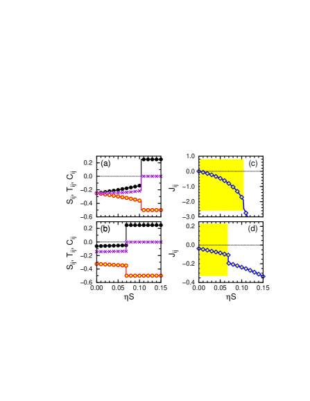
Figure 5: Evolution of: (a-b) intersite spin $S_{ij}$ (19) (filled circles), orbital $T_{ij}$ (20) (empty circles), and spin-orbital $C_{ij}$ (21) ($\times$) correlations, and (c-d) exchange constants $J_{ij}$ (14) along the $c$ axis, obtained by exact diagonalizaton of spin-orbital model on a 1D chain of $N=4$ sites with periodic boundary conditions, for increasing Hund’s exchange $\eta$. Panels (a,c) for $S=1/2$; panels (b,d) for $S=1$. In the shaded areas of (c) and (d) the negative spin correlations $S_{ij}<0$ do not follow the sign of the exchange constant $J_{ij}<0$, and the classical Goodenough-Kanamori rules are violated. This figure is reproduced from [11].

In contrast, similar analysis (not shown) performed for the $d^{9}$ spin-orbital model (13) derived for Cu²⁺ ions with $e_{g}$ orbital degrees of freedom in KCuF₃ [70], gave correctly $J_{ij}S_{ij}<0$. Hence, in spite of enhanced quantum fluctuations of the spin-orbital nature [22], one finds here that spin correlations follow the sign of the exchange constant [1]. This remarkable difference between $t_{2g}$ and $e_{g}$ systems originates from composite spin-orbital fluctuations, which are responsible for the ‘dynamical’ nature of exchange constants in the former case. They exhibit large fluctuations around the average value, measured by the variance,

$$\delta J\equiv\Big{\{}\langle\Phi|({\hat{\cal J}}_{ij}^{(\gamma)})^{2}|\Phi\rangle-J_{ij}^{2}\Big{\}}^{1/2}\,.$$ (31)

Here again the average is calculated exactly from the Lanczos diagonalization of a finite chain of length $N=4$ sites.

As an illustrative example, we give here the values found in the $d^{1}$ and $d^{2}$ model at $\eta=0$ [1]. While the average spin exchange constant is small in both cases ($J_{ij}\simeq 0$ for $d^{1}$, $J_{ij}\simeq-0.04$ for $d^{2}$), $\hat{\cal J}_{ij}^{(\gamma)}$ fluctuates widely over both positive and negative values. In the $d^{1}$ model the fluctuations between ($S=0$/$T=1$) and ($S=1$/$T=0$) wave functions on the bond are so large that $\delta J=1$ ! They survive even quite far from the high-symmetry SU(4) point (at $\eta\simeq 0.1$), and stabilize spin-orbital singlet phase in a broad regime of $\eta$. Also in the $d^{2}$ model the orbital bond correlations change dynamically from singlet to triplet, resulting in $\delta J>|J_{ij}|$, with $\delta J=\frac{1}{4}\{1-(2T_{ij}+\frac{1}{2})^{2}\}^{1/2}\simeq 0.25$, while these fluctuations are small for $d^{9}$ model involving $e_{g}$ orbitals, see also section 5.1.

We emphasize that spin and orbital correlations on the bonds, as well as composite spin-orbital correlations which occur in spin-orbital entangled states for realistic parameters with finite Hund’s exchange, determine the magnetic and optical properties of titanates and vanadates. These correlations change with increasing temperature as then also excited states contribute and decide about their thermal evolution. Therefore, the correct theoretical description of experimental results is challenging and requires adequate treatment of excited states which captures their essential features, including their possible entanglement. This makes simple approaches based on the MF decoupling of spin and orbital operators not reliable and requires either exact diagonalization of finite clusters or advanced numerical methods such as multiscale entanglement renormalization ansatz (MERA) [82].

In the next section we show that composite spin-orbital fluctuations play a crucial role in the $R$VO₃ perovskites. They are responsible for the temperature dependence of the optical spectral weights in LaVO₃ [35], contribute to the remarkable phase diagram of these systems [81] and trigger spin-orbital dimerization in the $C$-AF phase of YVO₃ in the intermediate temperature regime [83]. Remarkably, all these properties including the observed dimerization in the magnetic excitations may be seen as signatures of spin-orbital entanglement in the excited states which becomes relevant at finite temperature.

4 Entangled states in the RVO₃ perovskites

4.1 Optical spectral weights for LaVO₃

The coupling between spin and orbital operators in the spin-orbital superexchange may be so strong in some cases that it leads to a phase transition modifies the magnetic order and excitations at finite temperature — an excellent example of this behaviour are the $R$VO₃ perovskites, as explained below. Although the $C$-AF phase, observed in the entire family of $R$VO₃ compounds [21], where $R$=Lu,$\cdots$,La stands for a rare earth atom, satisfies to some extent the Goodenough–Kanamori rules [14], with FM order along the $c$ axis where the active $a$ and $b$ orbitals (8) alternate — the $G$-AO order of $\{a,b\}$ orbitals is very weak here and the orbital fluctuations play a very important role [67]. This situation is opposite to the frozen and classical AO order in LaMnO₃, which can explain both the observed magnetic exchange constants [13] and the distribution of the optical spectral weights [16]. In LaVO₃ the FM exchange interaction is enhanced far beyond the usual mechanism following from the splitting between the high-spin and low-spin states due to finite Hund’s exchange $J_{H}$. Evidence of orbital fluctuations in the $R$VO₃ perovskites was also found in pressure experiments, which show a distinct competition between the $C$-AF and $G$-AF spin order, accompanied by the complementary $G$-AO and $C$-AO order of $\{a,b\}$ orbitals [21].

The spin and orbital order along the $c$ axis are not entangled in the GS of the $R$VO₃ perovskites (due to either FM or FO order), but entangled states contribute at finite temperature. As the first manifestation of spin-orbital entanglement in the cubic vanadates at finite temperature we discuss briefly the evaluation of the low-energy optical spectral weight from the spin-orbital superexchange for LaVO₃, following equation (18). The superexchange operator ${\cal H}_{J}$ (17) is here considered for a bond $\langle ij\rangle\parallel\gamma$, and arises as a superposition of individual $d_{i}^{2}d_{j}^{2}\rightleftharpoons d_{i}^{3}d_{j}^{1}$ charge excitations to different spin states in the upper Hubbard subbands labeled by $n$ [35]. One finds the superexchange terms $H^{(c)}_{n,ij}$ for a bond ${\langle ij\rangle}$ along the $c$ axis,

$$H_{n,ij}^{(c)} = -\frac{1}{3}Jr_{1}\left(2\!+\!\vec{S}_{i}\!\cdot\!\vec{S}_{j}\right)\left(\frac{1}{4}-\vec{\tau}_{i}\cdot\vec{\tau}_{j}\right),$$ (32)

$$H_{n,ij}^{(c)} = -\frac{1}{12}J\left(1-\vec{S}_{i}\!\cdot\!\vec{S}_{j}\right)\left(\frac{7}{4}-\!\tau_{i}^{z}\tau_{j}^{z}\!-\!\tau_{i}^{x}\tau_{j}^{x}\!+\!5\tau_{i}^{y}\tau_{j}^{y}\right),$$ (33)

$$H_{n,ij}^{(c)} = -\frac{1}{4}Jr_{3}\left(1-\!\vec{S}_{i}\!\cdot\!\vec{S}_{j}\right)\left(\frac{1}{4}+\tau_{i}^{z}\tau_{j}^{z}\!+\tau_{i}^{x}\tau_{j}^{x}-\tau_{i}^{y}\tau_{j}^{y}\!\right),$$ (34)

and $H^{(ab)}_{n,ij}$ for a bond in the $ab$ plane,

$$H_{n,ij}^{(ab)} = -\frac{1}{6}Jr_{1}\!\left(2+\vec{S}_{i}\!\cdot\!\vec{S}_{j}\right)\left(\frac{1}{4}-\tau_{i}^{z}\tau_{j}^{z}\right),$$ (35)

$$H_{n,ij}^{(ab)} = -\frac{1}{16}J\left(1-\vec{S}_{i}\!\cdot\!\vec{S}_{j}\right)\left(\frac{19}{6}\mp\tau_{i}^{z}\mp\tau_{j}^{z}-\frac{2}{3}\tau_{i}^{z}\tau_{j}^{z}\right),$$ (36)

$$H_{n,ij}^{(ab)} = -\frac{1}{16}Jr_{3}\left(1-\vec{S}_{i}\!\cdot\!\vec{S}_{j}\right)\left(\frac{5}{2}\mp\tau_{i}^{z}\mp\tau_{j}^{z}+2\tau_{i}^{z}\tau_{j}^{z}\right).$$ (37)

When the spectral weight is evaluated following equation (18), it is reasonable to try first the MF approximation and to separate spin and orbital correlations from each other. The spectral weights require then the knowledge of spin correlations $S_{ij}$ (19): along the $c$ axis in (32)-(34), and within the $ab$ planes in (35)-(37), as well as the corresponding intersite orbital correlations $\langle\vec{\tau}_{i}\cdot\vec{\tau}_{j}\rangle$ and $\langle{\tau}_{i}^{\alpha}{\tau}_{j}^{\alpha}\rangle$, with $\alpha=x,y,z$. From the form of the above superexchange contributions one sees that high-spin excitations $H^{(\gamma)}_{n,ij}$ support the FM coupling while the low spin ones, $H^{(\gamma)}_{2,ij}$ and $H^{(\gamma)}_{3,ij}$, contribute with AF couplings. The high-spin spectral weight (18) in the MF approximation is given by

$$w_{c1}^{\rm MF}=\frac{2}{3}Jr_{1}\Big{\langle}\vec{S}_{i}\!\cdot\!\vec{S}_{j}+2\Big{\rangle}\left\langle\frac{1}{4}-\vec{\tau}_{i}\cdot\vec{\tau}_{j}\right\rangle\,.$$ (38)

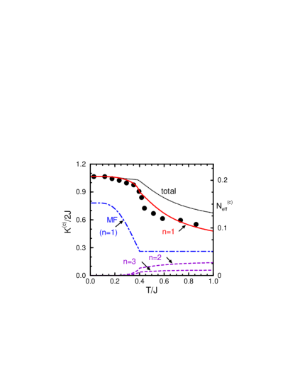
Figure 6: Optical spectral weights $K_{n}^{(c)}$ (18) for the high-spin optical subband ($n=1$; solid line), low-spin optical subbands ($n=2,3$; dashed lines) and total $K^{(c)}$ (dotted line) obtained from the excitations to different Hubbard subbands along the $c$ axis (32)-(34). Filled circles show the effective carrier number $N_{\rm eff}^{(c)}$ (in the energy range $\omega<3$ eV which corresponds to the high-spin excitations) for LaVO₃, presented in Fig. 5 of [25]. Dashed-dotted line shows the spectral weight $K_{1}^{(c)}$ obtained from the MF decoupling (38). Parameters: $\eta=0.12$, $V_{c}=0.9J$, $V_{ab}=0.2J$.

The low-energy optical spectral weight for the polarization along the $c$ axis $K_{\rm 1,exp}^{(c)}$ decreases by a factor close to two when the temperature increases from $T\simeq 0$ to $T=300$ K [25] — this change is much larger than the one observed in LaMnO₃ [16]. However, the theory based on the MF decoupling of the spin and orbital degrees of freedom gives only a much smaller reduction of the weight close to 33% when a frozen orbital order (similar to LaMnO₃) with $\langle\vec{\tau}_{i}\cdot\vec{\tau}_{j}\rangle=-\frac{1}{4}$ is assumed and has to fail in explaining the experimental data [13]. In spite of weakening spin and orbital intersite correlations when the temperature increases in the experimental range $0<T<300$ K, this variation is clearly not sufficient to describe the experimental data. Instead, when both spin and orbital correlations are reduced and vanish above the common transition temperature $T_{\rm N1}=T_{\rm OO}$, the MF theory predicts that the spectral weight decrease fast and do not change above $T_{\rm N1}$, see figure 6, contrary to experiment.

On the other hand, when a cluster method is used to determine the optical spectral weight from the high-spin superexchange term (32) by including orbital as well as joint spin-and-orbital fluctuations along the $c$ axis, the temperature dependence of the spectral weight resulting from the theory persists above $T_{\rm N1}$ and follows the experimental data [35], see figure 6. In this approach a cluster of $N=4$ sites is solved exactly with the MFs originating from the spin and orbital order below $T_{\rm N1}$ and $T_{\rm OO}$, respectively, and a free cluster is solved at high temperature when the long-range order vanishes. This reflects the realistic temperature dependence with spin and orbital correlations being finite in this latter regime, in contrast to the one-site MF approach.

The satisfactory description of the experimental data shown in figure 6 may be considered as a remarkable success of the theory based on the spin-orbital superexchange model derived for the $R$VO₃ perovskites. It proves that spin-orbital entangled states contribute in a crucial way in the entire regime of finite temperature. In addition, the theoretical calculation predicts that the high energy spectral weight ($n=2,3$) is low for the polarization along the $c$ axis. The spectral weight in the $ab$ planes behaves in the opposite way — it is small at low energy, and large at high energy (but not as large as the low-energy one for the $c$ axis). This weight distribution and its anisotropy between the $c$ and $ab$ directions reflects the nature of spin correlations on the bonds, which are FM and AF in these two directions. We expect that future experiments will confirm these theory predictions for the $ab$ polarization.

4.2 Phase diagram of the $R$VO₃ perovskites

The phase diagram of the $R$MnO₃ perovskites [84] indicates that spin and orbital energy scales separate which makes it possible to describe the experimental data for the magnetic exchange constants and the optical spectral weights using the disentangled spin-orbital superexchange [13, 16]. In contrast, in the $R$VO₃ perovskites the phase diagram suggests the proximity of spin and orbital energy scales [21]. Experimental studies have shown that the $C$-AF order is common to the entire family of the $R$VO₃ vanadates, and in general the magnetic transition occurs soon below the orbital transition when the temperature is lowered further, i.e., $T_{\rm N1}<T_{\rm OO}$. LaVO₃ is an exception here and these transitions occur almost simultaneously, with $T_{\rm N1}\simeq T_{\rm OO}$ [21].

When the ionic radius $r_{R}$ decreases, the Néel temperature $T_{\rm N1}$ also decreases, while the orbital transition temperature $T_{\rm OO}$ increases, passes through a maximum close to YVO₃, and next decreases when LuVO₃ is approached [21]. One finds that the $C$-AF order develops in LaVO₃ below $T_{N1}\simeq 143$ K, and is almost immediately followed by a weak structural transition stabilizing the weak $G$-AO order at $T_{\rm OO}\simeq 141$ K [21]. This provides a constraint on the theoretical model and is an experimental challenge to the theory which was addressed using the spin-orbital superexchange model extended by the orbital-lattice coupling [81].

In order to unravel the physical mechanism responsible for the surprising decrease of $T_{\rm OO}$ from YVO₃ to LuVO₃ one has to analyse in more detail the evolution of GdFeO₃ distortions for decreasing ionic radius $r_{R}$ [81]. Such distortions are common for the perovskites [85], and one expects that they should increase when the ionic radius $r_{R}$ decreases, as observed in the $R$MnO₃ perovskites [84]. In the $R$VO₃ family the distortions are described by two subsequent rotations of VO₆ octahedra: ($i$) by an angle $\vartheta$ around the $b$ axis, and ($ii$) by an angle $\varphi$ around the $c$ axis. Increasing angle $\vartheta$ causes a decrease of V–O–V bond angle along the $c$ direction, being $\pi-2\vartheta$, and leads to an orthorhombic lattice distortion $u=(b-a)/a$, where $a$ and $b$ are the lattice parameters of the $Pbnm$ structure of $R$VO₃. By the analysis of the structural data for the $R$VO₃ perovskites [86, 87] one finds the following empirical relation between the ionic radius $r_{R}$ and the angle $\vartheta$:

$$r_{R}=r_{0}-\alpha\sin^{2}\vartheta\,,$$ (39)

where $r_{0}=1.5$ Å and $\alpha=0.95$ Å are the empirical parameters. This allows one to use the angle $\vartheta$ to parametrize the dependence of the microscopic parameters of the Hamiltonian and to investigate the transition temperatures $T_{\rm OO}$ and $T_{\rm N1}$ as functions of the ionic radius $r_{R}$.

The spin-orbital model introduced in [81] to describe the phase diagram of $R$VO₃ was thus extended with respect to its original form [67] and reads:

$${\cal H}\! = J\sum_{\langle ij\rangle\parallel\gamma}\left\{\Big{(}{\cal J}_{ij}^{(\gamma)}{\vec{S}}_{i}\!\cdot\!{\vec{S}}_{j}+S^{2}\Big{)}+{{\cal K}}_{ij}^{(\gamma)}\right\}+E_{z}(\vartheta)\!\sum_{i}\!e^{i{\vec{R}}_{i}{\vec{Q}}}\tau_{i}^{z}$$ (40)

$$- V_{c}(\vartheta)\sum_{\langle ij\rangle\parallel c}\tau_{i}^{z}\tau_{j}^{z}+V_{ab}(\vartheta)\sum_{\langle ij\rangle\parallel ab}\tau_{i}^{z}\tau_{j}^{z}$$

$$- gu\sum_{i}\tau_{i}^{x}+\frac{1}{2}NK\{u-u_{0}(\vartheta)\}^{2}\,,$$

where $\gamma=a,b,c$ labels the cubic axes, and the orbital operators ${\cal J}_{ij}^{(\gamma)}$ and ${\cal K}_{ij}^{(\gamma)}$ are given in [71]. The superexchange $\propto J$ is supplemented by the crystal field term $\propto E_{z}$, the orbital interaction terms $\propto V_{c}$ and $\propto V_{ab}$ induced by lattice distortions, and the orbital-lattice term $\propto g$ which is counteracted by the lattice elastic energy $\propto K$. All these terms are necessary in a realistic model [81] to reproduce the complex dependence of the orbital and magnetic transition temperature on the ionic size in the $R$VO₃ perovskites.

The crystal-field splitting $\propto E_{z}$ between $a$ and $b$ orbital energies in equation (40) is given by the pseudospin $\tau_{i}^{z}$ operators,

$$\tau_{i}^{z}=\frac{1}{2}(n_{ia}-n_{ib})\,,$$ (41)

which refer to two active orbital flavors $\{a,b\}$ in $R$VO₃. It is characterized by the vector ${\vec{Q}}=(\pi,\pi,0)$ in reciprocal space and favours the $C$-AO order. Thus, this splitting competes with the (weak) $G$-AO order supporting the observed $C$-AF phase at temperature $T<T_{\rm N1}$, effectively weakening this type of magnetic order.

As for instance in LaMnO₃, the orbital order in the $R$VO₃ perovskites arises due to joint orbital interactions which are a superposition of the superexchange and interactions induced by lattice distortions. These latter terms are twofold: ($i$) intersite orbital interactions $\{V_{ab},V_{c}\}$ (which originate from the coupling to the lattice), and ($ii$) orbital-lattice coupling $\propto g$ which induces orbital polarization $\langle\tau_{i}^{x}\rangle\neq 0$ for finite lattice distortion $u$. The orbital interactions induced by the distortions of the VO₆ octahedra and by the GdFeO₃ distortions of the lattice, $V_{ab}>0$ and $V_{c}>0$, also favour the $C$-AO order (like the crystal field term with $E_{z}>0$). Note that $V_{c}>0$ counteracts the orbital interactions included in the superexchange via ${\hat{K}}_{ij}^{(c)}$ operators.

The last two terms in equation (40) are particularly important for ions with small ionic radii $r_{R}$. They describe the linear coupling $\propto g>0$ between active $\{a,b\}$ orbitals and the orthorhombic lattice distortion $u$. The elastic energy which counteracts lattice distortion $u$ is given by the force constant $K$, and $N$ is the number of $V^{3+}$ ions. The coupling

$$g_{\rm eff}\equiv gu$$ (42)

may be seen as a transverse field in the pseudospin space which competes with the Jahn-Teller terms $\{V_{ab},V_{c}\}$. While the eigenstates of $\tau_{i}^{x}$ operator, $\frac{1}{\sqrt{2}}(|a\rangle\pm|b\rangle)$, cannot be realized due to the competition with all the other terms, increasing lattice distortion $u$ (increasing angle $\vartheta$) gradually modifies the orbital order and intersite orbital correlations towards this type order.

Except for the superexchange parameter $J$, all the parameters in the extended spin-orbital model (40) depend on the tilting angle $\vartheta$. In case of $V_{c}$ one may argue that its dependence on the angle $\vartheta$ is weak, and a constant $V_{c}(\vartheta)\equiv 0.26J$ was chosen in [81] in order to satisfy the experimental constraint that the magnetic and orbital order appear almost simultaneously in LaVO₃ [21]. The experimental value $T_{\rm N1}^{\rm exp}=143$ K for LaVO₃ [21] was fairly well reproduced in the present model taking $J=200$ K, the value which is also consistent with the magnon energy scale [26]. The functional dependence of the remaining two parameters $\{E_{z}(\vartheta),V_{ab}(\vartheta)\}$ on the tilting angle $\vartheta$ was derived from the point charge model [81] using the structural data for the $R$VO₃ series [86, 87] — one finds:

$$E_{z}(\vartheta) = J\,v_{z}\,\sin^{3}\vartheta\cos\vartheta\,,$$ (43)

$$V_{ab}(\vartheta) = J\,v_{ab}\,\sin^{3}\vartheta\cos\vartheta\,.$$ (44)

Finally, the effective coupling to the lattice distortion $g_{\rm eff}(\vartheta)$ (42) has to increase faster with the ncreasing angle $\vartheta$ as otherwise the nonmonotonous dependence of $T_{\rm OO}$ on $\vartheta$ (or on the ionic radius $r_{R}$) cannot be reproduced by the model, and the following dependence was shown [81] to give a satisfactory description of the phase diagram of the $R$VO₃ perovskites:

$$g_{\rm eff}(\vartheta)=J\,v_{g}\,\sin^{5}\vartheta\cos\vartheta\,.$$ (45)

Altogether, magnetic and orbital correlations described by the spin-orbital model (40), and the magnetic $T_{\rm N1}$ and orbital $T_{\rm OO}$ transition temperatures, depend on three parameters: $\{v_{z},v_{ab},v_{g}\}$.

Due to the spin-orbital entanglement which is activated by finite temperature in the $R$VO₃ perovskites, it is crucial to design the MF approach in such a way that the spin-orbital coupling is described beyond the factorization of spin and orbital operators. As usually, the correct MF treatment of the orbital and magnetic phase transitions in the $R$VO₃ perovskites requires the coupling between the on-site orbital, $\langle\tau^{z}\rangle_{G}\equiv\frac{1}{2}|\langle\tau^{z}_{i}-\tau^{z}_{j}\rangle|$, and spin order parameters in the $C$-AF phase, $\langle S_{i}^{z}\rangle_{C}$, as well as including a composite spin-orbital $\langle S_{i}^{z}\tau_{i}^{z}\rangle$ order parameter, similar to that introduced before for the $R$MnO₃ perovskites [12]. However, the on-site MF approach including the above coupling [88] does not suffice for the $R$VO₃ compounds as the orbital singlet correlations $\langle{\vec{\tau}}_{i}\cdot{\vec{\tau}}_{j}\rangle$ on the bonds along the $c$ axis play here a crucial role in stabilizing the $C$-AF phase [67] and the orbital fluctuations are also important [89]. Therefore, the minimal physically acceptable approach to the present problem is a self-consistent calculation od spin and orbital correlations for an embedded bond $\langle ij\rangle$ along the $c$ axis, coupled by the MF terms to its neighbours along all three cubic axes [81]. This procedure, with properly selected model parameters, led to the successful description of the experimental phase diagram [21], see figure 7. The evolution of the orbital correlations with varying temperature and with decreasing $r_{R}$ plays a prominent role in the success of the theoretical description of the phase diagram of the $R$VO₃ perovskites. One finds that indeed the orbital order occurs first at a higher temperature and is followed by the magnetic transition in the $R$VO₃ perovskites with a smaller ionic radius $r_{R}$, to the left of LaVO₃.

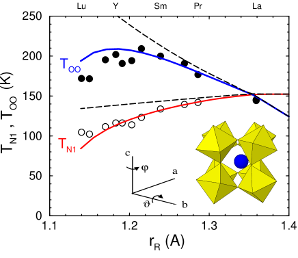
Figure 7: The orbital transition temperature $T_{\rm OO}$ and Néel transition temperature $T_{\rm N1}$ for the onset $C$-AF order as functions of varying ionic size $r_{R}$ in the $R$VO₃ perovskites, as obtained in experiment (full and empty circles) and from the theory (solid lines). Dashed lines show $T_{\rm OO}$ and $T_{\rm N1}$ obtained under neglect of orbital-lattice coupling (at $g=0$). The inset shows the GdFeO₃-type distortion, with the rotation angles $\vartheta$ and $\varphi$ corresponding to the data of YVO₃ [86]. This figure is reproduced from [81].

The non-monotonous dependence of the orbital transition temperature $T_{\rm OO}$ on the ionic radius $r_{R}$ may be understood as follows. $T_{\rm OO}$ increases first with decreasing ionic radius $r_{R}$ as the Jahn-Teller term in the $ab$ planes, $V_{ab}(\vartheta)$, increases and induces the orbital correlations which stabilize the $G$-AO order. The coupling $g_{\rm eff}(\vartheta)$ to the lattice (45) is then rather weak, with $\langle\tau^{x}_{i}\rangle\simeq 0.03$ in LaVO₃, but $g_{\rm eff}$ increases faster than the interaction $V_{ab}(\vartheta)$ (44). Finally, the former term dominates and the $G$-AO order parameter is almost equal to the competing with it ”transverse” moments, $\langle\tau^{x}_{i}\rangle\simeq\langle\tau^{z}_{i}\rangle_{G}$. Therefore, the $G$-AO order gets weaker and the transition temperature $T_{\rm OO}$ is reduced. Note that in the entire parameter range the orbital order parameter $\langle\tau^{x}_{i}\rangle\simeq\langle\tau^{z}_{i}\rangle_{G}$ is substantially reduced from the classical value $\langle\tau^{z}\rangle_{G,\rm max}=\frac{1}{2}$ by singlet orbital fluctuations, being for instance $\langle\tau^{z}_{i}\rangle_{G}\simeq 0.32$ and 0.36 for LaVO₃ and LuVO₃.

It is quite remarkable that the magnetic exchange constants $\{J_{ab},J_{c}\}$ are modified solely by the changes in the orbital correlations described above. The superexchange constant $J$ does not change and the reductions of $T_{\rm N1}$ with decreasing $r_{R}$ follows only from the evolution of the orbital state [81]. One finds that also the width of the magnon band, given by$W_{C-{\rm AF}}=4(J_{ab}+|J_{c}|)$ at $T=0$, is reduced by a factor close to 1.8 from LaVO₃ to YVO₃. This also agrees qualitatively with surprisingly low magnon energies observed in the $C$-AF phase of YVO₃ [26].

Summarizing, the microscopic model (40) is remarkably successful in describing gradual changes of the orbital and magnetic correlations under increasing Jahn-Teller interactions and the coupling to the lattice which both suppress the orbital fluctuations along the $c$ axis, responsible for rather strong FM spin-orbital superexchange [67]. It describes well the systematic experimental trends for both orbital and magnetic transitions in the $R$VO₃ perovskites [81], and is able to reproduce the observed non-monotonic variation of the orbital transition temperature $T_{\rm OO}$ for decreasing ionic radius $r_{R}$. Another consequence of the spin-orbital entanglement in the perovskite vanadates, the spin-orbital dimerization along the $c$ axis in YVO₃, is shortly discussed in the next subsection.

4.3 Peierls dimerization in YVO₃

The third and final example of the spin-orbital entanglement at finite temperature in the family of vanadate perovskites is the existence of a remarkable first order magnetic transition at $T_{\rm N2}=77$ K from the $G$-AF to the $C$-AF spin order with rather exotic magnetic properties, found in YVO₃ [90]. This magnetic transition is surprising and rather unusual as the staggered moments are approximately parallel to the $c$ axis in the $G$-AF phase, and reorient above $T_{\rm N2}$ to the $ab$ planes in the $C$-AF phase, with some small alternating $G$-AF component along the $c$ axis. First, while the orientations of spins in $C$-AF and $G$-AF phase are consistent with the expected anisotropy due to spin-orbit coupling [83], the observed magnetization reversal with the weak FM component remains puzzling and found no explanation in the theory so far. Second, it was also established by neutron scattering experiments [26] that the energy scale of magnetic excitations is considerably reduced for the $C$–AF phase (by a factor close to two) as compared with the magnon dispersion measured in the $G$-AF phase. The magnetic order parameter in the $C$-AF phase of LaVO₃ is also strongly reduced to $\simeq 1.3\mu_{B}$, which cannot be explained by rather small quantum fluctuations in the $C$-AF phase [91]. Finally, the $C$-AF phase of YVO₃ is dimerized. Until now, only this last feature found a satisfactory explanation in the theory [92], see below.

The observed dimerization in the magnon spectra in YVO₃ motivated the search for its mechanism within the spin-orbital superexchange model. Dimerization of AF spin chains coupled to phonons is well known and occurs in several systems [93]. In the spin-orbital model for the $R$VO₃ perovskites a similar instability might also occur without the coupling to the lattice when Hund’s exchange is sufficiently small. In particular, the GS at $\eta=0$ may be approximated by the dimerized chain with strong FM bonds alternating with the AF ones, if such chains are coupled by AF interactions along the $a$ and $b$ axes [94] (the 1D chain would give then the entangled disordered GS). For finite and realistic $\eta\simeq 0.13$ the chain is FM (due to the weak coupling to the neighbouring chains in $ab$ planes) [71] and at first instance any dimerization appears surprising.

Before addressing the question of magnon excitations in the $C$-AF phase of YVO₃ stable at intermediate temperature, let us consider first the 1D spin-orbital superexchange model along the $c$ axis, as in YVO₃. The Hamiltonian is given by [92],

$$H_{S\tau}=J\sum_{j}\left(\vec{S}_{j}\!\cdot\!\vec{S}_{j+1}+1\right)\left(\vec{\tau}_{j}\!\cdot\!\vec{\tau}_{j+1}+\frac{1}{4}-\gamma_{H}\right),$$ (46)

where $\vec{S}_{j}$ represent $S=1$ spins and $\vec{\tau}_{j}$ are $\tau=\frac{1}{2}$ orbital pseudospins, respectively, and $\gamma_{H}$ is a constant proportional to Hund’s exchange which stabilizes FM spin correlations. This expression is somewhat simplified with respect to the full spin-orbital model for YVO₃ [71], but reflects its essential features and guarantees that the GS is FM when $\gamma_{H}\simeq 0.1$. The FM GS state is disentangled — it is allowed to use the MF decoupling [1], and to decompose the above Hamiltonian (46) into the spin ($H_{S}$) and orbital ($H_{\tau}$) part, $H_{S\tau}\simeq H_{S}+H_{\tau}$. This disentangled chain may be now studied either by density-matrix renormalization group applied to transfer matrices (TMRG) [95], or by an analytical approach, the so-called modified spin-wave theory of Takahashi [96].

It is easy to understand why the spin-orbital dimerization occurs at finite temperature. The crucial concept is the interrelation between spin and orbital correlations in the 1D spin-orbital chain: spin correlations determine the exchange interactions in the orbital channel $H_{\tau}$, and the orbital ones are responsible for the spin exchange in $H_{S}$. In the GS the spin state is rigid, and spin correlations on the bonds $\langle j,j+1\rangle$ along the $c$ axis are saturated, i.e., $\langle{\vec{S}}_{j}\cdot{\vec{S}}_{j+1}\rangle=1$, and do not allow for any alternation in the orbital interactions which are determined by them. But when temperature increases the thermal fluctuations soften the FM order and the spin-orbital chain may dimerise [92]. Important here is the rather dense spectrum of low energy excited states in the spin-orbital chain [97], which are entangled and all contribute to the thermal averages used to calculate spin and orbital correlations. We emphasize that the dimerization in the spin-orbital chain may be seen as a signature of entanglement in excited states in the $C$-AF phase which contribute at finite temperature. The exchange constants alternate along the $c$ direction between a stronger (${\cal J}_{c}^{(1)}$) and weaker (${\cal J}_{c}^{(1)}$) exchange with $\delta_{S}>0$,

$${\cal J}_{c}^{(1)}\equiv{\cal J}_{c}(1+\delta_{S})\,,\hskip 14.22636pt{\cal J}_{c}^{(2)}\equiv{\cal J}_{c}(1-\delta_{S})\,.$$ (47)

Similar expressions are also found for the orbital exchange interactions which favour AO order and have alternating strength with $\delta_{\tau}>0$,

$${\cal J}_{\tau}^{(1)}\equiv{\cal J}_{\tau}(1+\delta_{\tau})\,,\hskip 14.22636pt{\cal J}_{\tau}^{(2)}\equiv{\cal J}_{\tau}(1-\delta_{\tau})\,.$$ (48)

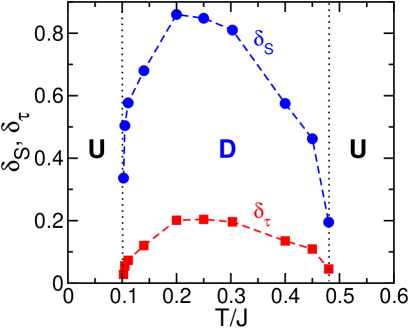
Figure 8: (Color online) Phase diagram with two undimerized (U) phases and a dimerized (D) phase in between, and dimerization parameters $\delta_{S}$ and $\delta_{\tau}$, obtained for the spin-orbital model (46) in the MF decoupling. Dotted vertical lines indicate the onset of a dimerised phase under increasing/decreasing temperature. For more details see [92], where these data were presented and discussed.

While the spin and orbital operators are disentangled in the FM ground state, one may consider a coupled FM spin chain to an orbital chain with interactions which favour weak AO order accompanied by orbital fluctuations, as realized in the $C$-AF phase. The spin (orbital) exchange interaction along the chain is then determined by the bond orbital (spin) correlations. They are defined as follows:

$${\cal J}_{c} \equiv \frac{1}{2}\Big{\langle}\vec{\tau}_{j}\!\cdot\!\vec{\tau}_{j+1}+\vec{\tau}_{j}\!\cdot\!\vec{\tau}_{j-1}\Big{\rangle}+\frac{1}{4}-\gamma_{H}\,,$$ (49)

$${\cal J}_{\tau} \equiv \frac{1}{2}\Big{\langle}\vec{S}_{j}\!\cdot\!\vec{S}_{j+1}+\vec{S}_{j}\!\cdot\!\vec{S}_{j-1}\Big{\rangle}+1\,,$$ (50)

and have to be determined self-consistently, together with spin and orbital correlations along the chain. For the parameters selected in equation (46), one finds that FM spin correlations with ${\cal J}_{c}<0$ are accompanied by ${\cal J}_{\tau}>0$ that favours AO order along the chain. Such complementary spin and orbital correlations are indeed found in the entire temperature regime, in agreement with the Goodenough-Kanamori rules. But in the intermediate temperature range, when the spins start to fluctuate and their correlations are not rigid anymore, the dimerization sets in, see figure 8. Finite temperature is here essential as dimerized spin correlations support then the dimerized orbital correlations. Hence, the dimerization occurs here simultaneously in both channels and has a dome-shaped form, with a maximum at $T\simeq 0.2J$ [92]. The dimerization in the FM chain is much stronger than the one in the AO chain, but they have to coexist in the present self-consistent treatment of this phenomenon. When temperature is high enough, in the present case for $T>0.49J$, the dimerization vanishes again as the spins and the orbitals are disordered by thermal fluctuations. The phase transition at finite temperature between a uniform and a dimerised phase, shown in figure 8, is a consequence of the MF decoupling.

The microscopic model (46), which explains the anisotropy in the exchange constants (47) as following from the joint dimerization that occurs in the spin-orbital chain with FM spin order at finite temperature [92], helps to understand the magnon dispersion found in YVO₃ by the neutron scattering [26]. The observed spin-wave dispersion may be explained by the following effective spin Hamiltonian for the $C$-AF phase, derived assuming again that the spin and orbital operators may be disentangled which is strictly valid only at $T=0$:

$${\cal H}_{S} = J_{c}\sum_{\langle i,i+1\rangle\parallel c}\left\{1+(-1)^{i}\delta_{S}\right\}{\vec{S}}_{i}\cdot{\vec{S}}_{i+1}$$ (51)

$$+ J_{ab}\sum_{\langle ij\rangle\parallel ab}{\vec{S}}_{i}\cdot{\vec{S}}_{j}+K_{z}\sum_{i}\left(S_{i}^{z}\right)^{2}\,.$$

Following the linear spin-wave (LSW) theory the magnon dispersion is given by

$$\omega_{\pm}({\bf k})=2\sqrt{\left(2J_{ab}+|J_{c}|+\frac{1}{2}K_{z}\pm J_{c}\;\eta_{\bf k}^{1/2}\right)^{2}-\big{(}2J_{ab}\gamma_{\bf k}\big{)}^{2}},$$ (52)

with

$$\gamma_{\bf k} = \frac{1}{2}\left(\cos k_{x}+\cos k_{y}\right)\;,$$ (53)

$$\eta_{\bf k} = \cos^{2}k_{z}+\delta_{S}^{2}\sin^{2}k_{z}\,.$$ (54)

The single-ion anisotropy term $\propto K_{z}$ is responsible for the gap which opens in spin excitations. Two modes measured by the neutron scattering [26] are well reproduced by $\omega_{\pm}({\bf k})$ given by equation (52) when the experimental exchange constants are inserted: $J_{ab}=2.6$ meV, $J_{c}=-3.1$ meV, $\delta_{S}=0.35$, see figure 9 (further improvement including a finite gap at the $\Gamma$ point are obtained taking finite $K_{z}>0$ [26]. This shows that while the essential features seen in the experiment are well reproduced already by the present simplified spin exchange model ${\cal H}_{S}$ (51), the spin interactions are more complex in reality [26].

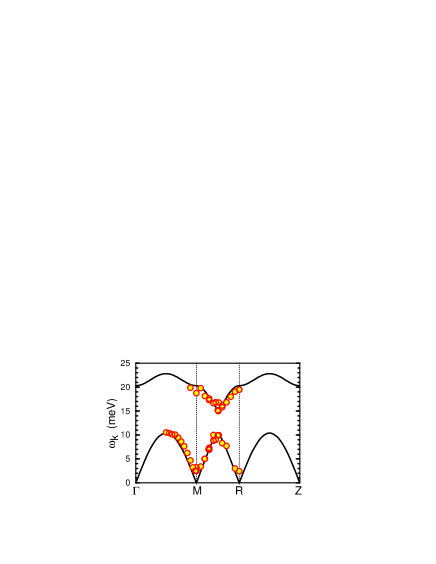
Figure 9: (Color online) Spin-wave dispersions $\omega_{\bf k}$ (solid lines) as obtained in the LSW theory along the representative directions in the Brillouin zone for the dimerized $C$-AF phase of YVO₃ with experimental exchange constants [26]: $J_{ab}=2.6$ meV, $J_{c}=3.1(1\pm\delta_{S})$ meV and $\delta_{S}=0.35$. Parameters: $J=30$ meV, $\eta=0.13$, $\delta_{S}=0.35$, $K_{z}=0$. The experimental points [26] measured by neutron scattering at $T=85$ K are reproduced by circles. The high symmetry points are: $\Gamma=(0,0,0)$, $M=(\pi,\pi,0)$, $R=(\pi,\pi,\pi)$, $Z=(0,0,\pi)$. This figure is reproduced from [71].

Summarizing, spin-orbital entanglement in the excited states is also responsible for the exotic magnetic properties of the $C$-AF phase of YVO₃. They arise from the coupling between the spin and orbital operators which triggers the dimerization of the FM interactions (47) as a manifestation of a universal instability which occurs in FM spin chains at finite temperature, either by the coupling to the lattice or to purely electronic degrees of freedom [92]. This latter mechanism could play a role in many transition metal oxides with (nearly) degenerate orbital states.

5 Entanglement in the ground states of spin-orbital models

5.1 Kugel-Khomskii model

As shown in section 3, the GSs of certain spin-orbital models are entangled and this will likely influence future experimental studies. As an example we discuss here the Kugel-Khomskii $d^{9}$ model on a bilayer and analyse the $d^{1}$ spin-orbital on a frustrated triangular lattice in section 5.2. While the coexistence the $A$-type AF ($A$-AF) order and the $C$-AO order below $T_{\rm N}\simeq 39$ K is well established in the KCuF₃ perovskite [98, 99] and this phase is well reproduced by the spin-orbital superexchange $d^{9}$ model [70], the model poses an interesting theoretical question: which types of coexisting spin-orbital order (or disorder) are possible when its microscopic parameters are varied? So far, it was only established that the long-range AF order is destroyed by strong quantum fluctuations [23, 24, 70], and it has been shown that certain spin disordered phases with VB correlations may be stabilized by local orbital correlations [22, 100]. However, the phase diagram of the Kugel-Khomskii $d^{9}$ model was not studied systematically beyond the MF approximation or certain simple variational wave functions and it remains an outstanding problem in the theory [22].

The simplest spin-orbital models are obtained when transition metal ions are occupied by either one electron ($m=1$), or by nine electrons ($m=9$); in these cases the Coulomb interactions (9) contribute only in the excited states (in the $d^{2}$ or the $d^{8}$ configuration) after a charge excitation between two neighboring ions, $d_{i}^{m}d_{j}^{m}\rightleftharpoons d_{i}^{m+1}d_{j}^{m-1}$. A paradigmatic example of the spin-orbital physics is obtained in the case of a single hole in the $d$ shell, as realized for the $d^{9}$ ($m=9$) configuration of Cu²⁺ ions in KCuF₃. Due to the splitting of the $3d$ states in the octahedral field within the CuF₆ octahedra, the hole at each magnetic Cu²⁺ ion occupies one of two degenerate $e_{g}$ orbitals. The superexchange coupling (13) is usually analysed in terms of $e_{g}$ holes in this case [10], and this has become a textbook example of spin-orbital physics by now [101, 11].

The bilayer spin-orbital model is obtained following [70]; it describes $S=\frac{1}{2}$ spins with the Heisenberg SU(2) interaction coupled to the $e_{g}$ orbital $\tau=\frac{1}{2}$ pseudospins, with orbital operators $\tau^{(\gamma)}_{i}$ (3) obeying much lower cubic symmetry of the orbital exchange:

$${\cal H} = -\frac{1}{2}J\!\!\sum_{\langle ij\rangle||\gamma}\left\{(r_{1}\,\Pi_{t}^{(ij)}+r_{2}\,\Pi_{s}^{(ij)})\left(\frac{1}{4}-\tau^{(\gamma)}_{i}\tau^{(\gamma)}_{j}\right)\right.$$ (55)

$$\hskip 19.91684pt+\left.\left(r_{2}+r_{4}\right)\Pi_{s}^{(ij)}\left(\frac{1}{2}-\tau^{(\gamma)}_{i}\right)\left(\frac{1}{2}-\tau^{(\gamma)}_{j}\right)\right\}$$

$$- E_{z}\sum_{i}\tau_{i}^{(c)}\,.$$

The energy scale is given by the superexchange constant (15), with $t$ standing here for the $(dd\sigma)$ effective hopping element. The terms proportional to the coefficients $\{r_{1},r_{2},r_{4}\}$ originate from the charge excitations to the upper Hubbard band [70] which occur in $d^{9}_{i}d^{9}_{j}\rightleftharpoons d^{8}_{i}d^{10}_{j}$ processes and depend on Hund’s exchange (16) parameter, with $0<\eta<\frac{1}{3}$,

$$r_{1}=\frac{1}{1-3\eta},\hskip 19.91684ptr_{2}=\frac{1}{1-\eta},\hskip 19.91684ptr_{4}=\frac{1}{1+\eta}.$$ (56)

Note that $\tau^{(\gamma)}_{i}$ operators are not independent because they satisfy the local constraint $\sum_{\gamma}\tau^{(\gamma)}_{i}\equiv 0$. The bilayer model (55) depends thus on two parameters: ($i$) Hund’s exchange coupling $\eta$ (16), and ($ii$) the crystal-field splitting of $e_{g}$ orbitals $E_{z}/J$.

The $\Pi^{s(t)}_{ij}$ operators stand for projections of spin states on a bond $\langle ij\rangle$ on a singlet ($\Pi^{s}_{ij}$) and triplet ($\Pi^{t}_{ij}$) configuration for $S=\frac{1}{2}$ spins, i.e.,

$$\Pi_{s}^{(ij)}=\left(\frac{1}{4}-{\bf S}_{i}\cdot{\bf S}_{j}\right),\hskip 14.22636pt\Pi_{t}^{(ij)}=\left(\frac{3}{4}+{\bf S}_{i}\cdot{\bf S}_{j}\right).$$ (57)

Their form suggests that singlet spin correlations will play an important role in particular parameter regimes. The usual on-site MF approximation captures only global symmetry breaking in the bilayer, with essentially four different magnetic phases: ($i$) two $G$-AF phases with FO order characterized by either $x$ or $z$ orbitals occupied by the holes and stable at large values of $|E_{z}|$, ($ii$) the $A$-AF phase stabilized by finite Hund’s exchange $\eta$ (16) near the orbital degeneracy $E_{z}=0$, and ($iii$) the FM phase which has the lowest energy at a sufficiently large value of $\eta$. It is clear that a better approach than the MF approximation with on-site order parameters $\langle S_{i}^{z}\rangle$ and $\langle\tau_{i}^{(\gamma)}\rangle$ has to be employed to capture subtle effects of spin fluctuations which may stabilize VB or resonating VB (RVB) phases. Indeed, it has been shown that the phase diagram obtained in the on-site MF approach changes drastically and is much richer when the cluster MF approach is used instead [36], see below.

A more sophisticated approach which goes beyond the single-site MF approximation takes a cubic $2\times 2\times 2$ cluster as a reference, with eight corner sites coupled to their neighbours along the bonds in the $ab$ planes by the MF terms. This choice is motivated by the form of the Hamiltonian containing different interactions in three different directions, and the cube is the smallest cluster which couples the $ab$ planes and does not break the symmetry between the $a$ and $b$ axes as it contains equal numbers of $a$ and $b$ bonds. In the considered case of a bilayer there are no further neighbours of the cube along the $c$ axis. After dividing the entire bilayer into identical cubes which cover the bilayer lattice, the Hamiltonian (55) can be written in a cluster MF form as follows,

$${\cal H}_{\rm MF}=\sum_{m\in{\cal C}}\left({\cal H}^{\rm int}_{m}+{\cal H}^{\rm ext}_{m}\right)\,,$$ (58)

where the sum runs over the set of cubes ${\cal C}$, with each individual cube labeled by $C_{m}\in{\cal C}$. Here ${\cal H}^{\rm int}_{m}$ contains all bonds that belong to a given cube $C_{m}$ and the crystal-field terms $\propto E_{z}$ at cube sites, i.e., it depends only on the operators on the cube sites, while ${\cal H}^{\rm ext}_{m}$ contains all bonds outgoing from a given cube $m$ and connecting it with neighbouring clusters.

The basic idea of the cluster MF approach is to approximate ${\cal H}^{\rm ext}_{m}$ by $\tilde{{\cal H}}^{\rm ext}_{m}$ containing only operators from the cube $m$. This can be accomplished in many different ways depending on which type of symmetry breaking is investigated. A natural choice is to take $\tilde{{\cal H}}^{\rm ext}_{m}$ of the following general form [36],

$$\tilde{{\cal H}}^{\rm ext}_{m}=\frac{1}{2}\!\sum_{\gamma=a,b\atop i\in C_{m}}\left\{S^{z}_{i}a^{\gamma}_{i}+S^{z}_{i}\tau^{\gamma}_{i}b^{\gamma}_{i}+\tau^{\gamma}_{i}c^{\gamma}_{i}+d^{\gamma}_{i}\right\},$$ (59)

containing SU(2) symmetry-breaking spin field $S^{z}_{i}$, orbital field $\tau^{\gamma}_{i}$ and spin–orbital field $S^{z}_{i}\tau^{\gamma}_{i}$. Coefficients $\{a^{\gamma}_{j},b^{\gamma}_{j},c^{\gamma}_{j},d^{\gamma}_{j}\}$ are the Weiss fields determined self–consistently for various values of the parameters $\{E_{z}/J,\eta\}$. Note that we introduce here spin-orbital field $S^{z}_{j}\tau^{\gamma}_{j}$ because, as seen a posteriori in some phases, spins and orbitals alone do not suffice to describe the symmetry breaking which may occur when these operators act together.

The standard way, as in any MF approach, is to derive self–consistency equations for the Weiss fields. This can be done in a straightforward fashion: we take the operator products from ${\cal H}^{\rm ext}_{m}$ and divide them into a part depending only on operators from the cube $m$ itself, and from a neighboring cube $n$. This procedure can be applied to all operator products in ${\cal H}^{\rm ext}_{m}$ and full $\tilde{{\cal H}}^{\rm ext}_{m}$ can be recovered in the MF form (59). After repeating this procedure for all clusters, one finds a set of commuting cubes interacting in a self–consistent way. The Weiss fields at site $i$,

$$a^{\gamma}_{i} = \frac{1}{2}(r_{2}+r_{4})u^{\gamma}_{i}+\frac{1}{4}(r_{2}-r_{1})s^{\gamma}_{i},$$ (60)

$$b^{\gamma}_{i} = -(r_{4}+r_{1})u^{\gamma}_{i}-\frac{1}{2}(r_{2}-r_{1})s^{\gamma}_{i},$$ (61)

$$c^{\gamma}_{i} = \frac{1}{4}(3r_{1}-r_{4})t^{\gamma}_{i}+\frac{1}{8}(r_{2}+r_{4}),$$ (62)

$$d^{\gamma}_{i} = -\frac{1}{2}(r_{1}+r_{4})u^{\gamma}_{i}u^{\gamma}_{m,i}-\frac{1}{4}(r_{2}-r_{1})(s_{i}u^{\gamma}_{i}+s^{\gamma}_{i}u^{\gamma}_{m,i}),$$ (63)

$$- \frac{1}{16}(r_{2}+r_{4})(t^{\gamma}_{m,i}-t^{\gamma}_{i})+\frac{1}{8}(r_{4}-3r_{1})t^{\gamma}_{i}t^{\gamma}_{m,i}$$

$$- \frac{1}{32}(3r_{1}+2r_{2}+r_{4}),$$

are determined together with the order parameters at site $i$,

$$s_{i} \equiv \left\langle S^{z}_{i}\right\rangle,$$ (64)

$$t^{\gamma}_{m,i} \equiv \left\langle\tau^{(\gamma)}_{i}\right\rangle,$$ (65)

$$u^{\gamma}_{m,i} \equiv \left\langle S^{z}_{i}\left(\frac{1}{2}-\tau^{(\gamma)}_{i}\right)\right\rangle.$$ (66)

The next crucial step is to impose a condition that $\{s^{\gamma}_{i},t^{\gamma}_{i},u^{\gamma}_{i}\}$ are related to the order parameters obtained on the internal sites of the considered cluster. Thereby it is convenient to assume that two neighbouring cubes can differ in orbital (and spin-orbital) configuration by the interchange of $a$ and $b$ direction, i.e.,

$$s^{\gamma}_{i}=\pm s_{i},\hskip 19.91684ptt^{\gamma}_{i}=t^{\bar{\gamma}}_{m,i},\hskip 19.91684ptu^{\gamma}_{i}=\pm u^{\bar{\gamma}}_{m,i}$$ (67)

with $\bar{\gamma}$ being the complementary direction in the $ab$ plane to $\gamma$, i.e., $(\gamma,\bar{\gamma})=(a,b),(b,a)$. This relation gives the same results as the one when $a\leftrightarrow b$ symmetry in the cube is not broken, but keeps the whole system $a$-$b$ symmetric in the other case. It is also important that the spin-orbital field in not factorized (but surprisingly it turns out that such a factorization does not prevent spin-orbital entanglement to occur [36]).

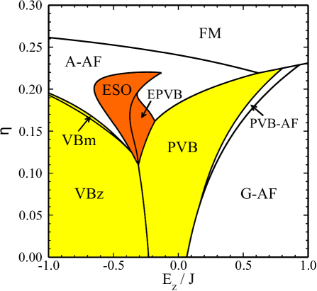
Figure 10: (Color online) The phase diagram of the cluster MF Hamiltonian (58) of the $d^{9}$ spin-orbital model for a bilayer, with independent spin (65), orbital (66) and spin-orbital (66) MFs. VB phases (mainly PVB and VB$z$) with spin disorder are stable in the light shaded (yellow) area, and phases with spin-orbital entanglement are indicated by dark grey (orange) shading. This figure is reproduced from [36].

When the spin-orbital MF (66) is not factorized but calculated self-consistently, one finds the phase diagram of figure 10. Here two $G$-AF phases for $E_{z}>0$ with occupied $x$ orbitals, $A$-AF with accompanied $C$-AO order and FM are familiar from the simplest on-site MF approach, and appear also in the 3D KK model [70]. The part of the diagram for $\eta<0.2$ and $E_{z}/J<0.5$ is dominated by two new phases compared with a one-site MF approach (shown in [36]): VB$z$ phase with $z$ orbitals occupied stable for negative $E_{z}$, and plaquette VB (PVB) phase in a range of $E_{z}\simeq 0$, both with vanishing magnetization. For small $E_{z}/J<0.25$ one finds that quantum fluctuations included within the present approach select the former spin-disordered VB$z$ phase. The latter PVB phase has singlets formed on the bonds either along the $a$ or $b$ direction of the cluster, depending on the cube. This phase breaks the $a\leftrightarrow b$ symmetry locally but the global symmetry is preserved thanks to the $\pi/2$ rotation of neighbouring clusters mentioned above. The orbitals take shape of cigars pointing in the direction of the singlets.

The most important result presented in figure 10 are the regions of stability of three new entangled phases: ESO, EPVB and PVB-AF, obtained only when the spin-orbital order parameter $u^{\gamma}_{i}$ (66) is not factorized into the spin and orbital part. ESO stands for entangled spin-orbital phase and is characterized by relatively high values of spin-orbital order parameters, especially for high values of $\eta$ when other order parameters are close to zero. This phase contains singlets along the bonds parallel to the $c$ axis, its magnetization vanishes and orbital configuration is nonuniform. EPVB stands for entangled PVB phase and resembles it, but has in addition a finite spin-orbital field, and weak global AF order. Finally, a different type of phase with spin-orbital entanglement is the PVB-AF phase connecting PVB and $G$-AF in a smooth way, stable only if $\eta$ is large enough.

Note that with the exception of this last phase, the other two entangled phases arise near the quantum critical point (QCP) which is found at $\eta=0$ in the MF approach and moves to a finite value of $\eta\simeq 0.12$ when quantum fluctuations on singlet bonds are explicitly included. Therefore, the phase diagram of figure 10 implies that singlet formation suppresses frustration caused by Hund’s exchange coupling and moves the region of the most frustrated interactions to finite $\eta$. This shows once again that the simple single-site MF approach is insufficient to describe faithfully the phase diagram of the present spin-orbital model (55). We suggest that similar entangled phases are expected in the 3D model which should be investigated within the cluster MF approach in the near future.

5.2 Spin-orbital resonating valence-bond liquid

In this section we consider another example of spin-orbital entangled states which are found in the $d^{1}$ model on the frustrated triangular lattice [37, 38], as realized in the (111) planes of NaTiO₂. In the limit of large intraorbital Coulomb interaction $U$ intersite charge excitations are again transformed away and one finds the following effective Hamiltonian [37],

$${\cal H}=J\left\{(1-\alpha)\;{\cal H}_{s}+\sqrt{(1-\alpha)\alpha}\;{\cal H}_{m}+\alpha\;{\cal H}_{d}\right\}\,,$$ (68)

where $J$ is the exchange energy for $S=\frac{1}{2}$ spins and three $t_{2g}$ orbital flavours active on a bond in different processes. Here the interaction may arise either from superexchange via oxygen orbitals due to transitions via the effective hopping $t$ that follows from the $d-p$ hybridization, or via direct (kinetic) exchange between $t_{2g}$ orbitals with flavour $\gamma$ active on a bond along the direction $\gamma$ in a triangular lattice via the hopping $t^{\prime}$. The parameter $\alpha$ interpolates between the superexchange ($\alpha=0$) and direct exchange ($\alpha=1$) limit. It is the first parameter of the present model (68) and is given by the ratio of these two hopping elements:

$$\alpha=\frac{t^{\prime 2}}{t^{2}+t^{\prime 2}}.$$ (69)

The superexchange involves two $t_{2g}$ orbital flavors (8) different from $\gamma$ on each bond that are not active in direct exchange. Consequently, the superexchange is more quantum, similar to the superexchange in titanates or vanadates, while the direct exchange is more classical in the orbital channel, bearing some similarity to the superexchange for $e_{g}$ orbitals analysed above in the bilayer KK model. The second parameter of the spin-orbital model (68) is Hund’s exchange $\eta$ (16), as in the KK model. More details on the model and its derivation can be found in [37].

In the subsequent sections we focus first on the frustrated interactions in the $d^{1}$ model (13) at $\eta=0$ limit, and we give here its explicit form in this case:

$${\cal H}_{0}\!\! = \!\!J\sum_{\langle ij\rangle\parallel\gamma}\Big{\{}(1-\alpha)\left[2\left(\vec{S}_{i}\cdot\vec{S}_{j}+\frac{1}{4}\right)\right.$$ (70)

$$\!\!\left.\times\left[\left(\vec{T}_{i}\cdot\vec{T}_{j}\right)^{(\gamma)}+\frac{1}{4}n_{i}^{(\gamma)}n_{j}^{(\gamma)}\right]\!+\frac{1}{2}(n_{i\gamma}+n_{j\gamma})-1\right]$$

$$+ \!\!\alpha\left[\left(\vec{S}_{i}\!\cdot\!\vec{S}_{j}-\frac{1}{4}\right)n_{i\gamma}n_{j\gamma}-\frac{1}{4}\Big{(}n_{i\gamma}n_{j}^{(\gamma)}+n_{i}^{(\gamma)}n_{j\gamma}\Big{)}\right]$$

$$- \!\!\frac{1}{4}\sqrt{\alpha(1-\alpha)}\;\Big{(}T_{i\bar{\gamma}}^{+}T_{j{\tilde{\gamma}}}^{+}+T_{i{\tilde{\gamma}}}^{-}T_{j\bar{\gamma}}^{-}+T_{i{\tilde{\gamma}}}^{+}T_{j\bar{\gamma}}^{+}+T_{i\bar{\gamma}}^{-}T_{j{\tilde{\gamma}}}^{-}\Big{)}\Big{\}}.$$

The summations include the bonds $\langle ij\rangle\parallel\gamma$ of a triangular lattice, with $\gamma=a,b,c$ labeling three directions. This case is rather special as the multiplet structure collapses to a single excitation with energy $U$ (spin singlet and triplet excitations are then degenerate), and the Hamiltonian simplifies. The operators $n_{i\gamma}$ are electron number operators for the orbital flavour $\gamma$ at site $i$, and $n_{i}^{(\gamma)}$ is the density in the remaining two orbitals, which is related to $n_{i\gamma}$ by the local constraint,

$$n_{i\gamma}+n_{i}^{(\gamma)}=1.$$ (71)

The scalar products of the orbital operators in (70),

$$\left(\vec{T}_{i}\cdot\vec{T}_{j}\right)^{(\gamma)}\! \equiv \frac{1}{2}\Big{(}T_{i\gamma}^{+}T_{j\gamma}^{-}+T_{i\gamma}^{-}T_{j\gamma}^{+}\Big{)}+T_{i\gamma}^{z}T_{j\gamma}^{z}\,,$$ (72)

involve two active orbital flavours on superexchange bonds. For a bond along the axis $\gamma$ orbital operators at site $i$ are defined by the electron creation $\{a_{i}^{\dagger},b_{i}^{\dagger},c_{i}^{\dagger}\}$ and annihilation $\{a_{i},b_{i},c_{i}\}$ operators for electrons with a given flavour. For instance, for the bonds along the $a$ or $b$ axis they are:

$$T_{ia}^{+}\! = \!b_{i}^{\dagger}c_{i}\,,\hskip 56.9055ptT_{ib}^{+}=c_{i}^{\dagger}a_{i}\,,$$ (73)

$$T_{ia}^{-}\! = \!c_{i}^{\dagger}b_{i}\,,\hskip 56.9055ptT_{ib}^{-}=a_{i}^{\dagger}c_{i}\,,$$ (74)

$$T_{ia}^{z}\! = \!\frac{1}{2}(n_{ib}-n_{ic})\,,\hskip 14.22636ptT_{ib}^{z}=\frac{1}{2}(n_{ic}-n_{ia})\,.$$ (75)

The labels $\bar{\gamma}\neq\tilde{\gamma}$ in the quantum fluctuating part $\propto\sqrt{\alpha(1-\alpha)}$ refer to the two orbital operators on each bond along the direction $\gamma$ involved in the fluctuating operators defined in (73). Orbital fluctuations are the only processes contributing to the mixed exchange terms in this limit ($\eta=0$).

A remarkable feature of the Hamiltonian in the limit of $\eta=0$ (70) is the lack of higher symmetry in any of the points when $\alpha$ is varied. Even at $\alpha=0.5$, where all electron transitions have the same amplitude, no higher symmetry occurs as the superexchange ($\alpha=0$) and direct exchange ($\alpha=1$) result from quite distinct processes and involve different subsets of orbital flavours which cannot be transformed one into the other. The only analytical solution was found in the $\alpha=1$ case, where at $\eta=0$ the extremely degenerate GS is a liquid of hard-core dimers [102]. This degeneracy is removed at finite $\eta>0$, and a VB crystal with a large unit cell of 20 sites is formed.

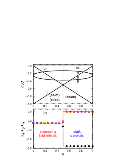
Figure 11: (Color online) Evolution of the properties of a single bond $\gamma\equiv c$ for the spin-orbital model (70) on a triangular lattice as a function of $\alpha$ at $\eta=0$: (a) energy spectrum $E_{n}$ (solid lines) with degeneracies given by numbers; (b) spin $S_{ij}$ (19) (filled circles), orbital $T_{ij}$ (20) (empty circles), and spin–orbital $C_{ij}$ (21) ($\times$) correlations. The transition between the two distinct regimes occurs by a level crossing at $\alpha=0.5$. For $\alpha<0.5$, the two types of dimer wave function [(ss/ot) and (os/st)] are degenerate ($d=6$) for resonating orbital configurations $\{ab\}$, while at $\alpha>0.5$, the nondegenerate spin singlet is supported by $c$ orbitals occupied at both sites [(ss/cc)]. This figure is reproduced from [37].

To understand a subtle interplay between the quantum superexchange at $\eta=0$ and more classical direct exchange in the limit of $\eta=1$ we consider first a single bond oriented along the $c$ axis. In the superexchange limit the active orbitals are $a$ and $b$, while only $c$ orbitals contribute to the direct exchange (70). A single bond gives the GS energy $E_{0}=-J$, both in the superexchange ($\alpha=0$) and in the direct exchange ($\alpha=1$) limit, see figure 11(a). These two limits differ in a fundamental way — the GS at $\alpha=0$ has degeneracy $d=6$ due to two complementary triply degenerate wave functions, with spin singlet and orbital triplet (ss/ot), and spin triplet accompanied by orbital singlet (st/os), while in the opposite $\alpha=1$ case limit spin singlet is accompanied by frozen FO order of active $c$ orbital (ss/cc). Energy increase when the $\alpha=0.5$ point is approached from either side indicates increasing frustration.

The different character of wave functions prevents any energy gain that might result from orbital fluctuations in the mixed exchange term, and the GS energy $E_{0}$ increases linearly toward $E_{0}=-\frac{1}{2}J$ when the point $\alpha=0.5$ is approached from either side. At this point the interactions are maximally frustrated, degeneracy is $d=7$, and a QPT between the two described GSs takes place. Also the remaining part of the spectrum (excited states) is symmetric with respect to the $\alpha=0.5$ point. Altogether, the evolution of the spectrum with $\alpha$ demonstrates not only that superexchange and direct exchange are physically distinct, excluding each other and unable to contribute at the same time, but also that the two wave functions optimal in either limit are extremely robust.

The above interpretation is consistent with the spin, orbital, and composite spin-orbital correlation functions for the considered bond, defined in equations (19)-(21). In the entire regime of $0\leq\alpha<0.5$, averaging over two degenerate (ss/ot) and (st/os) wave functions leads to equal spin and orbital correlation functions $S_{ij}=T_{ij}=-\frac{1}{4}$, see figure 11(b). As a singlet for one quantity is matched by a triplet for the other one, the two sectors are strongly correlated, and one also finds $C_{ij}=-\frac{1}{4}$. Although individual quantum states may be written here as products of the respective spin and orbital states, this result suggests that strong spin-orbital entanglement in expected in the GS of a larger system. It may be shown that entanglement arises there mathematically because the GS is a resonating superposition of a number of configurations [38] which do not couple here with one another and form degenerate states for a single bond. Note that the obtained value, $C_{ij}=-\frac{1}{4}$, is the same as in the SU(4) model, see section 3.2, and reflects maximal possible entanglement.

By contrast, for $\alpha>0.5$ the above degenerate states favoured by superexchange become excited states, and the spin-singlet GS ($S_{ij}=-\frac{3}{4}$) is the lowest, see figure 11(b). The orbital configuration is characterized here by a rigid order of $c$ orbitals, $\langle n_{ic}n_{jc}\rangle=1$, which quenches all orbital fluctuations. Thus the spin and orbital parts are trivially decoupled, giving $C_{ij}=0$. Finally, at the transition point $\alpha=0.5$ one finds degeneracy $d=7$ and averaging over all degenerate states yields $S_{ij}=-0.321$, $T_{ij}=-0.214$, and somewhat reduced composite function $C_{ij}\simeq-0.23$, as one of the degenerate states gives here $C_{ij}=0$. Summarizing, the regime of entangled spin-orbital states $\alpha<0.5$ is complemented by a factorized (disentangled) (ss/cc) wave function.

Below we analyse how the above two distinct regimes of the $d^{1}$ model are modified in case of large number of neighbours and frustration in the triangular lattice. We consider two clusters with PBC: a hexagonal cluster of $N=7$ sites (N7), and a rhombic cluster of $N=9$ sites (N9). Unfortunately, the cluster with even $N=12$ number of sites is too large and would require very extensive calculations, but the presented clusters are sufficient to demonstrate essential differences between the nature of interactions in both limits. Due to the PBC all sites and bonds are equivalent, so bond correlations are all the same and independent of the bond direction $\gamma$. Each $t_{2g}$ orbital is occupied on average by 1/3 electron, but similar to a single bond the GSs are manifestly different in the limits of $\alpha=0$ and $\alpha=1$, see the insets in figure 12(b).

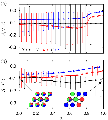
Figure 12: Bond correlations for clusters with PBC at $\eta=0$ — spin ${\cal S}$ (19), orbital ${\cal T}$ (20), and spin-orbital ${\cal C}$ (21): (a) hexagonal cluster of $N=7$ sites, and (b) rhombic cluster of $N=9$ sites. Vertical lines indicate the exactly determined range of possible values of each quantity at a given $\alpha$ that follows from the GS degeneracy. The insets in (b) indicate typical orbital patterns in the superexchange ($\alpha=0$) and direct exchange ($\alpha=1$) limit for the rhombic N9 cluster; a more symmetric hexagonal cluster N7 is obtained by removing top-right and bottom-left sites. These data were presented in [38].

In case of N7 cluster all three directions are equivalent and the spin correlations are AF and constant, $S_{ij}\simeq-0.11$ independently of $\alpha$. Note that this value can be deduced as follows: In the low-spin phase one has ${\cal S}_{t}=\frac{1}{2}$ total spin, and one can determine the intersite spin correlations using the following identity [38]:

$$\vec{\cal S}^{2}=7\vec{S}_{i}^{2}+42\langle\vec{S}_{i}\cdot\vec{S}_{j}\rangle\,.$$ (76)

Due to PBC every pair of sites stands for a nearest neighbour bond and this implies the above relation. The value $\langle\vec{S}_{i}\cdot\vec{S}_{j}\rangle=-3/28=-0.107$ obtained from it reflects AF spin correlations but is much reduced from the classical limit of $-0.25$ found in the Néel state on a square lattice, in agreement with high frustration of the triangular lattice. Note that the present situation is radically different from the 1D SU(4) model, where frustration is absent but spin correlations are reduced by their coupling to the orbital correlations. In the N9 cluster spin correlations are in a similar range but vary somewhat with $\alpha$ as the cluster shape breaks the symmetry between bonds in three nonequivalent directions $\{a,b,c\}$. These correlations are weaker (${\cal S}\simeq-0.090$) at $\alpha=0$ than in the N7 cluster and become more pronounced (${\cal S}\simeq-0.144$) when $\alpha\simeq 0.6$, while orbital fluctuations gradually weaken to ${\cal C}\simeq-0.050$ at $\alpha=1$.

In both clusters orbital correlations are negative, ${\cal T}<0$, and the Goodenough-Kanamori rule stating that these correlations should be complementary to spin ones is violated. The orbital correlations weaken in both clusters when $\alpha$ increases towards $\alpha=1$ and the superexchange interactions are less important, particularly in the N9 cluster. Joint spin-orbital correlations are also similar in both clusters (e.g. ${\cal C}\simeq-0.070$ at $\alpha=0$) and $|{\cal C}|$ gradually decreases when spin and orbitals disentangle approaching $\alpha=1$.

An important question is whether spin order and excitations could be described by an effective spin model derived from the spin-orbital model (13). Below we show that this is not the case in the $d^{1}$ model on the triangular lattice. MF procedure used frequently leads here to [38]:

$${\cal H}_{\rm MF} = \sum_{\langle ij\rangle\parallel\gamma}\left\{\left\langle{\hat{\cal J}}_{ij}^{(\gamma)}\right\rangle{\vec{S}}_{i}\cdot{\vec{S}}_{j}-\left\langle{\hat{\cal J}}_{ij}^{(\gamma)}\right\rangle\left\langle{\vec{S}}_{i}\cdot{\vec{S}}_{j}\right\rangle\right\}$$ (77)

$$+ \sum_{\langle ij\rangle\parallel\gamma}\left\{{\hat{\cal J}}_{ij}^{(\gamma)}\left\langle{\vec{S}}_{i}\cdot{\vec{S}}_{j}\right\rangle+{\hat{\cal K}}_{ij}^{(\gamma)}\right\}\,.$$

In this way spin and orbital degrees of freedom are disentangled and the model reduces to a superposition of the spin model with self-consistently determined orbital correlations, and the orbital model, with self-consistently derived spin correlations, similar to the decoupling of spin and orbital degrees of freedom introduced for the 1D spin-orbital chain in section 4.3. Following the spin model, one obtains the MF spin interactions for N7 and N9 clusters by averaging the orbital operator ${\hat{\cal J}}_{ij}^{(\gamma)}$ (its explicit form is given in [38]) over the MF GS $|\Phi_{0}\rangle$ (14). Note that the orbital fluctuations in the term $\propto\sqrt{\alpha(1-\alpha)}$ in (70) contribute here as well as they couple different components of $|\Phi_{0}\rangle$. In contrast, the exact exchange constant $J_{\rm exact}$ (30) is found when the exact GS $|\Phi\rangle$ obtained after Lanczos diagonalization is used for a given cluster.

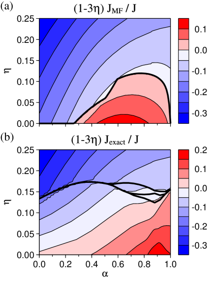
Figure 13: (Color online) Contour plots of the effective exchange constant $J_{\rm MF}$ as obtained for the hexagonal cluster of $N=7$ sites with PBC: (a) within the MF calculation which includes orbital fluctuations (14), and (b) using the exact GS found in exact diagonalization (30). In case (a) the transition from low-spin to high-spin phase occurs when the exchange constant $J_{\rm MF}$ changes sign and becomes negative. Thick lines in (b) indicate the phase boundaries between phases with increasing intermediate total spin value ${\cal S}_{t}=3/2$, 5/2 between ${\cal S}_{t}=1/2$ and 7/2 for increasing $\eta$. This figure is reproduced from [38].

In figure 13 we compare the phase diagrams obtained from the above MF procedure and from Lanczos diagonalization for the N7 cluster. Consider first a QPT from the low-spin (${\cal S}_{t}=1/2$) disordered phase to the high-spin (${\cal S}_{t}=7/2$) FM phase which occurs for sufficiently large $\eta$. When spin and orbital operators are disentangled (77), see figure 13(a), and ${\cal C}\equiv 0$, it coincides with the sign change of the MF exchange constant $J_{\rm MF}$ (14) and no intermediate phase (with $1/2<{\cal S}_{t}<7/2$) is found, as in a spin system.

Comparing the values of $J_{\rm MF}$ (14) and $J_{\rm exact}$ (30) found from the MF and from exact diagonalization of the N7 cluster, see figure 13, one finds that $J_{\rm exact}\geq J_{\rm MF}$ in a broad range of $\alpha$. Therefore, the MF approximation turns out to be rather unrealistic and overestimates (underestimates) the stability of states with FM (AF) spin correlations. The value of $J_{\rm MF}$ decreases with increasing $\eta$, but positive values $J_{\rm MF}>0$ are found at $\eta=0$ only if $0.27<\alpha<1$. This demonstrates that FM states: ($i$) are favoured when joint spin-orbital fluctuations are suppressed, and ($ii$) are stabilized by orbital fluctuations close to $\alpha=0$ even in absence of Hund’s exchange. The transition from the low-spin (${\cal S}_{t}=1/2$) to the high-spin (${\cal S}_{t}=7/2$) state occurs in Lanczos diagonalization at a much higher finite value of $\eta\approx 0.14$, with only weak dependence on $\alpha$, see figure 13(b). In addition, one finds two phases with intermediate spin values ${\cal S}_{t}=3/2,5/2$ in a range of $\eta$ values near $\alpha=0.8$. Note that the exchange constant $J_{\rm exact}$ changes discontinuously at the onset of the FM phase.

We have found that the qualitative trends presented here for the N7 cluster are similar to those observed for the N7 cluster [103] and thus they may be considered generic for the present $d^{1}$ model on the triangular lattice. In both cases one finds that: ($i$) the FM phase is stable in the MF approximation close to $\alpha=0$ and becomes degenerate with the low-spin phase at $\alpha=1$, ($ii$) the MF procedure is exact in the regime of FM phase, and ($iii$) the transition to the FM phase occurs gradually through intermediate values of total spin ${\cal S}_{t}$ (except at $\alpha=1$). This suggests that partially polarized FM phase should occur in the thermodynamic limit. It arises due to spin-orbital entanglement which is gradually suppressed when $\eta$ increases.

We argue that the results presented in [38] and [103] provide evidence that the present $d^{1}$ spin-orbital model realizes a paradigm of a spin-orbital liquid phase in the superexchange regime, and the order-out-of-disorder mechanism does not occur when the Hilbert space contains coupled spin and orbital sectors. Previous search for this quantum state of matter in other systems, particularly in LiNiO₂ where $e_{g}$ orbitals are active on the $d^{7}$ configurations of Ni³⁺ ions on the triangular lattice [104], were unsuccessful [105, 106]. After considering the present model in more detail we suggest that the triple degeneracy of $t_{2g}$ orbitals plays a crucial role in the onset of a spin-orbital liquid, as the number of orbital flavours fits to the geometry of the triangular lattice. In contrast, the direct exchange regime is dominated by VB states with spin singlets accompanied by static configurations of directional orbitals providing the energy gain for the direct exchange. Note that the frustrated triangular lattice plays here an important role and removes any kind of orbital order in the entire range of $\alpha$.

6 Hole propagation in a Mott insulator with coupled spin-orbital order

Finally, we give an example of a single hole doped into the half-filled Mott insulator with a pseudo-entangled AF/AO order [34]. This type of order is realized in the $ab$ planes of LaVO₃ with $S=1$ spins [21] and in Sr₂VO₄ with $S=\frac{1}{2}$ spins [107]. It might appear as entangled as it contradicts the Goodenough-Kanamori rules and has certain similarity to the entangled spin-orbital states in a 1D chain, see section 3.3. It is well known that a hole doped into a quantum antiferromagnet couples to the collective (delocalized) spin excitations (magnons), and propagates through the lattice surrounded by a ”cloud” of magnons which is the essence of a QP behaviour [108]. Thereby the energy scale of the ”coherent” hole propagation is strongly renormalized from the hopping $t$ and is given by the AF superexchange constant $J$. This QP is frequently called a spin polaron [28] and was observed in the photoemission spectra of the parent compounds of high-$T_{c}$ cuprates, as e.g. in Sr₂CuO₂Cl₂ [109].

A hole doped in a Mott insulator with orbital order could behave in a similar way when orbital fluctuations or interorbital hopping [30] would also repair the defects created by a hole. Orbital excitations are decoupled from spin ones in disentangled states, such as FM spin and AO order in the $ab$ planes of LaMnO₃ [12]. It has been shown [30] that a hole introduced into such a state indeed does not disturb the FM spin order and couples to the collective excitations of the AO state (orbitons). Here again a QP is formed which is called this time an orbital polaron [110]. Usually, however, the bandwidth of an orbital polaron is much smaller than that of the spin one. In fact, the orbitons are in general considerably less mobile than the magnons (or even immobile) due to almost directional Ising-like superexchange [12, 43]. Actually, one can understand the hole motion in this case in terms of the string picture [112, 111].

The orbital order created by $t_{2g}$ orbitals in a 2D square lattice is more robust than that of $e_{g}$ ones while only 1D hopping for each orbital flavour is allowed in the former case [31]. The case of a hole doped into the plane with FM spin order accompanied by the $t_{2g}$ AO order, which could correspond not only to the hole introduced into the ordered ground state of Sr₂VO₄ with $t_{2g}$ orbitals but also, surprisingly, to K₂CuF₄ or Cs₂AgO₄ with active $e_{g}$ orbitals. As the GS has AO order, also here a QP might formed due to the dressing of a hole by the collective orbital excitations. However, due to the specific $t_{2g}$ orbital symmetries the orbitons are not mobile at all, and the QP acquires a finite bandwidth only due to the frequently neglected three-site terms [31]. Thus, the string picture determines the nature of the $t_{2g}$ orbital polarons even more than in systems with $e_{g}$ orbital degrees of freedom.

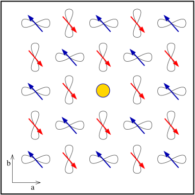
Figure 14: Artist’s view of a single hole introduced into the spin and orbitally ordered $ab$ plane of LaVO₃ with coexisting AF/AO order. One electron at each V³⁺ ion occupies the $xy$ orbital (not shown) and the other one either $yz$ or $zx$ degenerate orbital, forming the classical AO state (the projections of these orbitals onto the $ab$ plane are shown) whereas their spins $S=\frac{1}{2}$ alternate on two sublattices, forming the AF Néel state. This figure is reproduced from [34].

A more complex situation arises, however, when a doped hole may couple in a $t_{2g}$ system both to magnon and to orbiton excitations [66]. This situation is found in the $ab$ plane of LaVO₃, shown schematically in figure 14 and studied in [34]. The coexisting AF/AO order consists of the AF order induced by the superexchange interactions between the occupied $c$ orbitals, and the AO order of active $\{a,b\}$ orbitals. The GS in an undoped system is therefore a perfect two-sublattice order, with quantum fluctuations in the spin channel but a classical AO order in the orbital channel as the superexchange interations in this part are Ising-like. The coexistence of the AO and AF order is extremely rare as it formally violates [1] the Goodenough-Kanamori rules predicting complementary spin and orbital order in the GS. This GS has long-range order, with an up (down) spin component accompanied by a $zx$ ($yz$) orbital, but this composite nature of the GS has no dramatic consequences as long as the system is undoped.

The problem of a single hole doped into the $ab$ plane of LaVO₃, see figure 14, is challenging as the hole doping occurs in the orbital $\{a,b\}$ doublet and disturbs locally both AF and AO order [113]. Unlike in the FM/AO case [32], for the present coexisting AF/AO order neither the spin nor the orbital background is transparent for a propagating hole, and the hole has to couple simultaneously to both magnons and orbitons when it moves by one lattice spacing. It is then unclear whether a QP may form and which role is played individually by spins and orbitals in possible formation of a spin-orbital polaron.

The 2D spin-orbital $t$-$J$ model may be seen as a generalization of the spin $t$-$J$ model [64] and the orbital $t_{2g}$ $t$-$J$ model [31] to the spin-orbital superexchange — it consists of three terms [34],

$$H=H_{t}+H_{J}+H_{3s},$$ (78)

where the last one, $H_{3s}$, stands for the three-site effective hopping. The second term $H_{J}$ is the spin-orbital superexchange model for the $R$VO₃ perovskites (13) introduced above in section 4.1. The first term in (78) describes the hopping of $\{a,b\}$ electrons in the constrained Hilbert space, i.e., in the space with singly occupied (at hole position) or doubly occupied sites. This means that electrons in the $ab$ plane, which is under consideration here, can hop only along the $b$ ($a$) direction when they carry $a$ ($b$) orbital flavour. The $c$ orbitals do not participate in hopping processes as they are always occupied by one electron (29), see [80, 114]. Hence, we arrive at the kinetic $\propto t$ part of Hamiltonian (78),

$$H_{t}=-t\sum_{{\bf i},\sigma}{\cal P}\left(\tilde{b}^{\dagger}_{{\bf i}\sigma}\tilde{b}_{{\bf i}+\hat{\bf a}\sigma}+\tilde{a}^{\dagger}_{{\bf i}\sigma}\tilde{a}_{{\bf i}+\hat{\bf b}\sigma}+{\rm H.c.}\right){\cal P}.$$ (79)

Here the constrained operators $\tilde{a}^{\dagger}_{{\bf i}\sigma},\{\tilde{b}^{\dagger}_{{\bf i}\sigma}\}$ mean that the hopping is allowed only in the restricted Hilbert space with not more than one $\{a,b\}$ electron at each site ${\bf i}$ ($\bar{\sigma}$ stands for the spin component opposite to $\sigma$). Besides, since Hund’s exchange coupling is large ($J_{H}\gg t$) [115], we project the final states resulting from the electron hopping onto the high-spin states, which occurs due to the ${\cal P}$ operators in (79). More details can be found in [34].

Low energy excitations are magnons and orbitons, with their energies determined by the respective exchange constants derived from the spin-orbital superexchange [34],

$$J_{S} = \frac{1-3\eta-5\eta^{2}}{4(1-3\eta)(1+2\eta)}\,J\,,$$ (80)

$$J_{O} = \frac{\eta(2-\eta)}{(1-3\eta)(1+2\eta)}\,J\,.$$ (81)

One finds that $J_{O}>0$ and $J_{S}>0$ in the expected range of $\eta<0.2$, which means that the classical GS has indeed coexisting AF and AO order. By rotating first spins and orbitals at sublattice $A$ to the FM/FO order and introducing Schwinger bosons $f^{\dagger}_{{\bf i}\sigma}$ for spin and $t^{\dagger}_{{\bf i}\alpha}$ for orbital excitations, one finds the energies of magnons and orbitons using the LSW theory. As usually in a quantum antiferromagnet, magnons are dispersive and have a Goldstone mode,

$$\omega_{\bf k}=J_{S}zS\sqrt{1-\gamma^{2}_{\bf k}}\,,$$ (82)

where $\gamma_{\bf k}$ is given by (53), $S=1$ and $z=4$ is the coordination number. In contrast, the orbital excitations at energy $J_{O}$ are local and have no dispersion as the orbital interactions are Ising-like.

A crucial step in deriving the hole spectral function $A({\bf k},\omega)$ is the following representation of the electron operators in terms of the $\{f^{\dagger}_{{\bf i}\sigma},t^{\dagger}_{{\bf i}\alpha}\}$ ($\alpha=a,b$) Schwinger bosons:

$$\tilde{a}^{\dagger}_{{\bf i}\sigma} = \frac{1}{\sqrt{2}}f^{\dagger}_{{\bf i}\sigma}t^{\dagger}_{{\bf i}a}h_{\bf i}\,,$$ (83)

$$\tilde{b}^{\dagger}_{{\bf i}\sigma} = \frac{1}{\sqrt{2}}f^{\dagger}_{{\bf i}\sigma}t^{\dagger}_{{\bf i}b}h_{\bf i}\,.$$ (84)

The above equations demonstrate that a spin excitation is always generated together with an orbital excitation, which implies that the diagrams contributing to the self-energy contain only vertices with two outgoing or incoming excitation lines. The factor $\frac{1}{\sqrt{2}}$ follows from spin algebra for spins $S=1$ in the spin-orbital model [34]. Here the projection onto the high-spin states has already been done, so the projection operators ${\cal P}$ in $H_{t}$ are no longer needed.

The spectral function can be obtained from the Green’s functions which are defined separately for ${\cal A}$ and ${\cal B}$ sublattice and depend on the corresponding self-energy $\Sigma_{\alpha}({\bf k},\omega)$ ($\alpha=a,b$):

$$G_{\alpha}({\bf k},\omega)=\frac{1}{\omega+\varepsilon_{\alpha}({\bf k})-\Sigma_{\alpha}({\bf k},\omega)}\,.$$ (85)

Here $\varepsilon_{a}({\bf k})=2\tau\cos(2k_{y})$ and $\varepsilon_{b}({\bf k})=2\tau\cos(2k_{x})$, and $\tau=\frac{1}{4}J$ describes the three-site hopping responsible for the 1D dispersion within each sublattice. In what follows we show only the result for $\tau=0$ for more clarity. Green’s functions are solved self-consistently together with the self-energies derived in the self-consistent Born approximation (SCBA). After solving the Green’s functions, the spectral functions for a hole created in $\alpha=\{a,b\}$ orbital are:

$$A_{\alpha}({\bf k},\omega)=-\frac{1}{\pi}\lim_{\delta\to 0}\,\mbox{Im}\,G_{\alpha}({\bf k},\omega+i\delta)\,.$$ (86)

At $\tau=0$ the spectral function does not depend on the orbital flavour, and we define $A({\bf k},\omega)\equiv A_{\gamma}({\bf k},\omega)$.

The spectral functions $A({\bf k},\omega)$ (86) shown in figure 15 are representative for the situation in the strongly correlated transition metal oxides. They are obtained by solving the SCBA equations for $J=0.4t$ on a mesh of $16\times 16$ ${\bf k}$-points. Similar data for other values of $J=0.2t$ and $0.6t$ are presented in [34]. A realistic value of Hund’s exchange in LaVO₃ is $\eta=0.15$ [71]. The peak in the low-energy part of the spectrum, see figure 15(c), has no dispersion which indicates hole confinement (a rather weak 1D dispersion along the $k_{x}$ ($k_{y}$) direction for holes doped into the $b$ ($a$) orbitals is obtained at finite $\tau=\frac{1}{4}J$). The spin-orbital spectral functions form ladder-like spectra and have many similarities with the spectra obtained for the $t_{2g}$ orbital $t$-$J$ model [31]. However, there are few subtle differences with the orbital model which demonstrate that the spin-orbital case is more complex and the spin part also contributes.

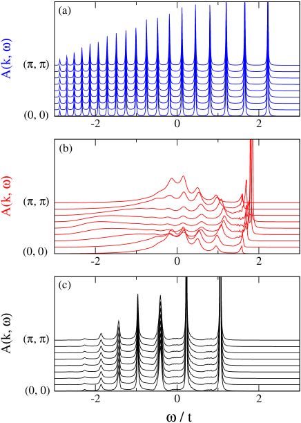
Figure 15: Spectral functions for a single hole in the AF/AO phase along the $\Gamma-M$ direction of the Brillouin zone for: (a) toy orbital model (88) (top); (b) toy spin model (87) (middle); (c) the full spin-orbital model (13) (bottom). Parameters: $J=0.4t$ and $\eta=0.15$ (i.e., $J_{S}=0.06t$ and $J_{O}=0.16t$). Broadening $\delta=0.01t$ in the definition (86) of the spectral function is assumed. Image courtesy of Krzysztof Wohlfeld.

To understand better the nature of the obtained spectra we present also the spectral functions obtained for the related spin and orbital problem in figure 15(a-b). These two models read as follows [34]:

$$H_{S} = -t\sum_{\langle{\bf i}{\bf j}\rangle,\sigma}{\cal P}(\tilde{c}^{\dagger}_{{\bf i}\sigma}\tilde{c}_{{\bf j}\sigma}+{\rm H.c.}){\cal P}+J_{S}\sum_{\langle{\bf i}{\bf j}\rangle}{\bf S}_{\bf i}\cdot{\bf S}_{\bf j}\,,$$ (87)

$$H_{O} = -t\sum_{\bf i}\left(\tilde{b}^{\dagger}_{\bf i}\tilde{b}_{{\bf i}+\hat{\bf a}}+\tilde{a}^{\dagger}_{{\bf i}}\tilde{a}_{{\bf i}+\hat{\bf b}}+{\rm H.c.}\right)+J_{O}\sum_{\langle{\bf i}{\bf j}\rangle}T^{z}_{\bf i}T^{z}_{\bf j}.$$ (88)

Here spin operators $\{{\bf S}_{\bf i}\}$ stand for $S=1$ spins, $T^{z}_{i}$ are $z$th components of pseudospin $T=1/2$, and the operators ${\cal P}$ project onto the high-spin states. The constrained electron operators, $\tilde{c}^{\dagger}_{{\bf i}\sigma}=c^{\dagger}_{{\bf i}\sigma}(1-n_{{\bf i}\bar{\sigma}})$ in (87) and $\tilde{b}^{\dagger}_{\bf i}=b^{\dagger}_{\bf i}(1-n_{{\bf i}a})$ and $\tilde{a}^{\dagger}_{\bf i}=a^{\dagger}_{\bf i}(1-n_{{\bf i}b})$ in (88) exclude double occupancies from the Hilbert space in each case, similar to (79). The superexchange energy scale is $J_{S}$ (80) for the spin model (87) and $J_{O}$ (81) for the orbital one (88), which mimics the influence of the orbital part on the spins and of the spin part (with the AF order) on the orbitals. With the present parameters one finds the spin-only exchange constant $J_{S}=0.06t$ (somewhat higher than that deduced from the observed value of the Néel temperature $T_{N}\simeq 143$ K in LaVO₃ [21]), and $J_{O}=0.16t$.

The spectral functions for the above models were obtained using the SCBA on a mesh of $16\times 16$ ${\bf k}$-points, following the derivations presented in [28] and [32] in the case of the spin and orbital model. One only has to make the following substitutions in the respective SCBA equations: $J\rightarrow-J_{S}$, $S\rightarrow 1$ and (due to the quantum double exchange factor) also $t\rightarrow t/\sqrt{2}$ in the spin case [28], and $J\rightarrow-J_{O}$, $E_{0}\rightarrow 0$, and $\tau\rightarrow 0$ in the orbital case [32]. The spectral functions obtained for the above toy models are quite different from those obtained for the spin-orbital $t$-$J$ model. The spectral function for the spin model, see figure 15(b), consists of a QP and the incoherent part at higher energies, both having considerable ${\bf k}$-dependence. It is evident that this ${\bf k}$-dependence is removed by the orbital interactions. The orbital model at $\tau=0$ has a strictly localized spectral function with a ladder spectrum [28], see figure 15(a). The spin-orbital spectral function, see figure 15(c), resembles qualitatively the ladder spectrum found for the orbital model in figure 15(a). The momentum dependence of both the QP state and the incoherent part of the spectrum obtained for the spin model, see figure 15(b), is entirely suppressed. These results demonstrate that the quantum spin fluctuations are to a large extent quenched in the spin-orbital model by the simultaneous coupling of the hole to both spin and orbital excitations. It is remarkable that the hole still couples to the spin degrees of freedom by generating string potential due to defects created by hole motion. Thus, the string which acts on the hole moving in the plane with AF/AO order is of the composite spin-orbital character. This not only explains the peculiar correspondence between the orbital and spin-orbital model, but also shows that the spins play an active role in the lightly doped spin-orbital system.

We remark that the orbitally induced string formation considered here could be understood as a topological effect. It happens even if the orbital excitation energy is turned to zero, i.e., when the hole moves in the orbital sector incoherently. Hence, the mere presence of orbitals is sufficient to obtain the (almost) classical behaviour of a hole doped into the GS with AF/AO order. This result suggests that further investigation of the hole propagation in spin-orbital systems is a fascinating subject for future studies.

7 Discussion and summary

Spin-orbital entanglement discussed in this topical review concerns entanglement on the exchange bonds, similar to entanglement in e.g. spin singlets which build VB states [39, 40]. We have shown that this concept is important is several spin-orbital models and in general either the ground state or excited states are entangled. Two recent examples of entangled ground states were presented: the Kugel-Khomskii model on a bilayer, and the spin-orbital $d^{1}$ model on the triangular lattice, in addition to the well known 1D SU(2)$\otimes$SU(2) model. It may be expected that more spin-orbital model systems with entangled ground states will be found in the near future. Whether or not such states are indeed realized in nature depends on the coupling to the lattice. For instance, the $e_{g}$ orbital order is robust in LaMnO₃ [12] and KCuF₃ [99], and for this reason the ground states of these compounds are disentangled.

We have also demonstrated that the Goodenough-Kanamori rules are violated in the regime of weak Hund’s exchange in several situations. It is in this regime that the mean field decoupling procedure of spin and orbital operators fails and the magnetic properties can be determined only by solving the full entangled spin-orbital many-body problem. Also for weak (or vanishing) Hund’s exchange spin-orbital liquid phase is stabilized by spin-orbital entanglement in the $d^{1}$ spin-orbital model on the triangular lattice.

However, a frustrated lattice does not guarantee that a disordered spin-orbital liquid-like state arises. A good counterexample is the frustrated lattice of alkali $R$O₂ hyperoxides (with $R$=K, Rb, Cs), where the interactions induced by the lattices compete with the superexchange and stabilize the orbital order, lifting the geometric frustration of the lattice [116]. Then the spin-orbital interactions may be consideed as disentangled, and the Goodenough-Kanamori rules require certain reinterpretation. In fact, they have been generalized by including large interorbital hopping terms [116].

It has been shown that ground states which contradict the celebrated Goodenough-Kanamori rules may appear in two different situations: ($i$) either when quantum fluctuations in the spin-orbital system are strong and stabilize the entangled ground state with coexisting AF and AO order, or ($ii$) when the AF superexchange interactions follow from charge excitations in other orbitals not involved the actual orbital order, or ($iii$) when the coupling to the lattice stabilizes the AO order in the regime where the AF spin correlations are expected due to superexchange. In these latter situation the ground state is more classical and not entangled as it follows from interactions induced by the lattice and not from the spin-orbital superexchange. Also in the regime of large Hund’s exchange $J_{H}$, ground states with coexisting FM and FO order may appear [117], similar to the FM/FO states in the SU(2)$\times$SU(2) model. They contradict again the Goodenough-Kanamori rules, but are in fact disentangled — here quantum fluctuations are absent and play no role for their stability.

On the example of the $R$VO₃ perovskites we have shown that the experimental data in this unique family of correlated oxides indicate that low-energy excited states are entangled and the energies of spin and orbital excitations are similar. This happens because lattice distortions and interactions of $t_{2g}$ orbitals with Jahn-Teller modes are weak and only the electronic interactions such as superexchange decide about the system behaviour. In the $R$VO₃ systems the temperature dependence of the optical spectral weight, the phase diagram as a function of the ionic radius of $R$ ions, and the dimerized magnon excitations, are all determined by the presence of entangled states with low excitation energies.

The interplay between spin, orbital and spin-orbital excitations poses a very interesting problem for future theoretical studies as well as an experimental challenge. We also point out that in case of FO order accompanied by AF interactions, spin fluctuations couple to orbital excitations and thus they cannot be considered separately [118], in spite of formal separation of spin and orbital degrees of freedom in the ground state. Another important finding is recent observation that composite spin-orbital excitations fractionalize in the quasi-1D Mott insulator Sr₂CuO₃ [119]. The nature of spin-orbital excitations and the circumstances of their possible decay are very challenging and unresolved questions. The case considered here of a hole moving in the AF/AO order [34] seems to suggest that, at least in doped systems, spin-orbital excitations may play a very important role in transport as they may not decay and impose some topological constraints on carrier propagation.

The present topical review focused on spin-orbital entanglement on the superexchange bonds, but a different kind of entanglement arises in presence of on-site relativistic spin-orbit interaction. In this case a Kramers doublet gives the lowest energy states of a single ion and these states are next considered to derive interactions between neighbouring ions [120]. Such local on-site entangled states play an important role and decide about the magnetic properties of Sr₂IrO₄ with weak ferromagnetism and Sr₂VO₄ with hidden spin-orbital order. In a 1D superexchange model with Ising-like orbital superexchange locally entangled states introduce orbital dynamics and lead to a phase diagram with a novel phase having long-range Néel order of spin and orbital angular momenta [121]. Excitations is such models are a challenge and they are under investigation at present. If localized states with an effective angular momentum ${\vec{J}}_{i}=2{\vec{S}}_{i}-{\vec{L}}_{i}$ at site $i$ (with ${\vec{S}}$ and ${\vec{L}}$ being spin and orbital operators) are considered, one finds a gapped spectrum at finite spin-orbit coupling [122].

Finally, we would like to emphasize that a better understanding of the concept of spin-orbital entanglement is important and could help to make progress in other fields as this subject is interdisciplinary. Recently a scheme to generate spin-orbit-path hybrid Greenberg-Horne-Zeilinger entanglement [123] was proposed [124] for photons which are entangled with different degrees of freedom. In quantum chemistry entanglement is considered in chemical bonds which are classified using measures of electron correlation [125] and entanglement [126]. Spin-orbital-like entanglement is also applicable to nuclear systems, where nucleons possess as well two degrees of freedom — spin and isospin. It has been established that the entanglement length of the nucleons is significantly larger than that one expects [78]. Entanglement may also play an important role in quantum computations if the spin state used for information storage would be measured by investigating orbital qubits in entangled states [127].

References

References

- [1] Oleś A M, Horsch P, Feiner L F and Khaliullin G 2006 Phys. Rev. Lett. 96 147205
- [2] Nielsen M A and Huang I L 2000 Quantum Computation and Information (Cambridge University Press, Cambridge, England)
- [3] Bengtsson I and Życzkowski K 2006 Geometry of Quantum States — An Introduction to Quantum Entanglement (Cambridge University Press, Cambridge, England)
- [4] Horodecki R, Horodecki P, Horodecki M and Horodecki K 2009 Rev. Mod. Phys. 81 865
- [5] Amico L, Fazio R, Osterloh A and Vedral V 2008 Rev. Mod. Phys. 80 517
-
[6]
Amico L and Fazio R 2009
J. Phys. A: Math. Theor. 42 504001
Latorre J I and Riera A 2009 J. Phys. A: Math. Theor. 42 504002 - [7] Peschel I and Eisler V 2009 J. Phys. A: Math. Theor. 42 504003
- [8] Bloch I 2008 Nature 453 1016
- [9] Affleck I, Laflorencie N and Sorensen E 2009 J. Phys. A: Math. Theor. 42 504009
- [10] Kugel K I and Khomskii D I 1982 Sov. Phys. Usp. 25 231
- [11] Oleś A M 2009 Acta Phys. Polon. A 115 36
- [12] Feiner L F and Oleś A M 1999 Phys. Rev. B 59 3295
- [13] Oleś A M, Khaliullin G, Horsch P and Feiner L F 2005 Phys. Rev. B 72 214431
-
[14]
Goodenough J B 1963
Magnetism and the Chemical Bond
(Interscience, New York)
Kanamori J 1959 J. Phys. Chem. Solids 10 87 -
[15]
Dagotto E, Hotta T and Moreo A 2001
Phys. Rep. 344 1
Dagotto E 2005 New J. Phys. 7 67 - [16] Kovaleva N N, Oleś A M, Balbashov A M, Maljuk A, Argyriou D N, Khaliullin G and Keimer B 2010 Phys. Rev. B 81 235130
- [17] Weiße A and Fehske H 2004 New J. Phys. 6 158
-
[18]
Daghofer M, Oleś A M, Neuber D M and von der Linden W 2006
Phys. Rev. B 73 104451
Daghofer M and Oleś A M 2007 Acta Phys. Polon. A 111 497 -
[19]
Rościszewski K and Oleś A M 2007
J. Phys.: Condensed Matter 19 186223
Rościszewski K and Oleś A M 2008 J. Phys.: Condensed Matter 20 365212
Rościszewski K and Oleś A M 2010 J. Phys.: Condensed Matter 22 425601 - [20] Tokura Y 2006 Rep. Prog. Phys. 69 797
-
[21]
Miyasaka S, Okimoto Y, Iwama M and Tokura Y 2003
Phys. Rev. B 68 100406
Miyasaka S, Fujioka J, Iwama M, Okimoto Y and Tokura Y 2006 Phys. Rev. B 73 224436
Fujioka J, Yasue T, Miyasaka S, Yamasaki Y, Arima T, Sagayama H, Inami T, Ishii K and Tokura Y 2010 Phys. Rev. B 82 144425 - [22] Feiner L F, Oleś A M and Zaanen J 1997 Phys. Rev. Lett. 78 2799
- [23] Feiner L F, Oleś A M and Zaanen J 1998 J. Phys.: Condens. Matter 10 L555
- [24] Khaliullin G and Oudovenko V 1997 Phys. Rev. B 56 R14243
- [25] Miyasaka S, Okimoto Y and Tokura Y 2002 J. Phys. Soc. Jpn. 71 2086
- [26] Ulrich C, Khaliullin G, Sirker J, Reehuis M, Ohl M, Miyasaka S, Tokura Y and Keimer B 2003 Phys. Rev. Lett. 91 257202
- [27] Oleś A M 2010 Acta Phys. Polon. A 118 212
- [28] Martínez G and Horsch P 1991 Phys. Rev. B 44 317
- [29] Zaanen J, Oleś A M and Horsch P 1992 Phys. Rev. B 46 5798
- [30] van den Brink J, Horsch P and Oleś A M 2000 Phys. Rev. Lett. 85 5174
- [31] Daghofer M, Wohlfeld K, Oleś A M, Arrigoni E and Horsch P 2008 Phys. Rev. Lett. 100 066403
- [32] Wohlfeld K, Daghofer M, Oleś A M and Horsch P 2008 Phys. Rev. B 78 214423
- [33] Bała J, Sawatzky G A, Oleś A M and Macridin A 1991 Phys. Rev. Lett. 87 067204
- [34] Wohlfeld K, Oleś A M and Horsch P 2009 Phys. Rev. B 79 224433
- [35] Khaliullin G, Horsch P and Oleś A M 2004 Phys. Rev. B 70 195103
-
[36]
Brzezicki W and Oleś A M 2011
Phys. Rev. B 83 214408
Brzezicki W and Oleś A M 2012 Acta Phys. Polon. A 121 1045 - [37] Normand B and Oleś A M 2008 Phys. Rev. B 78 094427
- [38] Chaloupka J and Oleś A M 2011 Phys. Rev. B 83 094406
- [39] Normand B 2009 Cont. Phys. 50 533
- [40] Balents L 2010 Nature 464 199
- [41] Longa L and Oleś A M 1980 J. Phys. A: Math. Theor. 13 1031
- [42] van den Brink J 2004 New J. Phys. 6 201
- [43] van den Brink J, Mack F, Horsch P and Oleś A M 1999 Phys. Rev. B 59 6795
- [44] Daghofer M, von der Linden W and Oleś A M 2004 Phys. Rev. B 70 184430
-
[45]
Khomskii D I and Mostovoy M V 2003
J. Phys. A: Math. Theor. 36 9197
Nussinov Z, Biskup M, Chayes L and van den Brink J Europhys. Lett. 67 990 - [46] Cincio L, Dziarmaga J and Oleś A M 2010 Phys. Rev. B 82 104416
- [47] Brzezicki W and Oleś A M 2009 Phys. Rev. B 80 014405
- [48] Dorier J, Becca F and Mila F 2005 Phys. Rev. B 72 024448
-
[49]
Brzezicki W, Dziarmaga J and Oleś A M 2007
Phys. Rev. B 75 134415
Brzezicki W and Oleś A M 2008 Acta Phys. Polon. A 115 162 - [50] Wenzel S and Janke W 2008 Phys. Rev. B 78 064402
- [51] Brzezicki W and Oleś A M 2010 Phys. Rev. B 82 060401
- [52] Trousselet F, Oleś A M and Horsch P 2010 Europhys. Lett. 91 40005
- [53] Douçot B, Feigel’man M V, Ioffe L B and Ioselevich A S 2005 Phys. Rev. B 71 024505
- [54] Gladchenko S, Olaya D, Dupont-Ferrier E, Douçot B, Ioffe L B and Gershenson M E 2009 Nature Physics 5 48
- [55] van Rynbach A, Todo S and Trebst S 2010 Phys. Rev. Lett. 105 146402
- [56] Wenzel S and Läuchli A M 2011 Phys. Rev. Lett. 106 197201
- [57] Feiner L F and Oleś A M 2005 Phys. Rev. B 71 144422
- [58] Oleś A M and Feiner L F 2002 Phys. Rev. B 65 052414
- [59] Oitmaa J and Hamer C J 2011 Phys. Rev. B 83 094437
- [60] Khaliullin G and Maekawa S 2000 Phys. Rev. Lett. 85 3950
- [61] Khaliullin G 2001 Phys. Rev. B 64 212405
-
[62]
Khaliullin G and Okamoto S 2002
Phys. Rev. Lett. 89 167201
Khaliullin G and Okamoto S 2003 Phys. Rev. B 68 205109 - [63] Imada M, Fujimori A and Tokura Y 1998 Rev. Mod. Phys. 70 1039
-
[64]
Chao K A, Spałek J and Oleś A M 1977
J. Phys. C 10 L271
Chao K A, Spałek J and Oleś A M 1978 Phys. Rev. B 18 3453 - [65] Griffith J S 1971 The Theory of Transition Metal Ions (Cambridge University Press, Cambridge, England)
- [66] Zaanen J and Oleś A M 1993 Phys. Rev. B 48 7197
- [67] Khaliullin G, Horsch P and Oleś A M 2001 Phys. Rev. Lett. 86 3879
- [68] Oleś A M 1983 Phys. Rev. B 28 327
-
[69]
Baeriswyl D, Carmelo J and Luther A 1986
Phys. Rev. B 33 7247
Aichhorn M, Horsch P, von der Linden W and Cuoco M 2002 Phys. Rev. B 65 201101 - [70] Oleś A M, Feiner L F and Zaanen J 2000 Phys. Rev. 61 6257
- [71] Oleś A M, Horsch P and Khaliullin G 2007 Phys. Rev. B 75 184434
- [72] Itoi C, Qin S and Affleck I 2000 Phys. Rev. B 61 6747
-
[73]
van den Brink J, Stekelenburg W, Khomskii D I,
Sawatzky G A and Kugel K I 1988
Phys. Rev. B 58 10276
Bała J, Oleś A M and Sawatzky G A 2001 Phys. Rev. B 63 134410 - [74] Herzog A, Horsch P, Oleś A M and Sirker J 2011 Phys. Rev. B 83 245130
- [75] Frischmuth B, Mila F and Troyer M 1999 Phys. Rev. Lett. 82 835
- [76] Oleś A M, Horsch P and Khaliullin G 2007 Phys. Stat. Solidi (b) 244 2378
- [77] Majumdar C K and Ghosh D K 1969 J. Math. Phys. 10 1388
- [78] Chen D, Wang W and Zou L-J 2010 Phys. Lett. A 374 1393
- [79] Chen Y, Wang Z D, Li Y D and Zhang F C 2007 Phys. Rev. B 75 195113
- [80] De Raychaudhury, Pavarini E and Andersen O K 2007 Phys. Rev. Lett. 99 126402
- [81] Horsch P, Oleś A M, Khaliullin G and Feiner L F 2008 Phys. Rev. Lett. 100 147205
-
[82]
Vidal G 2007
Phys. Rev. Lett. 99 220405
Vidal G 2008 Phys. Rev. Lett. 101 110501
Cincio L, Dziarmaga J and Rams M M 2008 Phys. Rev. Lett. 100 240603 - [83] Horsch P, Khaliullin G and Oleś A M 2003 Phys. Rev. Lett. 91 257203
- [84] Zhou J-S and Goodenough J B 2006 Phys. Rev. Lett. 96 247202
- [85] Pavarini E, Yamasaki A, Nuss J and Andersen O K 2005 New J. Phys. 7 188
- [86] Reehuis M, Ulrich C, Pattison P, Ouladdiaf B, Rheinstädter M C, Ohl M, Regnault L P, Miyasaka M, Tokura Y and Keimer B 2006 Phys. Rev. B 73 094440
-
[87]
Sage M H, Blake G R and Palstra T T M 2006
Phys. Rev. Lett. 96 036401
Sage M H, Blake G R and Palstra T T M 2008 Phys. Rev. B 77 155121 - [88] Da Silva T N, Joshi A, Ma M and Zhang F C 2003 Phys. Rev. B 68 184402
- [89] Yan J-Q, Zhou J-S, Goodenough J B, Ren Y, Cheng J G, Chang S, Zarestky J, Garlea O, Llobet A, Zhou H D, Sui Y, Su W H and McQueeney R J 2007 Phys. Rev. Lett. 99 197201
- [90] Ren Y, Palstra T T M, Khomskii D I, Nugroho A A, Menovsky A A and Sawatzky G A 2000 Phys. Rev. B 62 6577
- [91] Raczkowski M and Oleś A M 2002 Phys. Rev. B 66 094431
- [92] Sirker J, Herzog A, Oleś A M and Horsch P 2008 Phys. Rev. Lett. 101 157204
- [93] Johnston D C, Kremer R K, Troyer M, Wang X, Klümper A, Bud’ko S L, Panchula A F and Canfield P C 2000 Phys. Rev. B 61 9558
- [94] Shen S Q, Xie X C and Zhang F C 2002 Phys. Rev. Lett. 88 027201
- [95] Sirker J and Klümper A 2002 Europhys. Lett. 60 262
- [96] Takahashi M 1986 Prog. Theor. Phys. Suppl. 87 233
- [97] Sirker J and Khaliullin G 2003 Phys. Rev. B 67 100408
-
[98]
Caciuffo R, Paolasini L, Sollier A, Ghigna P, Pavarini E,
van den Brink J and Altarelli M 2002
Phys. Rev. B 65 174425
Binggeli N and Altarelli M 2005 Phys. Rev. B 70 085117
Deisenhofer J, Leonov I, Eremin M V, Kant Ch, Ghigna P, Mayr F, Iglamov V V, Anisimov V I and van der Marel D 2008 Phys. Rev. Lett. 101 157406 - [99] Lee J C T, Yuan S, Lal S, Joe Y II, Gan Y, Smadici S, Finkelstein K, Feng Y, Rusydi A, Goldbart P M, Cooper S L and Abbamonte P M 2012 Nature Phys. 8 63
- [100] Khaliullin G 2005 Prog. Thepr. Phys. Suppl. 160 155
- [101] van den Brink J, Nussinov Z and Oleś A M 2011 in: Introduction to Frustrated Magnetism: Materials, Experiments, Theory edited by Lacroix C, Mendels P and Mila F, Springer Series in Solid-State Sciences Vol. 164 (Springer, New York) pp 629-670
- [102] Jackeli G and Ivanov D A 2007 Phys. Rev. B 76,132407
- [103] Oleś A M and Chaloupka J 2012 Acta Phys. Polon. A 121 1026
- [104] Vernay F, Penc K, Fazekas P and Mila F 2004 Phys. Rev. B 70 014428
- [105] Mostovoy M V and Khomskii D I 2002 Phys. Rev. Lett. 89 227203
- [106] Reitsma A J W, Feiner L F and Oleś A M 2005 New J. Phys. 7 121
- [107] Eremin M V, Deisenhofer J, Eremina R M, Teyssier J, van der Marel D and Loidl A 2011 Phys. Rev. B 84 212407
-
[108]
Schmitt-Rink S, Varma C M and Ruckenstein A E 1988
Phys. Rev. Lett. 60 2793
Kane C L, Lee P A and Read N 1989 Phys. Rev. B 39 6880
Brunner B, Assaad F F and Muramatsu A 2000 Phys. Rev. B 62 15480
Bejas M, Greco A and Foussats A 2006 Phys. Rev. B 73 245104 -
[109]
Nazarenko A, Vos K J E, Haas S, Dagotto E and Gooding R J 1995
Phys. Rev. B 51 8676
Bala J, Oleś A M and Zaanen J 1995 Phys. Rev. B 52 4597
Damascelli A, Hussain Z and Shen Z-X 2003 Rev. Mod. Phys. 75 473 - [110] Kilian R and Khaliullin G 1999 Phys. Rev. B 60 13458
- [111] Wróbel P, Suleja W and Eder R 2008 Phys. Rev. B 78 064501
- [112] Wróbel P and Oleś A M 2010 Phys. Rev. Lett. 104 206401
- [113] Horsch P and Oleś A M 2011 Phys. Rev. B 84 064429
- [114] Fujioka J, Miyasaka S and Tokura Y 2006 Phys. Rev. Lett. 97 196401
- [115] Mizokawa T and Fujimori A 1996 Phys. Rev. B 54 5368
- [116] Wohlfeld K, Daghofer M and Oleś A M 2011 Europhys. Lett. 96 27001
- [117] Bogdanski P, Halaoui M, Oleś A M and Frésard R 2010 Phys. Rev. B 82 195125
- [118] Wohlfeld K, Daghofer M, Nishimoto S, Khaliullin G and van den Brink J 2011 Phys. Rev. Lett. 107 147201
- [119] Schlappa J, Wohlfeld K, Zhou K J, Mourigal M, Haverkort M W, Strocov V N, Hozoi L, Monney C, Nishimoto S, Singh S, Revcolevschi A, Caux J-S, Patthey L, Rønnow H M, van den Brink J and Schmitt T 2012 Nature 485 82
-
[120]
Jackeli G and Khaliullin G 2009
Phys. Rev. Lett. 102 017205
Jackeli G and Khaliullin G 2009 Phys. Rev. Lett. 103 067205
Chaloupka J, Jackeli G and Khaliullin G 2010 Phys. Rev. Lett. 105 027204
Ament L J P, Khaliullin G and van den Brink J 2011 Phys. Rev. B 84 020403 -
[121]
Chern G-W, Perkins N B and Japaridze G I 2010
Phys. Rev. B 82 085106
Nersesyan A, Chern G-W and Perkins N B 2011 Phys. Rev. B 83 205132 - [122] Chern G-W and Perkins N B 2009 Phys. Rev. B 80 180409
- [123] Greenberger D M, Horne M A, Shimony A and Zeilinger A 1990 Am. J. Phys. 58 1131
- [124] Chen L and She W 2010 Phys. Rev. A 83 032305
-
[125]
Oleś A M, Pfirsch F, Fulde P and Böhm M C 1986
J. Chem. Phys. 85 5183
Oleś A M, Pfirsch F, Fulde P and Böhm M C 1987 Z. Phys. B 66 359 - [126] Alcoba D R, Bochicchio R C, Lain L and Torre A 2010 J. Chem. Phys. 133 144104
- [127] Ionicioiu R and Popescu A E 2005 New J. Phys. 7 120