Damping of phase fluctuations in superfluid Bose gases

Abstract

Using Popov’s hydrodynamic approach we derive an effective Euclidean action for the long-wavelength phase fluctuations of superfluid Bose gases in $D$ dimensions. We then use this action to calculate the damping of phase fluctuations at zero temperature as a function of $D$. For $D>1$ and wavevectors $|{\bm{k}}|\ll 2mc$ (where $m$ is the mass of the bosons and $c$ is the sound velocity) we find that the damping in units of the phonon energy $E_{\bm{k}}=c|\bm{k}|$ is to leading order $\gamma_{\bm{k}}/E_{\bm{k}}=A_{D}(k_{0}^{D}/2\pi\rho)(|\bm{k}|/k_{0})^{2D-2}$, where $\rho$ is the boson density and $k_{0}=2mc$ is the inverse healing length. For $D\rightarrow 1$ the numerical coefficient $A_{D}$ vanishes and the damping is proportional to an additional power of $|k|/k_{0}$; a self-consistent calculation yields in this case $\gamma_{k}/E_{k}=1.32\,(k_{0}/2\pi\rho)^{1/2}|k|/k_{0}$. In one dimension, we also calculate the entire spectral function of phase fluctuations.

I Introduction

It is well known Beliaev58 ; Gavoret64 ; Shi98 ; Andersen04 that the perturbative treatment of fluctuation corrections to Bogoliubov’s mean-field theory Bogoliubov47 for interacting bosons is plagued by infrared divergencies, which appear at zero temperature for dimensions $D\leq 3$, and at finite temperature for $D\leq 4$. The physical origin of these divergences is the coupling between transverse and longitudinal fluctuations Nepomnyashchy75 ; Dupuis11 . As a consequence, the anomalous part of the single-particle self-energy $\Sigma_{A}(0)$ at vanishing momentum and frequency is exactly zero Nepomnyashchy75 , whereas Bogoliubov’s mean-field theory predicts that $\Sigma_{A}(0)$ is finite. To recover the exact result $\Sigma_{A}(0)=0$ diagrammatically, infinite orders have to be re-summed using non-perturbative methods, such as the renormalization group. Castellani97 ; Sinner09 ; Dupuis09

If one is interested in long-wavelength and low-energy properties of the system, Popov’s quantum hydrodynamic approachPopov72 ; Popov83 offers an alternative parametrization of the fluctuations which does not lead to infrared divergencies. In this approach one separates the low-energy from the high-energy modes and treats the low-energy sector within a gradient expansion for the phase and amplitude fluctuations. This hydrodynamic approach can also be used to study interacting bosons in one spatial dimension, where strong fluctuations prohibit the formation of a Bose-Einstein condensatePopov83 ; Popov77 , although the groundstate is superfluid. In fact, in one dimension the weak coupling expansion of thermodynamic quantities obtained within the hydrodynamic approach agrees with exact results for the Lieb-Liniger modelLieb63 up to the second order in the relevant dimensionless interaction parameterPopov77 . On the other hand, the single-particle spectral function and the dynamic structure factor (spectral function for density fluctuations) of interacting bosons in one dimension have recently been shown to exhibit algebraic singularities.Khodas07 ; Imambekov08 In principle it should be possible to reproduce these singularities within the hydrodynamic approach, but this requires a non-perturbative treatment of the interactions between amplitude and phase fluctuations which is beyond the scope of this work.

Here we shall use the hydrodynamic approach to calculate the damping of phase fluctuations in low dimensional Bose gases. In one dimension we also calculate the entire spectral function of phase fluctuations and show that in the vicinity of the phonon peaks it has approximately Lorentzian line-shape, with on-shell damping proportional to $k^{2}$ for small wavevectors $k$. We also elaborate on the relation between the $k^{2}$-scaling of the damping in $D=1$ and the Beliaev damping of the phonon mode in superfluid Bose gases, which in $D>1$ is known to scale as $|\bm{k}|^{2D-1}$ for small wavevectors Kreisel08 .

II Effective action for phase fluctuations

According to PopovPopov83 the long-wavelength asymptotics of correlation functions of interacting bosons can be obtained from an effective long-wavelength hydrodynamic action involving a phase field $\varphi(\bm{r},\tau)$ and a conjugate density field $\rho(\bm{r},\tau)$. These are slowly varying functions of space $\bm{r}$ and the imaginary time $\tau$, and are defined by writing the slowly varying part of the fundamental boson field as

$$\psi(\bm{r},\tau)=\sqrt{\rho(\bm{r},\tau)}e^{i\varphi(\bm{r},\tau)}.$$ (1)

Setting $\rho(\bm{r},\tau)=\rho_{0}+\sigma(\bm{r},\tau)$, where

$$\rho_{0}=\frac{1}{\beta V}\int d^{D}r\int d\tau\rho(\bm{r},\tau)$$ (2)

is the spatial and temporal average of the density field, and expanding the effective action of the slow part of the boson field to second order in the gradients, we obtain the hydrodynamic Euclidean action for the slowly varying phase and amplitude fluctuations Popov83

$$S[\varphi,\sigma]=-\beta Vp(\mu,\rho_{0})+S_{2}[\varphi,\sigma],$$ (3)

where $\beta$ is the inverse temperature, $V$ is the volume of the system, and $p(\mu,\rho_{0})$ is the pressure as a function of the chemical potential $\mu$ and the average density $\rho_{0}$, and $S_{2}[\varphi,\sigma]$ contains fluctuation corrections up to second order in the derivatives,

$$S_{2}[\varphi,\sigma] = \int_{0}^{\beta}d\tau\int d^{D}r\Bigl{[}p_{\mu}\frac{(\nabla\varphi)^{2}}{2m}+p_{\mu\mu}\frac{(\partial_{\tau}\varphi)^{2}}{2}$$

$$-ip_{\mu\rho_{0}}\sigma\,\partial_{\tau}\varphi-p_{\rho_{0}\rho_{0}}\frac{\sigma^{2}}{2}+\frac{(\nabla\sigma)^{2}}{8m\rho_{0}}+\frac{(\nabla\varphi)^{2}\sigma}{2m}\Bigr{]}.$$

Here $m$ is the mass of the bosons and the coefficients $p_{\mu}$, $p_{\mu\mu}$, $p_{\rho_{0}\rho_{0}}$ and $p_{\mu\rho_{0}}$ are the partial derivatives of the pressure $p(\mu,\rho_{0})$ of a homogeneous system with chemical potential $\mu$ and average density $\rho_{0}$. The last two terms on the right-hand side of Eq. (LABEL:eq:Seff) represent the kinetic energy of the slowly oscillating part of the boson field. A simple approximation for the pressure is Popov83

$$p(\mu,\rho_{0}) \approx \mu\rho_{0}-\frac{u_{0}}{2}\rho_{0}^{2}=-\frac{u_{0}}{2}\left[(\rho_{0}-{\rho})^{2}-{\rho}^{2}\right],\hskip 19.91692pt$$ (5)

where $u_{0}$ is the two-body interactions in vacuum for vanishing external momenta Olshanii98 , and ${\rho}=\mu/u_{0}$ is the value of the fluctuating variable $\rho_{0}$ at the saddle point of the functional integral. In the thermodynamic limit and at zero temperature both $\rho$ and $\rho_{0}$ can be identified with the total density of the bosons. Eq. (5) implies the following estimate for the relevant partial derivatives of the pressure,

$$p_{\mu} \approx \rho=\mu/u_{0},$$ (6a)

$$p_{\mu\mu} \approx 0,$$ (6b)

$$p_{\mu\rho_{0}} \approx 1,$$ (6c)

$$p_{\rho_{0}\rho_{0}} \approx -u_{0}.$$ (6d)

The above hydrodynamic action describes long-wavelength fluctuations at length scales larger than some cutoff scale $1/\Lambda_{0}$. In momentum space we should therefore impose an ultraviolet cutoff $\Lambda_{0}$ on all integrations. In the weak coupling regime a reasonable choice of the cutoff is the inverse healing length $\Lambda_{0}=2mc$, where $c$ is the sound velocity defined below.

Introducing the Fourier transform of the fields in momentum-frequency space,

$$\varphi({\bm{r}},\tau) = \int_{K}e^{i(\bm{k}\cdot{\bm{r}}-\omega\tau)}\varphi_{K},$$ (7a)

$$\sigma({\bm{r}},\tau) = \int_{K}e^{i(\bm{k}\cdot{\bm{r}}-\omega\tau)}\sigma_{K},$$ (7b)

that the gradient contribution (LABEL:eq:Seff) to the hydrodynamic action can be written as

$$S_{2}[\varphi,\sigma] = \frac{1}{2}\int_{K}\Biggl{[}\Bigl{(}\frac{p_{\mu}}{m}\bm{k}^{2}+p_{\mu\mu}\omega^{2}\Bigr{)}\varphi_{-K}\varphi_{K}$$

$$\hskip 22.76219pt+p_{\mu\rho_{0}}\omega\,(\varphi_{-K}\sigma_{K}-\sigma_{-K}\varphi_{K})$$

$$\hskip 22.76219pt+\Bigl{(}-p_{\rho_{0}\rho_{0}}+\frac{\bm{k}^{2}}{4m\rho_{0}}\Bigr{)}\sigma_{-K}\sigma_{K}\Biggr{]}$$

$$-\frac{1}{2}\int_{K_{1}}\int_{K_{2}}\int_{K_{3}}\delta_{K_{1}+K_{2}+K_{3},0}\frac{\bm{k}_{1}\cdot\bm{k}_{2}}{m}\varphi_{K_{1}}\varphi_{K_{2}}\sigma_{K_{3}}.$$

Here $K=(\bm{k},i\omega)$ is a collective label for momenta $\bm{k}$ and bosonic Matsubara frequencies $i\omega$, the integration symbols represent $\int_{K}=(\beta V)^{-1}\sum_{\bm{k}}\sum_{\omega}$, and the normalization of the delta-symbols is $\delta_{K,K^{\prime}}=\beta V\delta_{\bm{k},\bm{k}^{\prime}}\delta_{\omega,\omega^{\prime}}$ where the $\delta$-symbols on the right-hand side are Kronecker-deltas. Since the hydrodynamic action (LABEL:eq:SeffFourier) is quadratic in the amplitude field $\sigma$, we may carry out the functional integration over the $\sigma$-field,

$$e^{-S_{\rm eff}[\varphi]}=\int{\cal{D}}[\sigma]e^{-S_{2}[\varphi,\sigma]}.$$ (9)

The effective action of the phase field is

$$S_{\rm eff}[\varphi] = \frac{1}{2}\int_{K}G_{0}^{-1}(K)\varphi_{-K}\varphi_{K}$$ (10)

$$+ \frac{1}{3!}\int_{K_{1}}\int_{K_{2}}\int_{K_{3}}\delta_{K_{1}+K_{2}+K_{3},0}$$

$$\times\Gamma^{(3)}_{0}(K_{1},K_{2},K_{3})\varphi_{K_{1}}\varphi_{K_{2}}\varphi_{K_{3}}$$

$$+ \frac{1}{4!}\int_{K_{1}}\int_{K_{2}}\int_{K_{3}}\int_{K_{4}}\delta_{K_{1}+K_{2}+K_{3}+K_{4},0}$$

$$\times\Gamma^{(4)}_{0}(K_{1},K_{2},K_{3},K_{4})\varphi_{K_{1}}\varphi_{K_{2}}\varphi_{K_{3}}\varphi_{K_{4}},\hskip 19.91692pt$$

where the inverse Gaussian propagator of the phase field is

$$G_{0}^{-1}(K)=\frac{p_{\mu}}{m}\bm{k}^{2}+\left[p_{\mu\mu}+\frac{{p}^{2}_{\mu\rho_{0}}}{-p_{\rho_{0}\rho_{0}}+\frac{\bm{k}^{2}}{4m\rho_{0}}}\right]\omega^{2},$$ (11)

and the properly symmetrized three-point and four-point vertices are

$$\Gamma^{(3)}_{0}(K_{1},K_{2},K_{3}) = -p_{\mu\rho_{0}}\frac{\bm{k}_{1}\cdot\bm{k}_{2}}{m}\frac{\omega_{3}}{-p_{\rho_{0}\rho_{0}}+\frac{\bm{k}_{3}^{2}}{4m\rho_{0}}}$$ (12)

$$+(K_{2}\leftrightarrow K_{3})+(K_{1}\leftrightarrow K_{3}),$$

$$\Gamma^{(4)}_{0}(K_{1},K_{2},K_{3},K_{4}) = -\frac{(\bm{k}_{1}\cdot\bm{k}_{2})(\bm{k}_{3}\cdot\bm{k}_{4})}{m^{2}\left(-p_{\rho_{0}\rho_{0}}+\frac{(\bm{k}_{1}+\bm{k}_{2})^{2}}{4m\rho_{0}}\right)}$$ (13)

$$+(K_{2}\leftrightarrow K_{3})+(K_{2}\leftrightarrow K_{4}).$$

Note that the non-Gaussian contributions to the effective hydrodynamic action (10) of the phase fluctuations are generated by the term $(\nabla\varphi)^{2}\sigma/(2m)$ associated with the coupling between amplitude and phase fluctuations in our original hydrodynamic action (LABEL:eq:Seff).

III Damping of phase fluctuations in dimensions $D>1$

Within the Gaussian approximation we obtain the energy dispersion $E_{\bm{k}}$ of the phase fluctuations from the condition $G_{0}^{-1}(\bm{k},E_{\bm{k}}+i\eta)=0$. Approximating the pressure derivatives by Eqs. (6a–6d) we obtain

$$G_{0}(K)=\frac{u_{0}(1+\bm{k}^{2}/k_{0}^{2})}{\omega^{2}+E_{\bm{k}}^{2}},$$ (14)

where $E_{\bm{k}}$ is the Bogoliubov dispersion,

$$E_{\bm{k}}=c|\bm{k}|\sqrt{1+\bm{k}^{2}/k_{0}^{2}}.$$ (15)

Here the sound velocity is given by

$$c=\sqrt{\frac{u_{0}\rho}{m}}=\sqrt{\frac{\mu}{m}},$$ (16)

and the inverse healing length

$$k_{0}=2mc=2\sqrt{m\mu}$$ (17)

marks the crossover from the linear regime of a sound-like dispersion to the quadratic regime of quasi-free bosons. Note that the bare coupling can be written as

$$u_{0}=\frac{mc^{2}}{\rho},$$ (18)

which in one dimension has units of velocity. In fact, in $D=1$ the dimensionless ratio $u_{0}/c=mc/\rho$ can be identified with the usual Lieb-Liniger parameter Lieb63 which is the relevant dimensionless interaction strength.

The interactions in our effective action (10) give rise to a momentum- and frequency dependent self-energy $\Sigma(K)$, so that the true inverse propagator of the phase fluctuations is

$$G^{-1}(K)=G_{0}^{-1}(K)+\Sigma(K).$$ (19)

The renormalized energy dispersion $\tilde{E}_{\bm{k}}$ of the phase mode and its damping $\gamma_{\bm{k}}$ are given by the solutions of $G^{-1}(\bm{k},\tilde{E}_{\bm{k}}+i\gamma_{\bm{k}})=0$. To first order in the quartic vertex $\Gamma_{0}^{(4)}$ and to second order in the cubic vertex $\Gamma_{0}^{(3)}$ the self-energy is $\Sigma(K)=\Sigma_{1}(K)+\Sigma_{2}(K)$, where

$$\Sigma_{1}(K) = \frac{1}{2}\int_{K^{\prime}}G_{0}(K^{\prime})\Gamma_{0}^{(4)}(K^{\prime},-K^{\prime},K,-K),$$ (20)

$$\Sigma_{2}(K) = -\frac{1}{2}\int_{K^{\prime}}G_{0}(K^{\prime})G_{0}(K^{\prime}+K)$$ (21)

$$\times\Gamma_{0}^{(3)}(K,-K-K^{\prime},K^{\prime})\Gamma_{0}^{(3)}(-K^{\prime},K+K^{\prime},-K).\hskip 19.91692pt$$

The corresponding Feynman diagrams are shown in Fig. 1.

Figure 1: These Feynman diagrams represent the first two perturbative corrections to the self-energy of the phase fluctuations, see Eqs. (20, 21). The solid lines represent the Gaussian propagator $G_{0}(K)$ given in Eq. (14), while the black dots denote the symmetrized three-point and four- point vertices defined in Eqs. (12, 13).

To lowest order in perturbation theory the damping of the phase mode is given by

$$\gamma_{\bm{k}}=-\frac{u_{0}(1+{\bm{k}}^{2}/k_{0}^{2})}{2E_{\bm{k}}}{\rm Im}\Sigma_{2}(\bm{k},E_{\bm{k}}+i\eta),$$ (22)

where $\eta>0$ is infinitesimal. Substituting $\Sigma_{2}(K)$ from Eq. (21) into Eq. (22) and using Eqs. (14) and (12) for $G_{0}$ and $\Gamma_{0}^{(3)}$, we obtain for $|\bm{k}|\ll k_{0}$ after straightforward algebra

$$\gamma_{\bm{k}}=\frac{\pi u_{0}}{16m^{2}}\int\frac{d^{D}k^{\prime}}{(2\pi)^{D}}\delta(E_{\bm{k}}-E_{\bm{k}^{\prime}}-E_{\bm{k}-\bm{k}^{\prime}})W_{\bm{k},\bm{k}^{\prime}},$$ (23)

with

$$W_{\bm{k},\bm{k}^{\prime}} = \frac{[\bm{k}^{2}-\bm{k}^{\prime 2}]^{2}}{E_{\bm{k}-\bm{k}^{\prime}}}+\frac{[\bm{k}^{2}-(\bm{k}-\bm{k}^{\prime})^{2}]^{2}}{E_{\bm{k}^{\prime}}}$$ (24)

$$-\frac{[\bm{k}^{\prime 2}-(\bm{k}-\bm{k}^{\prime})^{2}]^{2}}{E_{\bm{k}}}.$$

Taking into account that the function $W_{\bm{k},\bm{k}^{\prime}}$ is multiplied by $\delta(E_{\bm{k}}-E_{\bm{k}^{\prime}}-E_{\bm{k}-\bm{k}^{\prime}})$, we may substitute under the integral sign for small momenta

$$W_{\bm{k},\bm{k}^{\prime}}\rightarrow\frac{9}{c}|\bm{k}||\bm{k}^{\prime}||\bm{k}-\bm{k}^{\prime}|.$$ (25)

The $\bm{k}^{\prime}$-integration can now be performed using $D$-dimensional spherical coordinates. For small external momentum $\bm{k}$ the loop momentum $\bm{k}^{\prime}$ is almost parallel to $\bm{k}$ so that we may approximate Kreisel08

$$\delta(E_{\bm{k}}-E_{\bm{k}^{\prime}}-E_{\bm{k}-\bm{k}^{\prime}})\approx\frac{k_{0}\delta(\vartheta-\sqrt{3}\frac{|\bm{k}|-|\bm{k}^{\prime}|}{k_{0}})}{\sqrt{3}c|\bm{k}||\bm{k}^{\prime}|},$$ (26)

where $\vartheta$ is the angle between $\bm{k}$ and $\bm{k}^{\prime}$. We finally obtain in $D$ dimensions

$$\frac{\gamma_{\bm{k}}}{E_{\bm{k}}}=A_{D}\frac{k_{0}^{D}}{2\pi\rho}\left(\frac{|\bm{k}|}{k_{0}}\right)^{2(D-1)},$$ (27)

where the numerical coefficient $A_{D}$ can be expressed in terms of $\Gamma$-functions as follows,

$$A_{D}=\frac{3^{\frac{D+1}{2}}\pi^{2-\frac{D}{2}}\Gamma(D)}{2^{3D}\Gamma(\frac{D-1}{2})\Gamma(D+\frac{1}{2})}.$$ (28)

A graph of $A_{D}$ as a function of the dimensionality $D$ of the system is shown in Fig. 2.

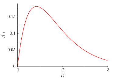
Figure 2: Graph of the numerical coefficient $A_{D}$ defined in Eq. (28) as a function of $D$ for $1\leq D\leq 3$.

In $D=3$ and $D=2$ we obtain $A_{3}=\frac{3}{160}\approx 0.0187$ and $A_{2}=\frac{\sqrt{3}}{16}\approx 0.108$, while $A_{D}\sim\frac{3\pi}{8}(D-1)\rightarrow 0$ for $D\rightarrow 1$. In three dimensions Eq. (27) agrees with the well-known Beliaev damping of the phonon mode in a Bose condensate Beliaev58 . Beliaev damping in $D=3$ and $D=2$ has recently been re-derived in Ref. Chung09 using Popov’s hydrodynamic approach; however, these authors did not integrate out the amplitude fluctuations, which renders the algebra more complicated than in our approach based on the effective action of phase fluctuations. The fact that for arbitrary $D>1$ Beliaev damping scales as $|\bm{k}|^{2D-1}$ has been pointed out previously by several authors Kreisel08 ; Sinner09 ; Zhitomirsky12 .

IV Phase fluctuations in one dimension

Obviously, Eq. (27) cannot be used to estimate the damping of phase fluctuations in one dimension, because the coefficient $A_{D}$ vanishes for $D\rightarrow 1$. The problem is that in the derivation of Eq. (27) we have inserted bare Green functions in the loop integration, which in $D=1$ is not accurate enough to obtain the damping of the phase fluctuations. A similar problem arises in the calculation of the damping of the excitations of a clean Luttinger liquid, which has been studied by Samokhin Samokhin98 by means of a self-consistent perturbative calculation taking the damping of intermediate states into account. Although in this case the spectral function is known to exhibit a non-Lorentzian line-shape with algebraic singularities Pustilnik06 , the overall width of the spectral function can be estimated correctly with this method.

Let us now use the method proposed by Samokhin Samokhin98 (see also Ref. Andreev80 ) to calculate the damping of phase fluctuations in the one-dimensional Bose gas. In fact, we shall go beyond Samokhin’s work and calculate the entire spectral line-shape of phase fluctuations. To include the damping of intermediate states in our perturbative self-energy (21), we replace the Gaussian propagators on the right-hand side by the exact propagators $G(K)$ of the phase mode, for which we use the spectral representation

$$G(k,i\omega)=\int_{-\infty}^{\infty}\frac{d\omega^{\prime}}{2\pi}\frac{B(k,\omega^{\prime})}{\omega^{\prime 2}+\omega^{2}},$$ (29)

where the spectral function

$$B(k,\omega)=2\omega{\rm Im}G(k,\omega+i\eta)$$ (30)

is real and positive. Retaining only the imaginary part of the self-energy, we find after analytic continuation that for frequencies close to $\pm E_{k}$ the spectral function can be approximated by

$$B(k,\omega)\approx\frac{u_{0}\gamma(k,\omega)}{(|\omega|-E_{k})^{2}+\gamma^{2}(k,\omega)}.$$ (31)

where the damping function $\gamma(k,\omega)$ satisfies the integral equation

$$\gamma(k,\omega) = \frac{{\rm sgn}\omega}{16m^{2}u_{0}}\int\frac{dk^{\prime}}{2\pi}\int_{0}^{|\omega|}d\omega^{\prime}B(k^{\prime},\omega^{\prime})$$ (32)

$$\times B(k-k^{\prime},\omega-\omega^{\prime})\biggr{\{}\frac{[{k}^{2}-{k}^{\prime 2}]^{2}}{|\omega|-\omega^{\prime}}$$

$$+\frac{[{k}^{2}-({k}-{k}^{\prime})^{2}]^{2}}{\omega^{\prime}}-\frac{[{k}^{\prime 2}-({k}-{k}^{\prime})^{2}]^{2}}{|\omega|}\biggl{\}}.$$

To solve this non-linear integral equation, we make the ansatz Samokhin98

$$\gamma(k,\omega)=\gamma_{k}f\left(\frac{|\omega|-E_{k}}{\gamma_{k}}\right),$$ (33)

where the on-shell damping is assumed to be of the form $\gamma_{k}=f_{0}|k|^{\alpha}$, with some exponent $\alpha$. The dimensionless function $f(z)$ is normalized such that $f(0)=1$, so that the dimensionful constant $f_{0}$ determines the strength of the on-shell damping. The function $f(z)$ is expected to be strongly peaked to $z=0$ and to decay as a power law for $|z|\gg 1$. After substituting the ansatz (33) into Eq. (32) we may scale out the $k$-dependence by introducing dimensionless integration variables $x=k^{\prime}/k$ and $y=(\omega^{\prime}-E_{k^{\prime}})/\gamma_{k^{\prime}}$. It is then easy to see that our ansatz is only consistent if $\alpha=2$. The constant $f_{0}$ is then given by

$$f_{0}=\frac{3\sqrt{I_{0}[f]}}{4m}\sqrt{\frac{k_{0}}{2\pi\rho}},$$ (34)

where the function $f(z)$ satisfies the integral equation

$$f(z)=\frac{I_{z}[f]}{I_{0}[f]},$$ (35)

with the non-linear functional $I_{z}[f]$ given by

$$I_{z}[f] = \int_{0}^{1}dx\frac{x}{1-x}\int_{-\infty}^{\infty}dy\frac{f(y)}{y^{2}+f^{2}(y)}$$ (36)

$$\times\frac{f\left(\frac{(z-y)x^{2}}{(1-x)^{2}}\right)}{\bigl{[}\frac{(z-y)x^{2}}{(1-x)^{2}}\bigr{]}^{2}+f^{2}\bigl{(}\frac{(z-y)x^{2}}{(1-x)^{2}}\bigr{)}}.$$

The integral equation (35) can easily be solved numerically. In practice we obtain convergence for any reasonable initial guess for the function $f(z)$. It turns out that the ansatz

$$f(z)\approx\frac{1}{1+f_{2}z^{2}}$$ (37)

with $f_{2}={\cal{O}}(1)$, does lead to a rather fast convergence after a few iterations. The solution of the integral equation (35) is represented by the solid line in Fig. 3.

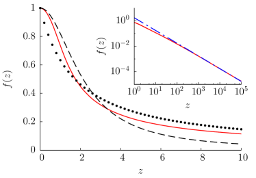
Figure 3: The solid line is the numerical solution of the integral equation (35). The dashed line represents the approximation (37) with $f_{2}=0.22$, which is reasonably accurate for $|z|\lesssim 5$. The dotted line represents the interpolation (38) with $f_{1}=0.58$. The logarithmic plot in the inset shows that for large $|z|$ the solution of the integral equation (35) vanishes as $1/|z|$. The dashed-dotted line in the inset is the curve $1/(0.58|z|)$.

In fact, for $f_{2}=0.22$ the ansatz (37) is already a reasonable approximation to the solution of Eq. (35) in the regime $|z|\lesssim 5$. Because the quadratic $z$-dependence of the exact solution for small $z$ is correctly described by Eq. (37), this ansatz describes the spectral function in the vicinity of the quasi-particle peaks quite accurately. On the other hand, as shown in the inset of Fig. 3, for large $|z|$ the numerical solution of Eq. (35) decays as $1/|z|$, which is not correctly described by our ansatz  (37). The tails of the spectral function are therefore better described by the interpolation formula

$$f(z)\approx\frac{1}{1+f_{1}|z|},$$ (38)

which for $f_{1}\approx 0.58$ has the correct asymptotics for large $|z|$, but is less accurate than Eq. (37) for small $z$.

Given our numerical solution $f(z)$ of the integral equation (35), we obtain

$$I_{0}[f]\approx 0.78,$$ (39)

and hence

$$f_{0}\approx\frac{0.66}{m}\sqrt{\frac{k_{0}}{2\pi\rho}}.$$ (40)

We conclude that for small wavevectors the on-shell damping of the phase mode in the one-dimensional Bose gas in units of its energy $E_{k}\approx c|k|$ can be written as

$$\frac{\gamma_{k}}{E_{k}}\approx 1.32\sqrt{\frac{k_{0}}{2\pi\rho}}\frac{|k|}{k_{0}}.$$ (41)

Note that the dimensionless ratio $k_{0}/2\pi\rho=mc/\pi\rho=u_{0}/\pi c$ can be identified with the Lieb-Liniger parameter divided by $\pi$. Keeping in mind that in the derivation of Eq. (41) we have neglected vertex corrections, we expect that the prefactor in Eq. (41) is accurate as long as the Lieb-Liniger parameter $u_{0}/c$ is small. Comparing Eq. (41) with the corresponding expression (27) in $D>1$ we see that in one dimension the damping involves an additional factor of $|k|/k_{0}$; however, in $D=1$ the prefactor is proportional to the square root of the Lieb-Liniger parameter $u_{0}/c$, whereas in $D>1$ it is linear in the corresponding dimensionless parameter $k_{0}^{D}/2\pi\rho$.

Since the solution of the integral equation (35) gives the entire scaling function $f(z)$ in Eq. (33), it is now easy to obtain the momentum- and frequency dependent spectral function $B(k,\omega)$ of phase fluctuations of the one-dimensional Bose gas. The result is plotted in Fig. 4.

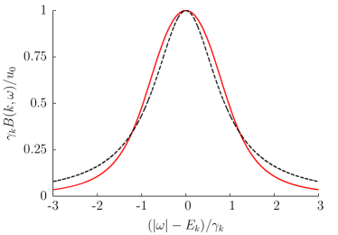
Figure 4: Normalized spectral function $\gamma_{k}B(k,\omega)/u_{0}$ of phase fluctuations of the one-dimensional Bose gas as a function of frequency for fixed $k=0.5\,k_{0}$ and Lieb-Liniger parameter $u_{0}/c=0.1$. The on-shell damping is in this case $\gamma_{k}/(ck_{0})=0.059$. The dashed line represents a fit to a Lorentzian with on-shell damping $\gamma_{k}$.

Obviously, for frequencies not too far away from the central peak ($||\omega|-E_{k}|\lesssim 2\gamma_{k}$) the line-shape can be approximated by a Lorentzian, but outside this regime the spectral function decays faster. Using the fact that $f(z)\sim(f_{1}|z|)^{-1}$ for large $z$ we find that the tails of the spectral function are

$$B(k,\omega)\sim\frac{u_{0}\gamma(k,\omega)}{(|\omega|-E_{k})^{2}}\sim\frac{1}{f_{1}}\frac{u_{0}\gamma_{k}^{2}}{||\omega|-E_{k}|^{3}},$$ (42)

which decays faster than a Lorentzian by a factor of $\gamma_{k}/||\omega|-E_{k}|$. Note that our ansatz (33) is only justified for $\left|\left|\omega\right|-E_{k}\right|\lesssim E_{k}$ so that the result (42) does not describe the asymptotics for $\left|\omega\right|\rightarrow\infty$.

V Summary and Conclusions

In summary, we have derived an effective action describing the dynamics of low-energy and long-wavelength phase fluctuations of superfluid bosons. Using this action, we have then calculated the leading momentum dependence of the damping of the phase fluctuations in arbitrary dimensions. For $D>1$ a simple perturbative calculation yields the usual Beliaev damping, which scales as $|{\bm{k}}|^{2D-1}$ in $D$ dimensions. For $D\rightarrow 1$ the prefactor of $|{\bm{k}}|^{2D-1}$ vanishes, and the damping is proportional to $k^{2}$. We have obtained this result by taking the damping of the intermediate states in the loop integration self-consistently into account. In one dimension, we have also calculated the spectral function of phase fluctuations, which has a Lorentzian line-shape for frequencies close to the quasi-particle peaks associated with the sound mode, but for larger deviations from the peaks decays faster than a Lorentzian.

Since the vertices of the effective action for the phase fluctuations vanish for zero wavevectors or frequencies, we believe that higher orders in perturbation theory do not qualitatively modify our results. In particular, in one dimension the spectral function of phase fluctuations does not contain any algebraic singularity, in contrast to the spectral function of the amplitude fluctuations Khodas07 ; Pustilnik06 . We are not aware of experimental methods to directly measure the spectral function of phase fluctuations, so that we cannot compare our result for the spectral line-shape with experiments. However, for non-perturbative calculations of the single-particle Greens function of superfluid bosons one usually assumes that the Gaussian approximation is sufficient to calculate the propagator of the phase fluctuations Popov83 ; Khodas07 . Our results imply that the Gaussian approximation is indeed well justified in this case, because the damping of the phase mode is small, so that in the superfluid state the phase fluctuations can propagate as well-defined quasi-particles, even in one dimension.

References

- (1) S. T. Beliaev, Zh. Eksp. Teor. Fiz. 34, 417 (1958), ibid. 433 (1958) [Sov. Phys. JETP 7, 289 (1958); ibid. 7, 299 (1958)].
- (2) J. Gavoret and P. Nozières, Ann. Phys. 28, 349 (1964).
- (3) H. Shi and A. Griffin, Phys. Rep. 304, 1 (1998).
- (4) J. O. Andersen, Rev. Mod. Phys. 76, 599 (2004).
- (5) N. N. Bogoliubov, Izv. Akad. Nauk SSSR, Ser. Fiz. 11, 77 (1947) [J. Phys. (Moscow) 11, 23 (1947)].
- (6) A. A. Nepomnyashchy and Yu. A. Nepomnyashchy, Pis’ma Zh. Eksp. Teor. Fiz. 21, 3 (1975) [JETP Lett. 21, 1 (1975)], and Zh. Eksp. Teor. Fiz. 75, 976 (1978) [Sov. Phys. JETP 48, 493 (1978)]; Yu. A. Nepomnyashchy, Zh. Eksp. Teor. Fiz. 85 1244 (1983) [Sov. Phys. JETP 58, 722 (1983)].
- (7) N. Dupuis, Phys. Rev. E 83, 031120 (2011).
- (8) C. Castellani, C. Di Castro, F. Pistolesi, and G. C. Strinati, Phys. Rev. Lett. 78, 1612 (1997); F. Pistolesi, C. Castellani, C. Di Castro, and G. C. Strinati, Phys. Rev. B 69, 024513 (2004).
- (9) A. Sinner, N. Hasselmann, and P. Kopietz, Phys. Rev. Lett. 102, 120601 (2009); Phys. Rev. A 82, 063632 (2010).
- (10) N. Dupuis, Phys. Rev. Lett. 102, 190401 (2009); Phys. Rev. A 80, 043627 (2009).
- (11) V. N. Popov, Teor. Mat. Fiz. 11, 354 (1972) [Theor. Math. Phys. 11, 565 (1972)].
- (12) V. N. Popov, Functional Integrals in Quantum Field Theory and Statistical Physics, (Kluwer, Dordrecht, 1983).
- (13) In three dimensions can be identified with the bare interaction in the weak coupling limit. In reduced dimensions, represents an effective coupling constant, taking the embedding of the system into a confining potential into account, as explained by M. Olshanii, Phys. Rev. Lett. 81, 938 (1998).
- (14) V. N. Popov, Teor. Mat. Fiz. 30, 346 (1977) [Theor. Math. Phys. 30, 222 (1977)].
- (15) E. H. Lieb and W. Liniger, Phys. Rev. 130, 1605 (1963); E. H. Lieb, Phys. Rev. 130 1616 (1963).
- (16) M. Khodas, M. Pustilnik, A. Kamenev, and L. I. Glazman, Phys. Rev. Lett. 99, 110405 (2007).
- (17) A. Imambekov and L. I. Glazman, Phys. Rev. Lett. 100, 206805 (2008).
- (18) A. Kreisel, F. Sauli, N. Hasselmann, and P. Kopietz, Phys. Rev. B 78, 035127 (2008).
- (19) M. E. Zhitomirsky and A. L. Chernyshev, arXiv:1205.5278v1 [cond-mat.str-el] (2012).
- (20) M.-C. Chung and A. Bhattacherjee, New J. Phys. 11, 123012 (2009).
- (21) K. V. Samokhin, J. Phys.: Condens. Matter 10, L533 (1998).
- (22) A. F. Andreev, Zh. Eksp. Teor. Fiz. 78, 2064 (1980) [Sov. Phys. JETP 51, 1038 (1980)].
- (23) M. Pustilnik, M. Khodas, A. Kamenev, and L. I. Glazman, Phys. Rev. Lett. 96, 196405 (2006).