Endstates in multichannel spinless $p$-wave superconducting wires

Abstract

Multimode spinless $p$-wave superconducting wires with a width $W$ much smaller than the superconducting coherence length $\xi$ are known to have multiple low-energy subgap states localized near the wire’s ends. Here we compare the typical energies of such endstates for various terminations of the wire: A superconducting wire coupled to a normal-metal stub, a weakly disordered superconductor wire, and a wire with smooth confinement. Depending on the termination, we find that the energies of the subgap states can be higher or lower than for the case of a rectangular wire with hard-wall boundaries.

I Introduction

In the current search for Majorana fermions in nano-wire geometries Beenakker2011 ; Alicea2012 an important theoretical challenge is to understand the multiplicity of possible fermionic bound states that can form at the ends of the wire and how a possible Majorana bound state can be identified among them. This is particularly relevant for multichannel geometries, in which fermionic states localized near the ends of the wire are expected to occur at energies much smaller than the excitation gap for bulk excitations if the wire width is much smaller than the superconducting coherence length. In this article we explore the dependence of these sub-gap end-states on the details of the termination of the wire and on impurity scattering.

The interest in isolating Majorana fermions arises because their non-local properties and non-abelian braiding statistics render them potentially useful for fault tolerant quantum computation.kitaev2003 ; freedman1998 ; Read2000 ; Ivanov2001 ; Kitaev2006 ; Nayak2008 ; Wilczek2009 Majorana fermions occur — at least theoretically — at the ends of one-dimensional spinless $p$-wave superconductors.Kitaev2001 Recent proposals suggest ways of engineering solid-state systems that effectively behave as spinless $p$-wave superconductors by combining an s-wave superconductor and a topological insulator,Fu2008 ; Cook2011 a semiconductor Sau2010 ; Alicea2010 ; Oreg2010 ; Lutchyn2010 or ferromagnet.Duckheim2011 ; Chung2011 ; Choy2011 ; Martin2012 ; Kjaergaard2012 Building on the proposals of Refs. Oreg2010, ; Lutchyn2010, , two experimental groups have reported an enhanced tunneling density of states at the ends of InAs and InSb wires in proximity to a superconductor, consistent with the existence of Majorana bound states at the ends of these wires,Mourik2012 ; Das2012 whereas a number of other groups claim the observation of Majorana bound states using different methods.Williams2012 ; Rokhinson2012 ; Deng2012

Whereas the original proposals for Majorana fermions in wire geometries focused on one-dimensional systems, it is by now well established that the topological superconducting phase with Majorana end states may persist in a quasi-one-dimensional multichannel setting.Wimmer2010 ; Potter2010 ; Lutchyn2011 ; Potter2011 ; Stanescu2011 ; Zhou2011 ; Kells2012 ; Potter2012 ; Lim2012 ; Gibertini2012 ; Tewari2012 A difference between the quasi-one-dimensional and one-dimensional settings is, however, that a possible zero-energy Majorana state localized at the wire’s end may co-exist with other fermionic sub-gap states, analogous to those found in vortex cores of bulk superconductors.Caroli1964 For the case of an $N$-channel spinless $p+ip$ superconductor with a rectangular geometry and with width $W$ much smaller than the superconducting coherence length $\xi$, three of us recently showed that the number of such fermionic subgap states is $\sim N/2$, and that their typical energy is $\varepsilon_{\rm typ}\sim\Delta(W/\xi)^{2}$, $\Delta$ being the superconducting gap size.Kells2012 The lowest-lying and highest-lying fermionic subgap states have energies $\varepsilon_{\rm min}\sim\varepsilon_{\rm typ}/N\ln N$ and $\varepsilon_{\rm max}\sim N\varepsilon_{\rm typ}$, respectively. The fermionic subgap states also exist in a non-topological phase without zero-energy Majorana end-state, thus posing a potential obstacle for the identification of the topological phase through the observation of an enhanced density of states near zero energy.

In a recent article, Potter and LeePotter2012 observe that the dependence of the energy of the lowest-lying fermionic subgap state on system parameters changes qualitatively if the rectangular geometry of Ref. Kells2012, is replaced by a geometry with rounded ends. They point out that the calculation of the energy of the fermionic subgap state for the rectangular geometry is plagued by a subtle cancellation, which does not appear for a generic wire ending. In particular it was found in Ref. Potter2012, that the lowest-lying fermionic subgap state has an energy significantly above the prediction of Ref. Kells2012, for a wire with width $W\sim\xi$ and rounded ends.

Motivated by these observations we present here a detailed investigation of the effect that the wire termination has on the energies of the fermionic subgap states for the multichannel spinless $p+ip$ superconductor. Remarkably, we find that, depending on the details of the wire ending, the energies of the fermionic subgap states can be significantly above, as well as below the rectangular-wire case of Ref. Kells2012, . We find an increase of the energies of the subgap states if an arbitrarily-shaped normal layer is attached to the wire’s end, the magnitude of the increase being consistent with the estimate of Ref. Potter2012, for a wire with rounded ends. On the other hand, the presence of impurities — weak enough to preserve the topological phase Motrunich2001 ; Brouwer2011b — on average reduces the energies of the fermionic end states below the estimate of Ref. Kells2012, , while a smooth confinement (with a slowly increasing potential energy providing the confinement along the wire’s axis) leads to even smaller energies of the fermionic subgap states.

Our results are derived for the two-dimensional spinless $p+ip$ superconducting strip of width $W$. The model of a spinless $p+ip$ superconductor is an effective low-energy description for the various proposals to realize one-dimensional or quasi-one-dimensional topological superconductors, provided the number $N$ of propagating channels at the Fermi level is chosen equal to the number of spinless (i.e., helical or spin-polarized) channels in the case of the semiconductor or ferromagnet proposals. (The edges of a topological insulator always have $N=1$, so that a multichannel $p+ip$ model is not relevant in that case.) A mapping between the spinless $p$-wave model and the semiconductor-wire proposals is given in the appendix.

The remainder of this article is organized as follows: In Sec. II we briefly review the symmetries of the model (2) and the reason for the appearance of multiple low-lying states if the wire width $W$ is much smaller than the superconducting coherence length $\xi$. In Sec. III we describe a scattering theory of fermionic subgap states with arbitrary wire endings. Section IV discusses the $p+ip$ model with weak disorder, while the effect of a smooth potential at the wire’s end is discussed in Sec. V. We conclude in Sec. VI.

II $p+ip$ model

Our calculations are performed for a two-dimensional spinless $p+ip$ superconductor, which is described by the two-component Bogoliubov-de Gennes Hamiltonian, which we write as

$$H=H_{0}+H_{y}+H_{V},$$ (1)

with

$$H_{0} = \left(\frac{p^{2}}{2m}-\mu\right)\tau_{z}+\Delta^{\prime}p_{x}\tau_{x},$$

$$H_{y} = -\Delta^{\prime}p_{y}\tau_{y},$$

$$H_{V} = V({\boldsymbol{r}})\tau_{z}.$$ (2)

Here $\tau_{x}$, $\tau_{y}$, and $\tau_{z}$ are Pauli matrices in particle-hole space, $\Delta^{\prime}$ specifies the $p$-wave superconducting order parameter, $\mu=\hbar^{2}k_{\rm F}^{2}/2m$ and $m$ are the chemical potential and electron mass, and $V({\boldsymbol{r}})$ a potential that describes the confinement at the ends of the wire as well as the scattering off impurities. The two-dimensional coordinate ${\boldsymbol{r}}=(x,y)$, where $0<y<W$, with hard-wall boundary conditions at $y=0$ and $y=W$. The superconducting order parameter derives from proximity coupling to a bulk superconductor, so that no self-consistency condition for $\Delta^{\prime}$ needs to be employed.

Hypothetical end states are localized within a distance of the order of the superconducting coherence length $\xi=\hbar(\Delta^{\prime}m)^{-1}$ from the wire’s ends. For thin wires with $W\ll\xi$ it is a good starting point to analyze the Hamiltonian $H=H_{0}+H_{V}$ without the term $H_{y}$. The Hamiltonian $H_{0}$ has a chiral symmetry,Tewari2011 $\tau_{y}H_{0}\tau_{y}=-H_{0}$, and there exist

$$N=\mbox{int}\,[(W/\pi)\sqrt{k_{\rm F}^{2}-\xi^{-2}}]$$ (3)

Majorana bound states at each end of the wire. Kells2012 ; Potter2012 ; Gibertini2012 ; Tewari2012 The stepwise increase of the number of Majorana end states for wire widths $W$ such that $(W/\pi)\sqrt{k_{\rm F}^{2}-\xi^{-2}}$ is an integer is accompanied by a closing of the bulk excitation gap of $H_{0}$. Inclusion of the potential term $H_{V}$ does not lift the degeneracy of the Majorana end states, since $H_{V}$ preserves the chiral symmetry, although it may change the boundaries of the phases with different $N$ if $H_{V}$ is nonzero in the bulk of the wire. In contrast, the term $H_{y}$ breaks the chiral symmetry and couples the $N$ Majorana bound states, giving rise to (generically) $\mbox{int}\,(N/2)$ fermionic states at each end and a single Majorana end state if $N$ is odd. If $W\ll\xi$ the splitting of the end states is small in comparison to the bulk energy gap $\Delta=\Delta^{\prime}\hbar k_{F}$, and the resulting fermionic states cluster near zero energy.Kells2012 ; Potter2012

A schematic picture of the end-state spectrum as a function of $W$ is shown in Fig. 1. The end states are characterized by the energy $\varepsilon_{\rm min}$ of the lowest-lying fermionic end state, the typical end-state energy $\varepsilon_{\rm typ}$, and the energy $\varepsilon_{\rm max}$ of the highest-lying end state. For small $N$ these three energy scales are comparable, but for large $N$ they may differ considerably. The energy $\varepsilon_{\rm min}$ serves as the “energy gap” protecting the topological state and sets the required energy resolution if the presence or absence of a Majorana end state is detected through a tunneling density of states measurement.

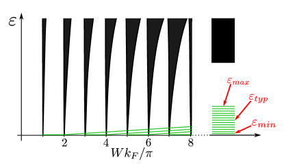
Figure 1: (Color online) Schematic picture of the spectrum of low-energy excitations of the a $p+ip$ wire as a function of its width $W$. The gap for bulk excitations closes at those values of $W$ for which $(W/\pi)\sqrt{k_{\rm F}^{2}-\xi^{-2}}$ is an integer. When the bulk gap is finite, there are low-energy subgap states localized near the ends of the wire. In the text, we use $\varepsilon_{\rm min}$ to denote the energy of the lowest-lying fermionic subgap state, $\varepsilon_{\rm typ}$ for the typical energy of a subgap state, and $\varepsilon_{\rm max}$ for the energy of the highest-lying fermionic subgap state.

The specific case of a rectangular wire geometry, with hard-wall boundary conditions at each end of the wire and without disorder, was investigated in Ref. Kells2012, . We now investigate two other possible terminations, as well as the effect of disorder on the energies of subgap endstates in multichannel spinless $p$-wave superconducting wires.

III Normal-metal stub

In this section, we consider a quasi-one-dimensional spinless $p+ip$ superconductor without disorder and coupled to a normal-metal stub at its end. We choose coordinates, such that the spinless superconductor occupies the space $x>0$, $0<y<W$, see Fig. 2. Such a wire ending is relevant, e.g., for the experimental geometry of Ref. Mourik2012, , in which a topological phase is induced in a semiconductor nanowire by laterally coupling it to a superconductor, while a part of the wire sticks out from under the superconductor and is pinched off by a gate at a finite distance.

We take the Hamiltonian of the normal stub to be real and symmetric, in order to preserve the chiral symmetry of the Hamiltonian $H_{0}$. Following Ref. Kells2012, we first solve for the wavefunctions $\psi^{(j)}$ of the $N$ Majorana modes for the Hamiltonian $H_{0}$ and then treat $H_{y}$ in perturbation theory. The potential term $H_{V}$ is set to zero throughout this calculation.

The Majorana states have support in the normal stub as well as in a segment of the superconducting wire of length $\sim\xi$. In the superconducting region $x>0$ the wavefunctions $\psi$ of the Majorana states can be written as

$$\psi({\boldsymbol{r}}) = \sum_{n}a_{n-}\phi_{n-}({\boldsymbol{r}})+a_{n+}\phi_{n+}({\boldsymbol{r}}),$$ (4)

where the basis states $\phi_{n\pm}$, $n=1,2,\ldots,N$, read

$$\phi_{n\pm}({\boldsymbol{r}}) = \left(\begin{array}[]{c}e^{i\pi/4}\\ e^{-i\pi/4}\end{array}\right)\sqrt{\frac{2m}{W\hbar k_{n}}}e^{\pm ik_{n}x-x/\xi}\sin\left(\frac{n\pi y}{W}\right),$$ (7)

with

$$k_{n}=\sqrt{k_{\rm F}^{2}-(n\pi/W)^{2}}.$$ (9)

The basis states $\phi_{n\pm}$ have been normalized to unit flux. The above expressions for the basis states and their normalization are valid up to corrections of order $(W/\xi)^{2}$, which we neglect throughout this calculation.

The coupling to the normal-metal stub imposes boundary conditions on the coefficients $a_{n\pm}$, which we express in terms of the scattering matrix $S_{nn^{\prime}}$ of the normal stub,

$$a_{n+}=\sum_{n^{\prime}}S_{nn^{\prime}}a_{n^{\prime}-},\ \ a_{n-}=\sum_{n^{\prime}}S_{nn^{\prime}}^{*}a_{n^{\prime}+},$$ (10)

Because the Hamiltonian of the normal stub is real and symmetric, the scattering matrix $S_{nn^{\prime}}$ is unitary and symmetric, $S_{nn^{\prime}}=S_{n^{\prime}n}$, which ensures that the $2N$ equations (10) have $N$ independent solutions, corresponding to the $N$ Majorana end states.

For finding an explicit representation of the $N$ Majorana states $\psi^{(j)}$, $j=1,2,\ldots,N$ we use the fact that the scattering matrix $S$ and the Wigner-Smith time-delay matrixWigner1955 ; Smith1960 $Q=i\hbar S^{\dagger}\partial S/\partial\mu$ of the normal stub can be simultaneously decomposed as

$$S=U^{\rm T}U,\ \ Q=U^{\dagger}\mbox{diag}\,(\tau_{1},\ldots,\tau_{N})U,$$ (11)

where $U$ is an $N\times N$ unitary matrix and the $\tau_{i}>0$, $i=1,2,\ldots,N$, are the so-called “proper time delays”. With this decomposition, a solution to the boundary conditions (10) is given by

$$a_{n+}^{(j)}=U_{nj},\ \ a_{n-}^{(j)}=U_{nj}^{*},\ \ j=1,2,\ldots,N.$$ (12)

The $N$ states that are defined through these coefficients,

$$\tilde{\psi}^{(j)}({\boldsymbol{r}}) = \sum_{n}a_{n-}^{(j)}\phi_{n-}({\boldsymbol{r}})+a_{n+}^{(j)}\phi_{n+}({\boldsymbol{r}}),$$ (13)

are Majorana modes (they satisfy $\tilde{\psi}^{(j)*}=\tau_{x}\tilde{\psi}^{(j)}$), but they are not necessarily orthonormal. In order to construct an orthonormal set, we first calculate the scalar product $M_{jl}$ of the modes $\tilde{\psi}^{(j)}$,

$$M_{jl} = \int_{0}^{\infty}dx\int_{0}^{W}dy\,\tilde{\psi}^{\ast(j)}({\boldsymbol{r}})\tilde{\psi}^{(l)}({\boldsymbol{r}})$$

$$\mbox{}+\int_{\text{stub}}d\textbf{r}\tilde{\psi}^{\ast(j)}({\boldsymbol{r}})\tilde{\psi}^{(l)}({\boldsymbol{r}})$$

$$= \sum\limits_{n}\frac{2m\xi}{\hbar k_{n}}\mbox{Re}\,\left(U_{nj}U^{*}_{nl}+\frac{U_{nj}U^{*}_{nl}}{1-ik_{n}\xi}\right)+2\tau_{j}\delta_{jl},$$

Here we used the relation between the Wigner-Smith time delay matrix and the normalization of scattering states in order to perform the integration over the sub, see Ref. Smith1960, . The overlap matrix $M$ is real, positive definite, and symmetric. It is manifestly diagonal if the scattering matrix $S$ and the time-delay matrix $Q$ are diagonal or in the “large-stub limit”, which is defined as the limit in which the mean inverse dwell time $\hbar/\bar{\tau}$ is much smaller than the superconducting gap. In both cases, one obtains an orthonormal basis for the $N$ Majorana modes by setting $\psi^{(j)}=\tilde{\psi}^{(j)}/\sqrt{M_{jj}}$. In the general case, $M$ is not diagonal, however, and one has to construct an orthonormal system with the help of the orthogonal transformation $O$ that diagonalizes $M$, i.e., $O^{T}MO=\lambda^{2}$, where $\lambda=\mbox{diag}\,(\lambda_{1},\lambda_{2},\ldots,\lambda_{N})$ is a diagonal matrix with positive elements. The corresponding orthonormal basis set one thus obtains reads

$$\psi^{(j)}({\boldsymbol{r}})=\sum_{n=1}^{N}\tilde{\psi}^{(n)}({\boldsymbol{r}})O_{nj}\lambda_{n}^{-1}.$$ (15)

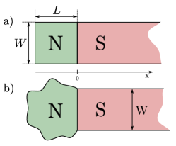
Figure 2: (Color online) Schematic drawing of a spinless $p$-wave superconducting wire (S) coupled to a normal-metal (N) stub at one end. The top panel shows a rectangular stub, the bottom panel shows a chaotic cavity attached to the superconducting wire.

Inclusion of $H_{y}$, which breaks the chiral symmetry, gives rise to a splitting of the $N$ degenerate Majorana end states constructed above. With respect to the unnormalized states $\tilde{\psi}^{(j)}$, this splitting is described by the $N\times N$ matrix

$$\tilde{H}^{\text{(1)}}_{jl} = \langle\tilde{\psi}^{(j)}|H_{y}|\tilde{\psi}^{(l)}\rangle$$ (16)

$$= \frac{4i\Delta^{\prime}m}{W}\sum\limits_{nn^{\prime}}\frac{nn^{\prime}[1-(-1)^{n+n^{\prime}}]}{(n^{\prime 2}-n^{2})\sqrt{k_{n}k_{n^{\prime}}}}$$

$$\mbox{}\times\sum_{\pm}\left[\textrm{Im}\,\frac{U_{nj}U^{*}_{n^{\prime}l}}{k_{n^{\prime}}\pm k_{n}}+\frac{2}{\xi}\textrm{Re}\,\frac{U_{nj}U^{*}_{n^{\prime}l}}{(k_{n^{\prime}}\pm k_{n})^{2}}\right],$$

where we neglected corrections smaller by a factor of order $(W/\xi)^{2}$. The matrix $\tilde{H}^{\rm(1)}_{jl}$ is antisymmetric and purely imaginary, which ensures the existence of a single zero-energy bound state if $N$ is odd. In order to find a true effective Hamiltonian $H^{\rm(1)}$, the eigenvalues of which represent the energies of the fermionic end states, one should transform to the basis of orthogonal states $\psi^{(j)}$ introduced in Eq. (15),

$$H^{\rm(1)}=\frac{1}{\lambda}O^{T}\tilde{H}^{\rm(1)}O\frac{1}{\lambda}.$$ (17)

In the special case $N=2$, this transformation can be carried out for an arbitrary scattering matrix $S$ and the energy of the resulting single fermionic bound state is

$$\varepsilon=\frac{|\tilde{H}^{\rm(1)}_{12}|}{\sqrt{M_{11}M_{22}-M_{12}^{2}}}.$$ (18)

We now discuss two particular realizations of a metal stub in detail.

III.1 Rectangular stub

First, we consider a rectangular stub of length $L$ attached to the spinless $p$-wave superconducting wire, see Fig. 2a. For this geometry, both the scattering matrix $S$ and the Wigner-Smith time-delay matrix $Q$ are diagonal,

$$S_{nn^{\prime}}=-e^{2ik_{n}L}\delta_{nn^{\prime}},\ \ Q_{nn^{\prime}}=\frac{2mL}{\hbar k_{n}}\delta_{nn^{\prime}},$$ (19)

with $k_{n}$ given by Eq. (9). Since there is no mixing between different channels, the zero energy modes $\tilde{\psi}^{(j)}$ already form an orthogonal basis. The effective Hamiltonian in the normalized basis $\psi^{(j)}=\tilde{\psi}^{(j)}/\sqrt{M_{jj}}$ has $H^{\rm(1)}_{jl}=0$ if $j+l$ is even and

$$H^{\rm(1)}_{jl} = \frac{4i\Delta_{y}\hbar jl}{W(\xi+2L)(l^{2}-j^{2})}\sum_{\pm}\left\{\frac{\sin[L(k_{j}\pm k_{l})]}{k_{l}\pm k_{j}}\right.$$ (20)

$$\left.\mbox{}+\frac{2W}{\pi\xi}\frac{\cos[L(k_{j}\pm k_{l})]}{(k_{l}\pm k_{j})^{2}}\right\}$$

if $j+l$ is odd, up to corrections smaller by a factor of order $(W/\xi)^{2}$.

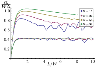
Figure 3: (Color online) Typical and maximal energies of fermionic subgap states in a spinless $p$-wave superconductor with a rectangular normal-metal stub of length $L$ as a function of $L/W$ for different channels numbers ($N=15,\,27,\,55,\,99$). The maximal energies $\varepsilon_{\rm max}$ have a finite-$N$ correction of order $\varepsilon_{\rm m}/\sqrt{N}$, which is why the curves for $\varepsilon_{\rm max}$ still show an $N$ dependence for large $N$.

The second term in the effective Hamiltonian (20) is smaller than the first one by a factor of order $W/\xi$. However, only this second term contributes in the limit $L=0$ in which there is no normal metal stub.Kells2012 This is a variation of the cancellation effect pointed out by Potter and Lee.Potter2012 We now analyze the eigenvalues of the effective Hamiltonian $H^{\rm(1)}$ for finite $L$, when the first term between brackets dominates.

Since no closed-form expressions for the eigenvalues of $H^{\rm(1)}$ could be obtained, we numerically diagonalized $H^{\rm(1)}$ and investigated the dependence of the minimum, typical, and maximal positive eigenvalues on the ratio $L/W$ as well as the channel number $N$. For $L\sim W$, this analysis gives

$$\varepsilon_{\rm typ}\sim\varepsilon_{\rm m}\equiv\frac{W\Delta}{\xi},$$ (21)

see Fig. 3. The maximum and minimum energies of the subgap states scale as $\varepsilon_{\rm min}\sim\varepsilon_{\rm typ}/N$, $\varepsilon_{\rm max}\sim\varepsilon_{\rm typ}$. A similar analysis for $k_{\rm F}^{-1}\ll L\ll W$ gives estimates for $\varepsilon_{\rm min}$, $\varepsilon_{\rm typ}$, and $\varepsilon_{\rm max}$ which are smaller by a factor $L/W$, whereas for $L\ll k_{\rm F}^{-1}$, they are smaller by a factor $L^{3}k_{\rm F}^{2}/W$. A crossover to the results of Ref. Kells2012, takes place for $L\lesssim(W^{2}/k_{\rm F}^{2}\xi)^{1/3}$. In the limit of large $N$ the energies of the fermionic subgap states are best described through their level density, which is shown in Fig. 4.

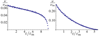
Figure 4: (Color online) Level density of fermionic subgap states for a rectangular stub in the limit of large $N$, for $L/W=0.1$ (left) and $L/W=3$ (right). The level density is measured in units of $\nu_{\rm m}=N/\varepsilon_{\rm m}$.

III.2 Chaotic Cavity

As a second example, we consider a chaotic cavity attached to the end of the superconducting wire, see Fig. 2b. In this case, the unitary matrix $U$ is randomly distributed in the unitary group,Beenakker1997 whereas the proper delay times have the probability distribution Brouwer1997

$$P(\tau_{1},...,\tau_{N}) \propto \prod_{j=1}^{N}\theta(\tau_{j})\tau_{j}^{-3N/2-1}e^{-N\bar{\tau}/2\tau_{j}}$$ (22)

$$\mbox{}\times\prod_{i<j}|\tau_{i}-\tau_{j}|,$$

with the average delay time $\bar{\tau}$. In this case, the matrix $U$ is not diagonal, and the prescription of Eq. (17) needs to be used in order to construct the effective Hamiltonian $H^{\rm(1)}$ for the low-energy subgap states. As in the previous case, we could not obtain closed-form expressions for the energies of the fermionic subgap states and had to resort to a numerical analysis, in which the unitary matrices $U$ were generated according to the Haar measure on the unitary group and the time-delays $\tau_{i}$ according to the probability distribution given above, following the method described in Ref. Cremers2002, . This analysis gives different results for the limiting cases of a “small cavity” and a “large cavity”, corresponding to the inverse mean dwell time $\hbar/\bar{\tau}$ large or small in comparison to the superconducting gap $\Delta$.

Small-cavity limit. In the small-cavity limit, the normalization of the $N$ Majorana states $\psi^{(j)}$ is dominated by the integration over the superconducting wire. Not counting the Majorana states, the excitation spectrum of the cavity has a gap comparable to the bulk excitation gap $\Delta$. Upon including $H_{y}$ one obtains $N$ fermionic subgap states, which have a typical energy

$$\varepsilon_{\rm typ}\sim\varepsilon_{\rm s}\equiv\frac{W\Delta}{\xi},$$ (23)

and $\varepsilon_{\rm max}\sim\varepsilon_{\rm typ}$, $\varepsilon_{\rm min}\sim\varepsilon_{\rm typ}/N$. The precise location of the subgap states depends on the precise scattering matrix of the cavity. The mean level density for an ensemble of cavities is shown in the left panel Fig. 5.

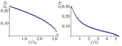
Figure 5: (Color online) Level density of fermionic subgap states in the small-cavity limit (left) and large-cavity limit (right). The level density is measured in units of $\nu_{\rm s}=N/\varepsilon_{\rm s}$ and $\nu_{\rm l}=N/\varepsilon_{\rm l}$ for the left and right panels, respectively.

Large-cavity limit. In the large-cavity limit, the overlap matrix $M_{jl}$ is dominated by the in-cavity parts of the wavefunctions, so that the Majorana modes $\tilde{\psi}^{(j)}$ are already orthogonal and the effective Hamiltonian $H_{jl}^{\rm(1)}=\tilde{H}_{jl}^{\rm(1)}/\sqrt{4\tau_{j}\tau_{l}}$, with $\tilde{H}_{jl}^{\rm(1)}$ given in Eq. (16). Not counting the Majorana states, the cavity’s excitation spectrum has a gap of order $E_{\rm T}=\hbar/\pi\bar{\tau}$,Melsen1997 where $\bar{\tau}$ is the mean dwell time in the cavity. In this case, the typical energy of the fermionic subgap states is

$$\epsilon_{\rm typ} \sim \varepsilon_{\rm l}\equiv\frac{E_{\rm T}W}{\xi},$$ (24)

while $\varepsilon_{\rm max}\sim\varepsilon_{\rm typ}$ and $\varepsilon_{\rm min}\sim\varepsilon_{\rm typ}/N$. The mean level density of the subgap states for an ensemble of cavities is shown in the right panel of Fig. 5.

IV $p+ip$ model with disorder

Whereas strong disorder is known to destroy the topological superconducting phase in the $p+ip$ model in one dimension, weak disorder with mean free path $l>\xi/2$ preserves the topological phase.Motrunich2001 ; Brouwer2011b In this section we investigate the effect of weak disorder on the energies of the fermionic subgap states in a multichannel rectangular $p+ip$ model. Because the disorder is necessarily weak (strong disorder suppresses the topological phase), the effect of disorder can be treated in perturbation theory.

Starting point of our analysis is the chiral-symmetric Hamiltonian $H_{0}$, which has $N$ normalized Majorana bound states $|\,\psi^{(j)}\rangle$, $j=1,2,\ldots,N$ at each end of the wire. We take a rectangular geometry, with a wire end and hard-wall boundary conditions at $x=0$, and take the potential $V({\boldsymbol{r}})$ to be a Gaussian white noise potential with mean $\langle V({\boldsymbol{r}})\rangle=0$ and variance

$$\langle V({\boldsymbol{r}})V({\boldsymbol{r}}^{\prime})\rangle=\frac{v_{\rm F}^{2}}{k_{\rm F}l}\delta({\boldsymbol{r}}-{\boldsymbol{r}}^{\prime}),$$ (25)

where $l$ is the mean free path and $v_{\rm F}=\hbar k_{\rm F}/m$ the Fermi velocity. In our perturbative analysis we treat both the impurity potential $V$ and the transverse superconducting order as perturbations and write

$$H=H_{0}+U,$$ (26)

where $U=H_{y}+H_{V}$ contains the superconducting correlations coupling to $p_{y}$ as well as the impurity potential.

The effective Hamiltonian $H_{\rm eff}$ describing the splitting of the $N$ Majorana states into fermionic subgap states can be found using the degenerate perturbation theory of Kato Kato1949 and Bloch.Bloch1958 (For additional details on this methodology see also Refs. Messiah1961, and Jordan2008, .) Defining $P=\sum|\,\psi^{(j)}\rangle\langle\psi^{(j)}\,|$ as the projector onto the zero-energy subspace and $Q=1-P$, we can then write using Bloch’s method

$$H_{\rm eff} = PUP-PU\frac{Q}{H_{0}}UP+PU\frac{Q}{H_{0}}U\frac{Q}{H_{0}}UP$$ (27)

$$\mbox{}-\frac{1}{2}\left(PU\frac{Q}{H_{0}^{2}}UPUP+PUPU\frac{Q}{H_{0}^{2}}UP\right).$$

It is essential to note that the disorder potential $V({\boldsymbol{r}})$ alone cannot lift the degeneracy of the Majorana end states at any order of the perturbation theory. This can be understood directly from the observation that the disorder potential $V({\boldsymbol{r}})$ does not break the chiral symmetry of the unperturbed Hamiltonian $H_{0}$ that is responsible for the $N$-fold degeneracy. On the level of perturbation theory this can be understood immediately through the particle-hole symmetry present in the Majorana bound states and the knowledge that for each perturbative diagram that connects Majoranas through the positive energy bulk states there is a cancelling path through the negative energy states.

Keeping terms to first order in $H_{y}$ and up to second order in $H_{V}$ only, we obtain

$$H_{\rm eff} = H^{(1)}+H^{(2)}+H^{(3{\rm a})}-H^{(3{\rm b})},$$ (28)

with

$$H^{(1)}_{jl} = \langle\psi^{(j)}\,|H_{y}|\,\psi^{(l)}\rangle,$$

$$H^{(2)}_{jl} = -\langle\psi^{(j)}\,|H_{y}\frac{Q}{H_{0}}H_{V}+H_{V}\frac{Q}{H_{0}}H_{y}|\,\psi^{(l)}\rangle,$$

$$H^{(3{\rm a})}_{jl} = \langle\psi^{(j)}\,|H_{y}\frac{Q}{H_{0}}H_{V}\frac{Q}{H_{0}}H_{V}|\,\psi^{(l)}\rangle+\text{permutations},$$

$$H^{(3{\rm b})}_{jl} = \frac{1}{2}\sum_{k}(V^{(2)}_{jk}H^{(1)}_{kl}+H^{(1)}_{jk}V^{(2)}_{kl}),$$ (29)

where

$$V^{(2)}_{jl}=\langle\psi^{(j)}\,|H_{V}\frac{Q}{H_{0}^{2}}H_{V}|\,\psi^{(l)}\rangle.$$ (30)

The effective Hamiltonian $H_{\rm eff}$ is antisymmetric, which implies that the diagonal elements of all the above terms are zero. The first-order term $H^{(1)}$ describes how the transverse superconducting correlations lift the degeneracy of the $N$ Majorana modes in the absence of disorder. The second-order term $H^{(2)}$ is linear in the disorder potential. Its elements are random variables with zero mean and standard deviation that does not appreciably change with $\xi$. The third order term contains two terms, the first of which is also a random variable with zero mean and with a root-mean-square proportional $\xi$.

The term $H^{(3{\rm b})}$ contains corrections to the effective Hamiltonian arising from the renormalization and re-orthogonalization of wavefunctions at the first order of the perturbation theory. Since this term is a weighted sum of first order elements $H^{(1)}_{jl}$, it is the only one of the higher-order perturbation corrections that gives a systematic dependence of energies on the disorder strengths. To see this in more detail, it is instructive to separate the diagonal and the off-diagonal elements of $V^{(2)}$ in the expression for $H^{(3{\rm b})}$,

$$H^{(3{\rm b})}_{jl} = \frac{1}{2}(V^{(2)}_{jj}H^{(1)}_{jl}+H^{(1)}_{jl}V^{(2)}_{ll})$$ (31)

$$\mbox{}+\frac{1}{2}\sum_{k\neq j}(V^{(2)}_{jk}H^{(1)}_{kl}+H^{(1)}_{jk}V^{(2)}_{kl}).$$

The first term here is the most important because the weights $V^{(2)}_{kk}$ are positive definite random variables. A simple scaling analysis predicts that these variables have both mean and standard deviation proportional to the ratio $\xi/l$ of coherence length and mean free path. This term effectively renormalizes the entire first order contribution, on average driving the energies of the fermionic subgap states towards zero. The second term, which contains the contribution from the off-diagonal elements of $V^{(2)}$, is less important because the disorder potential here connects different Majorana modes. These matrix elements are therefore randomly distributed with zero mean and a root mean square proportional to the coherence length.

Motivated by these observations, we write the effective Hamiltonian in the form

$$H\approx\Delta^{\prime}_{y}\left[\left(1-c\frac{\xi}{l}\right)H^{(1)}+H^{\prime}\right],$$ (32)

where $c=(l/N\xi)\sum_{k}V^{(2)}_{kk}$ is a number of order unity, and

$$H^{\prime}=H^{(2)}+(H^{(3{\rm a})}-\frac{1}{2}\{V^{(2)}-\frac{c\xi}{l},H^{(1)}\}).$$ (33)

The correction $H^{\prime}$ has zero mean.

We have numerically diagonalized a lattice version of the Hamiltonian (2) in order to provide numerical evidence for the applicability of the above arguments. Details of the relationship between the continuum and lattice models can be found in Ref. Kells2012, . Results of the numerical simulations are shown in Fig. 6. For weak disorder, the perturbation $H^{(2)}$ dominates the response of the fermionic subgap states, and the energies of the fermionic subgap states may both increase or decrease, depending on the specific realization of the disorder potential. While large fluctuations persist, for stronger disorder the quadratic-in-disorder perturbation $H^{(3{\rm b})}$ leads to a systematic decrease of the energies of the fermionic subgap states, which is well described by a linear dependence on $\xi/l$, consistent with the first term in Eq. (32).

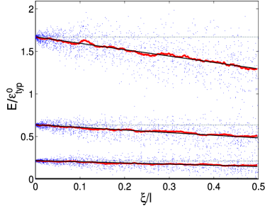
Figure 6: (Color online) Distribution of energies of fermionic subgap end states in a spinless $p$-wave superconductor with $N=7$ channels (dots), as a function of $\xi/l$. For small amounts of disorder the term $H^{(2)}$ dominates, pushing the subgap energies up or down with equal probability. At stronger disorder the term in $H^{(3{\rm b})}\propto\xi/l$ eventually dominates and pulls all energy levels towards zero. The red lines indicate the mean calculated from the local distribution of eigenvalues. The black lines, which are a linear fit to the mean values in red, share an approximate common intercept at the horizontal axis at $\xi/l=c^{-1}=2.2$. Dotted grey lines indicate the unperturbed energies. Energies are measured in units of $\varepsilon_{\text{typ}}^{0}=\Delta W^{2}/\xi^{2}$. The lattice parameters used in the numerical calculation correspond to $k_{F}W\approx 23$ and $k_{F}\xi\approx 320$.

V Smooth potential at wire’s end

In this section we consider a wire which is terminated by a smooth potential $V(x)$, as shown schematically in the inset of Fig. 7. In order to address this scenario we solve the Bogoliubov-de Gennes Hamiltonian in the WKB approximation. Without the transverse pairing term $H_{y}$ there are $N$ Majorana states $\psi^{(j)}$ with wavefunction

$$\psi^{(j)}({\boldsymbol{r}}) = \sqrt{\frac{2}{W}}\left(\begin{array}[]{c}e^{i\pi/4}\\ e^{-i\pi/4}\end{array}\right)\chi_{j}(x)\sin\left(\frac{n\pi y}{W}\right),$$ (36)

where the functions $\chi_{j}(x)$ take the form

$$\chi_{j}(x) = \left\{\begin{array}[]{ccc}\displaystyle\frac{e^{-x/\xi+\int_{x_{j}}^{x}dx^{\prime}\kappa_{j}(x^{\prime})}}{2\sqrt{\Omega_{j}\kappa_{j}(x)}}&\mbox{if $x<x_{j}$},\\ \displaystyle\frac{e^{-x/\xi}\cos[\Phi_{j}(x)]}{\sqrt{\Omega_{j}k_{j}(x)}}&\mbox{if $x>x_{j}$},\end{array}\right.$$ (39)

where $\Phi_{j}=\pi/4-\int_{x_{j}}^{x}dx^{\prime}k_{j}(x^{\prime})$,

$$k_{j}(x) = \sqrt{2m\left(\mu-V(x)-\frac{\pi^{2}n^{2}}{2mW^{2}}\right)-\frac{1}{\xi^{2}}},$$

$$\kappa_{j}(x) = \sqrt{\frac{1}{\xi^{2}}-2m\left(\mu-V(x)-\frac{\pi^{2}n^{2}}{2mW^{2}}\right)},$$

$\Omega_{j}$ is the normalization constant, and $x_{j}$ is the transverse-mode-dependent classical turning point, defined as the solution of $k_{j}(x_{j})=0$. Inclusion of the transverse pairing Hamiltonian $H_{y}$ lifts the degeneracy of the $N$ zero energy Majorana end states, where the energy splitting is given by the eigenvalues of the antisymmetric matrix with elements $H^{(1)}_{jl}=0$ if $j-l$ even and

$$H^{\rm(1)}_{jl} = \frac{16\Delta^{\prime}}{W}\frac{lj}{j^{2}-l^{2}}(X_{jl}^{(1)}+X_{jl}^{(2)}+X_{jl}^{(3)})$$ (40)

if $j-l$ odd, with, for $j<l$,

$$X_{jl}^{(1)} = \int_{-\infty}^{x_{j}}dx\frac{e^{-2x/\xi-\int_{x_{j}}^{x}dx^{\prime}\kappa_{j}(x^{\prime})-\int_{x_{l}}^{x}dx^{\prime}\kappa_{l}(x^{\prime})}}{4\sqrt{\Omega_{j}\Omega_{l}\kappa_{j}\kappa_{l}}},$$

$$X_{jl}^{(2)} = \int_{x_{j}}^{x_{l}}dx\frac{e^{-2x/\xi-\int_{x_{l}}^{x}\kappa_{l}}\cos[\Phi_{j}(x)]}{2\sqrt{\Omega_{j}\Omega_{l}k_{j}\kappa_{l}}},$$

$$X_{jl}^{(3)} = \int_{x_{l}}^{\infty}dx\frac{e^{-2x/\xi}\cos[\Phi_{j}(x)]\cos[\Phi_{l}(x)]}{\sqrt{\Omega_{j}\Omega_{l}k_{j}k_{l}}}.$$ (41)

Figure 7 shows numerical calculations for a lattice version of the spinless $p+ip$ model, with a potential $V(x)=ae^{-x^{2}/2\sigma^{2}}$, turning the hard-wall ending at $x=0$ effectively into a smooth end. The parameter $\sigma$ tunes the length scale over which the potential is turned on. The case $\sigma\to 0$ corresponds to a hard-wall boundary. The prefactor $a$ has the dimension of energy and determines the height of the potential. For the calculations shown in the figure, we chose $a=5\mu$. The results of the figure show a clear exponential dependence on $\sigma$ for states on the wire end terminated by the smooth function $V$, allowing for energies of the subgap states that are significantly below the (already small) estimates for a rectangular geometry with hard-wall boundary conditions.

The origin of the anomalously small energy splittings shown in Fig. 7 is the smoothness of all terms in the Hamiltonian $H$. If the $p+ip$ wire is coupled to a normal-metal stub, as in Sec. III, and the superconducting order parameter $\Delta$ jumps at the interface $x=0$, no reduction of the end-state energies is found, even if the normal-metal stub is terminated by a smooth potential. (This scenario is well described by the calculation of Sec. III.) On the other hand, one finds a suppression very similar to that shown in Fig. 7 if the superconducting order parameter goes to zero smoothly at the interface. We refere to Ref. Kells2012b, for a discussion of the effect of a smooth confinement in the semiconductor model.

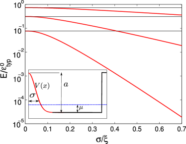
Figure 7: (Color online) Energies of fermionic subgap end states, in a $6$-channel $p+ip$ wire as function of the adiabaticity parameter $\sigma$ (red). The flat black lines indicate the energies for hard-wall boundary conditions ($\sigma=0$). Energies are measured in units of $\varepsilon_{\text{typ}}^{0}=\Delta W^{2}/\xi^{2}$. The lattice parameters used in the numerical calculation correspond to $k_{F}W\sim 19$ and $k_{F}\xi\sim 90$, $a=5\mu$. The inset shows the potential profile used in the calculations.

VI Conclusion

In this article, we have investigated fermionic subgap states localized near the end of a spinless $p$-wave superconducting wires for two terminations of the wire — a normal-metal stub and a smooth confining potential — and in the presence of weak disorder. The three scenarios give qualitatively different estimates for the energies of the subgap states. However, they share the common feature that a wire with $N$ transverse channels with a width $W$ that is much smaller than the superconducting coherence length $\xi$ has $\mbox{int}\,(N/2)$ fermionic end states, all with energy much below the bulk excitation gap $\Delta$. These states appear for the topological phase (which has a Majorana fermion at the wire’s end), as well as for the non-topological phase (which does not).

The appearance of low-energy fermionic end states poses an obstacle to the identification of Majorana fermions through a measurement of the tunneling density of states at the wire’s end, unless the energy resolution of the experiment is good enough to resolve the splitting between the fermionic end states. The corresponding energy scale $\varepsilon_{\rm min}$ scales proportional to $\Delta/k_{\rm F}\xi\sim\Delta^{2}/\mu$ in the most favorable scenario we considered (wire’s end coupled to a small normal metal stub), which is the same dependence as the subgap states in a vortex core.Caroli1964 The important difference with the subgap states in a vortex core is, however, that the number of fermionic end states is limited, so that there exists a maximum energy $\varepsilon_{\rm max}$, whereas no such maximum energy exists in a vortex. Other terminations, such as a rectangular end with or without disorder, or a smooth confinement potential, give significantly smaller values for $\varepsilon_{\rm min}$, and, hence, lead to stricter requirements for the energy resolution required to separate an eventual Majorana state from fermionic end states.

The recent experiments that reported the possible observation of a Majorana fermion involved semiconductor nanowires with proximity-induced superconductivity.Mourik2012 ; Das2012 Effectively, the induced superconductivity in these wires is of spinless $p$-wave type. However, it should be emphasized that this does not imply that the effective description of such a semiconductor wire with $N$ transverse channels is a $p+ip$ model with the same number of transverse channels. Instead, only those channels in the semiconductor that are effectively spinless (i.e., spin polarized or helical, depending on the relative strength of the applied magnetic field and the spin-orbit coupling) appear in the effective description in terms of a $p+ip$ model. (This latter distinction was overlooked in Ref. Tewari2012, .) Typically, this number is smaller than the number of transverse channels in the semiconductor. In particular, the nanowires of the experiments of Refs. Mourik2012, ; Das2012, are believed to be thin enough that they map to a single-channel $p+ip$ model. Hence, we do not expect that the mechanism for the generation of fermionic end states we consider applies to those experiments. However, it will apply to nanowires with a larger diameter, which we thus expect to exhibit a clustering of low-energy fermionic states in the topologically trivial as well as the topologically nontrivial phases. In this context, it is important to note that the condition that $W\ll\xi$ does not a priori prevent the applicability of our analysis to thicker wires, because the effective pairing potential $\Delta$ may decrease with $W$ for proximity-induced superconductivity in the limit of thick wires (see Ref. Duckheim2011, for an example in which $\Delta\propto W^{-1}$).

We gratefully acknowledge discussions with Felix von Oppen and Inanc Adagedeli. This work is supported by the Alexander von Humboldt Foundation in the framework of the Alexander von Humboldt Professorship, endowed by the Federal Ministry of Education and Research.

Appendix A Relationship between the $p+ip$ and proximity coupled semi-conductor models

A practical realization of a the $p+ip$ model can be found in semiconducting nanowires with strong spin-orbit coupling, laterally coupled to a standard $s$-wave superconductor and subject to a Zeeman field. In the following we discuss the precise relationship between the models. A related discussion can also be found in Ref. Alicea2010, .

In two dimensions, and without coupling to the superconductor, the Hamiltonian for this system reads

$$H_{\rm N} = \frac{p^{2}}{2m}-\mu+B\sigma_{x}+\alpha\sigma_{y}p_{x}-\alpha^{\prime}\sigma_{x}p_{y},$$ (42)

where $\alpha$ and $\alpha^{\prime}$ set the strength of the spin-orbit coupling and $B>0$ is the Zeeman energy of the applied magnetic field. In the limit of a narrow wire (width $W$ much smaller than the coherence length $\xi$ of the induced superconductivity), subgap states as well as the above-gap quasiparticle states have a vanishing expectation value of the transverse momentum $k_{y}$, which allows us to treat the transverse spin obit term as a perturbation, initially setting $\alpha^{\prime}=0$. Without the term proportional to $\alpha^{\prime}$ different transverse channels do not couple to each other and the eigenfunctions of the Hamiltonian $H_{\rm N}$ are of the form

$$\psi_{n,k}^{\pm}({\boldsymbol{r}})\propto\left(\begin{array}[]{c}e^{-i\theta_{k}}\\ \pm 1\end{array}\right)\frac{1}{\sqrt{W}}e^{ikx}\sin\frac{\pi ny}{W},$$ (43)

where the angle $\theta_{k}$ is defined as

$$\sin\theta_{k}=\frac{\alpha k}{\sqrt{B^{2}+\alpha^{2}k^{2}}},\ \ \cos\theta_{k}=\frac{B}{\sqrt{B^{2}+\alpha^{2}k^{2}}},$$ (44)

and the corresponding energies are

$$\varepsilon_{k,n}^{\pm}=\frac{\hbar^{2}k^{2}}{2m}+\frac{\hbar^{2}\pi^{2}n^{2}}{2mW^{2}}-\mu\pm\sqrt{B^{2}+\alpha^{2}k^{2}}.$$ (45)

Upon laterally coupling the semiconductor wire to an $s$-wave superconductor, the excitations are described by the Bogoliubov-de Gennes Hamiltonian

$$H_{\rm BdG} = \left(\begin{array}[]{cc}H_{\rm N}&\Delta\sigma_{y}\\ \Delta\sigma_{y}&-H_{\rm N}^{*}\end{array}\right)$$ (49)

$$= \left(\frac{p^{2}}{2m}-\mu+B\sigma_{x}+\alpha\sigma_{y}p_{x}\right)\tau_{z}$$

$$\mbox{}-\alpha^{\prime}\sigma_{x}p_{y}+\Delta\sigma_{y}\tau_{x},$$

where $\tau_{x}$, $\tau_{y}$, and $\tau_{z}$ are Pauli matrices in electron-hole space. Without the transverse spin-orbit coupling $\alpha^{\prime}$, the Bogoliubov-de Gennes Hamiltonian has a chiral symmetry, $\tau_{y}H\tau_{y}=-H$. In the basis of the normal-state eigenfunctions $\psi_{n,k}^{\pm}$, the Bogoliubov-de Gennes Hamiltonian (49) takes the form

$$H_{\rm BdG} = \left(\frac{\hbar^{2}k^{2}}{2m}+\frac{\hbar^{2}\pi^{2}n^{2}}{2mW^{2}}-\mu\right)\tau_{z}+\sigma_{z}\tau_{z}\sqrt{B^{2}+\alpha^{2}k^{2}}$$ (50)

$$\mbox{}+\Delta\sigma_{y}\tau_{x}\cos\theta_{k}+\Delta\sigma_{z}\tau_{x}\sin\theta_{k}$$

$$\mbox{}-\alpha^{\prime}p_{y}(\sigma_{z}\cos\theta_{k}+\sigma_{y}\sin\theta_{k}).$$

In the limit, when both $\Delta$ and the spin orbit energy are smaller than the Zeeman splitting, the $s$-wave pairing term proportional to $\sigma_{y}$ is ineffective, and each transverse channel separately maps to two spinless $p$-wave superconductors, one for $\psi_{n,k}^{+}$ and one for $\psi_{n,k}^{-}$. Neglecting $|\alpha k|$ in comparison to $B$, the corresponding pairing term $\Delta\sin\theta_{k}\sigma_{z}\tau_{x}\approx-\Delta^{\prime}k\sigma_{z}\tau_{x}$, with

$$\Delta^{\prime}=-\frac{\alpha\Delta}{B}.$$ (51)

Without the term proportional to $\alpha^{\prime}$, the transverse channels in Eq. (50) can be treated independently (at least in the bulk of the wire, see below). If $\mu<B$, only the “$-$” channels (eigenspinors of $\sigma_{z}$ with eigenvalue $-1$) in Eq. (50) are topologically nontrivial and can possibly have end states.Read2000 Projecting the Bogoliubov-de Gennes Hamiltonian in the rotated basis (50) onto these channels, one finds an effective Hamiltonian of the form

$$H_{\rm BdG}^{\rm eff} = \left(\frac{\hbar k^{2}}{2m}+\frac{\hbar^{2}\pi^{2}n^{2}}{2mW^{2}}-\mu-B\right)\tau_{z}$$ (52)

$$\mbox{}+\Delta^{\prime}\hbar k\tau_{x}+\alpha^{\prime}p_{y}\,,$$

Without the transverse spin-orbit coupling $\alpha^{\prime}$, the effective Hamiltonian (52) has chiral symmetry and $N$ Majorana end states at each end of the wire. The chiral symmetry is broken by the transverse spin-orbit coupling $\alpha^{\prime}$. Because of the particle-hole symmetry of the Majorana modes, the matrix elements of this perturbation between the $N$ Majorana end-state of $H_{\rm BdG}^{\rm eff}$ with $\alpha^{\prime}=0$ are the same as the matrix elements of the $p$-wave superconducting pairing $H_{y}$ of Eq. (2), if we identify $\Delta^{\prime}=\alpha^{\prime}$ in the expression for $H_{y}$.

If the condition $\mu<B$ is not met, the relation between the semiconductor and $p+ip$ models is more complicated. For transverse channels for which $\hbar^{2}\pi^{2}n^{2}/2mW^{2}<\mu-B$ the wire ends represent a chiral-symmetry-preserving perturbation that gaps out eventual Majorana end states, so that such channels may be disregarded when considering low-energy end states. For transverse channels for which

$$\mu-B<\frac{\hbar^{2}\pi^{2}n^{2}}{2mW^{2}}<\mu+B$$ (53)

the Majorana end state in the “$-$ band” (eigenspinors of $\sigma_{z}$ at eigenvalue $-1$ in the rotated basis) is protected in the presence of the chiral symmetry, and only perturbations that lift the chiral symmetry can lead to a splitting of these end states. Projecting the Bogoliubov-de Gennes Hamiltonian in the rotated basis (50) onto these channels, one again an effective Hamiltonian of the form (52), but with the additional restriction that only those transverse channels that meet the condition (53) are considered. The number $N$ of transverse channels that meet this condition may be smaller than the original number of propagating channels in the semiconductor.

References

- (1) C. W. J. Beenakker, arXiv:1112.1950v2 (2012).
- (2) J. Alicea Rep. Prog. Phys. 75, 076501 (2012)
- (3) A. Kitaev, Ann. Phys. 303, 2 (2003).
- (4) M. H. Freedman, Proc. Natl. Acad. Sci. U.S.A 95, 98 (1998).
- (5) N. Read and D. Green, Phys. Rev. B 61, 10267 (2000).
- (6) D. Ivanov, Phys. Rev. Lett. 86, 268 (2001).
- (7) A. Kitaev, Ann. Phys. 321, 2 (2006).
- (8) C. Nayak, S. H. Simon, A. Stern, M. Freedman, and S. Das Sarma, Rev. Mod. Phys. 80, 1083 (2008).
- (9) F. Wilczek, Nature Phys. 5, 614 (2009).
- (10) A. Y. Kitaev, Phys. Usp. 44, 131 (2001).
- (11) L. Fu and C. L. Kane, Phys. Rev. Lett. 100, 096407 (2008).
- (12) A. Cook and M. Franz, Phys. Rev. B 84, 201105(R) (2011).
- (13) J. D. Sau, R. M. Lutchyn, S. Tewari and S. Das Sarma, Phys. Rev. Lett. 104, 040502 (2010).
- (14) J. Alicea, Phys. Rev. B 81, 125318 (2010).
- (15) Y. Oreg, G. Refael, and F. von Oppen, Phys. Rev. Lett. 105, 177002 (2010).
- (16) R. M. Lutchyn, J. D. Sau, and S. Das Sarma, Phys. Rev. Lett. 105, 077001 (2010).
- (17) M. Duckheim and P. W. Brouwer, Phys. Rev. B 83, 054513 (2011).
- (18) S. B. Chung, H.-J. Zhang, X.-L. Qi, and S.-C. Zhang, Phys. Rev. B 84, 060510 (2011).
- (19) T.-P. Choy, J. M. Edge, A. R. Akhmerov, and C. W. J. Beenakker, Phys. Rev. B 84, 195442 (2011).
- (20) I. Martin and A. F. Morpurgo, Phys. Rev. B 85, 144505 (2012).
- (21) M. Kjaegaard, K. Wölms and K. Flensberg, Phys. Rev. B 85, 020503 (2012).
- (22) V. Mourik, K. Zuo, S. M. Frolov, S. R. Plissard, E. P. A. M. Bakkers, and L. P. Kouwenhoven, Science 336, 1003 (2012).
- (23) A. Das, Y. Ronen, Y. Most, Y. Oreg, M. Heiblum and H. Shtrikman, arXiv:1205.7073 (2012).
- (24) M. T. Deng, C. L. Yu, G. Y. Huang, M. Larsson, P. Caroff and H. Q. Xu, arXiv:1204.4130v1 (2012).
- (25) L. P. Rokhinson, X. Liu and J. K. Furdyna, arXiv:1204.4212v1 (2012).
- (26) J. R. Williams, A. J. Bestwick, P. Gallagher, S. S. Hong, Y. Cui, A. S. Bleich, J. G. Analytis, I. R. Fisher and D. Goldhaber-Gordon, arXiv:1202.2323v2 (2012).
- (27) G. Kells, D. Meidan and P. W Brouwer, Phys. Rev. B 85, 060507(R) (2012).
- (28) A. C. Potter and P. A. Lee, Phys. Rev. B 85 094516 (2012).
- (29) M. Gibertini, F. Taddei, M. Polini, R. Fazio, Phys. Rev. B 85, 144525 (2012).
- (30) S. Tewari. T. D. Stanescu, J. D. Sau and S. Das Sarma, Phys. Rev. B 86, 024504 (2012).
- (31) M. Wimmer, A. R. Akhmerov, M. V. Medvedyeva, J. Tworzydlo, and C. W. J. Beenakker, Phys. Rev. Lett. 105, 046803 (2010).
- (32) A. C. Potter and P. A. Lee, Phys. Rev. Lett. 105, 227003 (2010).
- (33) R. M. Lutchyn, T. D. Stanescu, and S. Das Sarma, Phys. Rev. Lett. 106, 127001 (2011).
- (34) A. C. Potter and P. A. Lee, Phys. Rev. B 83 184520 (2011); Phys. Rev. B 84 059906(E) (2011).
- (35) T. Stanescu, R. M. Lutchyn, and S. Das Sarma, Phys. Rev. B 84, 144522 (2011).
- (36) B. Zhou and S.-Q. Shen, Phys. Rev. B 84, 054532 (2011).
- (37) J. S. Lim, L. Serra, R. Lopez, and R. Aguado arXiv:1202.5057 (2012).
- (38) C. Caroli, P. G. De Gennes, and J. Matricon, Phys. Letters 9, 307 (1964).
- (39) O. Motrunich, K. Damle, and D. A. Huse, Phys. Rev. B 63, 224204 (2001).
- (40) P. W. Brouwer, M. Duckheim, A. Romito and F. von Oppen, Phys. Rev. Lett. 107, 196804 (2011).
- (41) S. Tewari, J. D. Sau arXiv:1111.6592 (2011).
- (42) E. P. Wigner, Phys. Rev. 98, 145 (1955).
- (43) F. T. Smith , Phys. Rev. 118 349 (1960).
- (44) C. W. J. Beenakker, Rev. Mod. Phys. 3, 731 (1997).
- (45) P. W. Brouwer, K. M. Frahm, and C. W. J. Beenakker, Phys. Rev. Lett. 78 4737 (1997).
- (46) J. N. H. J. Cremers and P. W. Brouwer, Phys. Rev. B 65, 115333 (2002).
- (47) J. A. Melsen. P. W. Brouwer, K. M. Frahm and C. W. J. Beenakker Europhys. Lett. 35, 7 (1996).
- (48) T. Kato, Prog. Theor. Phys. , 4 514, (1949).
- (49) C. Bloch, Nuclear Physics, 6 329 (1958).
- (50) See Chapter 16, Secs. 15–17 of A. Messiah, Quantum Mechanics, North Holland (1961).
- (51) S. P. Jordan and E. Farhi, Phys. Rev. A 77, 062329 (2008).
- (52) G. Kells, D. Meidan, and P. W. Brouwer preprint.