Geometry of deadbeat synchronization

Abstract

The deadbeat synchronization of identical discrete-time nonlinear systems is studied from a geometric point of view. An array of deadbeat observers coupled via a deadbeat interconnection is shown to achieve synchronization in finite number of steps provided that a compatibility condition is satisfied between the observer and the interconnection. As an illustration to the theory, an example is provided where an array of third order observers achieves deadbeat synchronization.

1 Introduction

Two or more dynamical systems are said to synchronize when their solutions converge to a common trajectory. The generality of this definition allows many seemingly different cases to make examples of synchronization [1]. One such example is the following pair of discrete-time linear systems

$$x_{1}^{+}&=Ax_{1}\\ x_{2}^{+}=Ax_{2}+L(y_{1}-y_{2})$$ (1)

where $y_{i}=Cx_{i}$ and all the eigenvalues of the matrix $A-LC$ are on the open unit disc. The second system (1b) is the classic linear observer [2] and its construction readily yields $\|x_{1}(k)-x_{2}(k)\|\to 0$ as $k\to\infty$ regardless of the initial conditions. Another linear example to synchronization is the following array of systems with rather simple dynamics

$$y_{i}^{+}=\sum_{j=1}^{q}\gamma_{ij}y_{j}\,,\qquad i=1,\,2,\,\ldots,\,q$$ (2)

where $[\gamma_{ij}]\in{\mathbb{R}}^{q\times q}$ is a (connected) coupling matrix. That is, $[\gamma_{ij}]$ satisfies: (i) the entries of each row sum up to unity, which implies that $\lambda=1$ is an eigenvalue with the eigenvector $[1\ \ 1\ \ldots\ 1]^{T}$, and (ii) all the remaining eigenvalues are on the open unit disc. In this case the solutions $y_{i}(k)$ converge to a fixed point in space and the systems are said to reach consensus [3, 4].

At first sight the arrays (1) and (2) may not seem to be relevant, but they are in fact the two limiting cases of the following general structure

$$x_{i}^{+} = Ax_{i}+L\left(\sum_{j=1}^{q}\gamma_{ij}y_{j}-y_{i}\right)\,,\qquad i=1,\,2,\,\ldots,\,q$$ (3)

$$y_{i} = Cx_{i}\,.$$

Note that (3) boils down to (1) for

$$[\gamma_{ij}]=\left[\begin{array}[]{rr}1&0\\ 1&0\end{array}\right]$$

and to (2) for $A=C=L=I$. An effective way to study the synchronization behavior of an array is through understanding the smaller pieces that it is made of [5, 6, 7]. So if the array (3) is what we are trying to understand then it is worthwhile to focus on its two limiting cases: the array (1) and the array (2). In this line of thinking, the very first question that one is tempted to ask is the following. Given that the system (1b) is an observer for the system (1a) and that the array (2) reaches consensus, does the array (3) synchronize? However, a counterexample is easy to construct and this naive guess has to be abandoned.

Having dispensed with the first question, we point our attention, among a number of possibilities, to the following. Given that the system (1b) is a deadbeat observer [8, 9, 10] for the system (1a) and that the array (2) reaches consensus in finite number of steps [11, 12], does the array (3) synchronize? This guess turns out to be more fruitful than the first one. In fact not only synchronization is achieved in this case, but it is achieved in deadbeat fashion, that is, in finite number of steps. Motivated by this simple observation on linear systems, we aim in this paper to establish sufficient conditions that guarantee deadbeat synchronization in an array of coupled identical discrete-time nonlinear systems. What we particularly study here is the synchronization behavior of an array of deadbeat observers that are coupled through a fixed interconnection scheme, which itself, if considered separately as the righthand side of an array, enjoys deadbeat synchronization. We show that deadbeat synchronization is achieved under a compatibility condition between the observer and the interconnection.

The literature accommodates few results on deadbeat synchronization. Motivated by possible applications in secure communications, one of the earliest results on the subject is presented in [13], where conditions for the synchronization of two systems of type Lur’e, coupled via a scalar output signal are given. Later, certain improvements to this work are reported, for instance, in [14, 15, 16], where synchronization still requires that the number of systems is two and the output is scalar. To the best of our knowledge, the problem of deadbeat synchronization has not yet been considered in a general setting where the number of (identical, nonlinear) individual systems are arbitrary and the output signals, through which the systems are coupled, are not necessarily scalar. The contribution of this paper is hence intended to be in understanding better the mechanism behind synchronization in discrete time from the deadbeat point of view.

The remainder of the paper is organized as follows. The next section contains some preliminary material. In Section 3 is the construction of the deadbeat observer, which is of geometric nature [17, 18] and makes a special case of what is presented in [10]. The reader will find an illustrative example following this construction. As mentioned earlier, the observer together with the system being observed make a particular case of synchronization where there are only two systems. To reach a natural generalization of this scenario we take two mental steps. First, we remove the distinction between the two systems by allowing each to observe the other. In other words, we dispense with the drive system (leader)-response system (follower) hierarchy. Second, having removed the distinction between the observer and the observee, we allow the number of systems involved to be arbitrary. At that point a method is required to couple this array of observers. Therefore we introduce in Section 4 what we call deadbeat interconnection, which basically is a nonlinear generalization of the time-invariant map (coupling matrix) that appears in linear deadbeat consensus. Then in Section 5 we bring together the observer construction of Section 3 and the interconnection scheme of Section 4 to define the array of coupled observers. There we establish the deadbeat synchronization of this array under a compatibility condition that concerns both the observer and the interconnection. In Section 6 we provide a nonlinear example where an array of third order deadbeat observers are shown to achieve deadbeat synchronization. Certain issues are discussed in Section 7.

2 Preliminaries

The set of nonnegative integers is denoted by ${\mathbb{N}}$, the set of rational numbers by ${\mathbb{Q}}$. A vector of all ones is denoted by ${\mathbf{1}}$. The $m\times m$ identity matrix is denoted by $I_{m}$, or sometimes simply by $I$ when what $m$ should be is either obvious or immaterial. The symbol $\otimes$ denotes Kronecker product. The null space of a matrix $M\in{\mathbb{R}}^{m\times n}$ is denoted by $\mathcal{N}(M)$ and $M^{\perp}$ denotes some real matrix, whose columns form a basis for $\mathcal{N}(M)$. For square $M$ we let $M^{0}=I$. Given a map $h:\mathcal{X}\to\mathcal{Y}$, $h^{-1}$ denotes the inverse map in the general sense that, for $y\in\mathcal{Y}$, $h^{-1}(y)$ is the set of all $x\in\mathcal{X}$ satisfying $h(x)=y$. That is, we will not need $h$ be bijective when talking about its inverse. For $f:\mathcal{X}\to\mathcal{X}$ we let $f^{0}(x)=x$, $f^{k+1}(x)=f(f^{k}(x))$, and $f^{-k}=(f^{-1})^{k}$ for $k\in{\mathbb{N}}$. Given vectors $x_{1},\,x_{2},\,\ldots,\,x_{q}\in{\mathbb{R}}^{n}$ we write $(x_{1},\,x_{2},\,\ldots,\,x_{q})$ to mean $[x_{1}^{T}\ x_{2}^{T}\ \ldots\ x_{q}^{T}]^{T}\in{\mathbb{R}}^{qn}$. We sometimes use “$*$” as a placeholder for “don’t care.”

3 Deadbeat observer

This section is dedicated to the description of the nonlinear deadbeat observer. Later, in Section 5, when we establish the conditions for deadbeat synchronization of an array of coupled observers, the construction presented here will be of key importance. Unlike linear systems, there is not a standard deadbeat observer construction for nonlinear systems. Even the definition of a deadbeat observer may not be unique. The definition and the construction that we present in this section are adopted from [10]. The section ends with an illustration of the construction.

3.1 Definition

Consider the following discrete-time system

$$x^{+}=f(x)\,,\quad y=h(x)$$ (5)

where $x\in\mathcal{X}\subset{\mathbb{R}}^{n}$ is the state, $x^{+}$ is the state at the next time instant, and $y\in h(\mathcal{X})=:\mathcal{Y}\subset{\mathbb{R}}^{m}$ is the output or the measurement. The solution of the system (5) at time $k\in{\mathbb{N}}$, starting at the initial condition $x(0)\in\mathcal{X}$ is denoted by $x(k)$. Now consider the following array

$$x^{+}&=f(x)\\ \hat{x}^{+}=g(\hat{x},\,h(x))\,.$$ (6)

The solution of the system (6b) at time $k\in{\mathbb{N}}$, starting at the initial condition $\hat{x}(0)\in\mathcal{X}$ is denoted by $\hat{x}(k)$. Note that $\hat{x}(k)$ depends also on $x(0)$. We now use (6) to define deadbeat observer.

Definition 1

Given $g:\mathcal{X}\times\mathcal{Y}\to\mathcal{X}$, the system

$$\hat{x}^{+}=g(\hat{x},\,y)$$

is said to be a deadbeat observer for the system (5) if there exists an integer $p\geq 1$ such that, for all initial conditions, the solutions of the array (6) satisfy $\hat{x}(k)=x(k)$ for all $k\geq p$. The integer $p$ then is called a deadbeat horizon.

3.2 Construction

To be used in the construction of the observer we define certain sets associated with the system (5). For $x\in\mathcal{X}$ we let

$$[x]_{0}:=h^{-1}(h(x))\,.$$

Note that when $h(x)=Cx$, where $C\in{\mathbb{R}}^{m\times n}$, we have $[x]_{0}=x+\mathcal{N}(C)$. We then let for $k\in{\mathbb{N}}$

$$[x]_{k+1}:=[x]_{k}^{+}\cap[x]_{0}$$

where

$$[x]_{k}^{+}:=f([f^{-1}(x)]_{k})\,.$$

We finally let

$$[x]_{-1}^{+}:=\mathcal{X}\,.$$

We make the following two assumptions to guarantee that the observer construction will work. We note that these conditions are only sufficient. For less restrictive assumptions see [10].

Assumption 1

The map $f:\mathcal{X}\to\mathcal{X}$ is bijective.

Assumption 2

There exists $p\geq 1$ such that $[\hat{x}]_{p-2}^{+}\cap h^{-1}(y)$ is singleton for all $\hat{x}\in\mathcal{X}$ and $y\in\mathcal{Y}$.

The following result tells us how to design a deadbeat observer under these assumptions.

Theorem 1

Suppose Assumptions 1-2 hold. Then the system

$$\hat{x}^{+}=f([\hat{x}]^{+}_{p-2}\cap h^{-1}(y))$$ (7)

is a deadbeat observer for the system (5) with deadbeat horizon $p$.

Theorem 1 will later become a corollary of our main result (Theorem 4). Hence we omit the proof. Let us now give an example to this construction (7).

3.3 Illustration

Consider the system (5) with

$$f(x)=\left[\begin{array}[]{c}1+\xi_{2}-a\xi_{1}^{2}\\ b\xi_{1}+\xi_{3}\\ -b\xi_{1}\end{array}\right]$$

where $x=(\xi_{1},\,\xi_{2},\,\xi_{3})\in{\mathbb{R}}^{3}$. This map appears in [19] where it is reported to exhibit chaotic behavior for certain values of real numbers $a$ and $b$. Let us now construct a deadbeat observer taking $h(x)=\xi_{3}$. Note first that $f$ is bijective (for $b$ nonzero) and its inverse is

$$f^{-1}(x)=\left[\begin{array}[]{c}-b^{-1}\xi_{3}\\ -1+ab^{-2}\xi_{3}^{2}+\xi_{1}\\ \xi_{2}+\xi_{3}\end{array}\right]$$ (12)

Since $h(x)=\xi_{3}$ we can write

$$[x]_{0}=\left\{\left[\begin{array}[]{c}s\\ t\\ \xi_{3}\end{array}\right]:s,\,t\in{\mathbb{R}}\right\}$$ (16)

Then by (12)

$$[x]_{0}^{+} = f([f^{-1}(x)]_{0})$$ (20)

$$= f\left(\left\{\left[\begin{array}[]{c}s\\ t\\ \xi_{2}+\xi_{3}\end{array}\right]:s,\,t\in{\mathbb{R}}\right\}\right)$$

$$= \left\{\left[\begin{array}[]{c}t\\ s+\xi_{2}+\xi_{3}\\ -s\end{array}\right]:s,\,t\in{\mathbb{R}}\right\}$$ (24)

The set $[x]_{1}$ is defined to equal $[x]_{0}^{+}\cap[x]_{0}$. The intersection of the sets (16) and (20) yields

$$[x]_{1}=\left\{\left[\begin{array}[]{c}u\\ \xi_{2}\\ \xi_{3}\end{array}\right]:u\in{\mathbb{R}}\right\}$$

Now we can construct $[x]_{1}^{+}$ as

$$[x]_{1}^{+} = f([f^{-1}(x)]_{1})$$

$$= f\left(\left\{\left[\begin{array}[]{c}u\\ -1+ab^{-2}\xi_{3}^{2}+\xi_{1}\\ \xi_{2}+\xi_{3}\end{array}\right]:u\in{\mathbb{R}}\right\}\right)$$

$$= \left\{\left[\begin{array}[]{c}\xi_{1}+ab^{-2}\xi_{3}^{2}-au^{2}\\ bu+\xi_{2}+\xi_{3}\\ -bu\end{array}\right]:u\in{\mathbb{R}}\right\}$$

Observe that

$$[\hat{x}]_{1}^{+}\cap h^{-1}(y) = \left\{\left[\begin{array}[]{c}\hat{\xi}_{1}+ab^{-2}\hat{\xi}_{3}^{2}-au^{2}\\ bu+\hat{\xi}_{2}+\hat{\xi}_{3}\\ -bu\end{array}\right]:u\in{\mathbb{R}}\right\}\cap\left\{\left[\begin{array}[]{c}s\\ t\\ y\end{array}\right]:s,\,t\in{\mathbb{R}}\right\}$$

$$= \left[\begin{array}[]{c}\hat{\xi}_{1}+ab^{-2}(\hat{\xi}_{3}^{2}-y^{2})\\ \hat{\xi}_{2}+\hat{\xi}_{3}-y\\ y\end{array}\right]$$

which means that Assumption 2 is satisfied with $p=3$. The dynamics of the deadbeat observer then read

$$\hat{x}^{+} = f([\hat{x}]_{1}^{+}\cap h^{-1}(y))$$

$$= \left[\!\!\begin{array}[]{c}1+\hat{\xi}_{2}+\hat{\xi}_{3}-y-a(\hat{\xi}_{1}+ab^{-2}(\hat{\xi}_{3}^{2}-y^{2}))^{2}\\ b\hat{\xi}_{1}+ab^{-1}(\hat{\xi}_{3}^{2}-y^{2})+y\\ -b\hat{\xi}_{1}-ab^{-1}(\hat{\xi}_{3}^{2}-y^{2})\end{array}\!\!\right]$$

For the parameter choice $a=1$ and $b=1/3$, Fig. 1 shows the simulation results for the initial conditions $x(0)=(1,\,-1,\,1)$ and $\hat{x}(0)=(0,\,2,\,1)$.

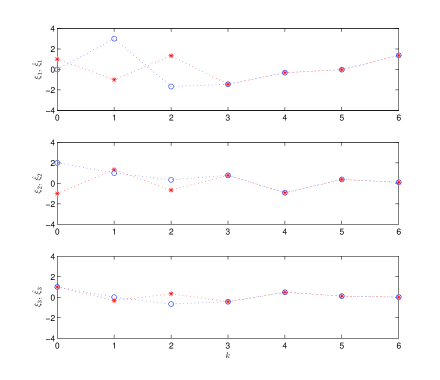
Figure 1: Evolution of states $x$ (marked $*$) and $\hat{x}$ (marked $\circ$).

The description of the deadbeat observer is now complete. As mentioned earlier, we are headed towards understanding the collective behavior of an arbitrary number of identical observers that are interacting. To be able to proceed, we therefore first need to be precise with what we mean by interacting. To this end, we introduce in the next section the so called deadbeat interconnection. This interconnection scheme will be evoked in Section 5 to characterize the coupling of the array whose synchronization we will study.

4 Deadbeat interconnection

Here we provide a generalization of the case where the linear array (2) reaches consensus in finite number of steps, which happens when the characteristic polynomial of the $q\times q$ coupling matrix $[\gamma_{ij}]$ is $d(s)=s^{q-1}(s-1)$. When referring to such $[\gamma_{ij}]$ we will use the term deadbeat coupling matrix. A primitive example for $q=4$ is given as

$$[\gamma_{ij}]=\left[\begin{array}[]{rrrr}0.4&-0.2&3.2&-2.4\\ 0.4&-0.2&0.2&0.6\\ 0.2&-0.6&0.6&0.8\\ 0.3&-0.4&0.9&0.2\end{array}\right]$$ (35)

which yields

$$[\gamma_{ij}]^{k}=\left[\begin{array}[]{rrrr}0.1&-0.8&1.3&0.4\\ 0.1&-0.8&1.3&0.4\\ 0.1&-0.8&1.3&0.4\\ 0.1&-0.8&1.3&0.4\end{array}\right]=\left[\begin{array}[]{r}1\\ 1\\ 1\\ 1\end{array}\right]\times[0.1\ \ -0.8\ \ 1.3\ \ 0.4]$$

for all $k\geq 3$. This means that the solutions of the array (2) should satisfy $y_{i}(k)=0.1y_{1}(0)-0.8y_{2}(0)+1.3y_{3}(0)+0.4y_{4}(0)$ for all $k\geq 3$. That is, convergence is exact. Now we give the generalization.

Definition 2

A map $\gamma=(\gamma_{1},\,\gamma_{2},\,\ldots,\,\gamma_{q})$ with $\gamma_{i}:\mathcal{Y}^{q}\to\mathcal{Y}$ is said to be a deadbeat interconnection if the following conditions simultaneously hold.

• There exists an integer $r\geq 1$ such that, for all initial conditions, the solutions of the array

  $$y_{i}^{+} = \gamma_{i}(y_{1},\,y_{2},\,\ldots,\,y_{q})\,,\qquad i=1,\,2,\,\ldots,\,q$$

  satisfy $y_{i}(k)=y_{j}(k)$ for all $k\geq r$ and all $i,\,j$. The integer $r$ then is called a deadbeat horizon.

• For all $y\in\mathcal{Y}$ we have $\gamma_{i}(y,\,y,\,\ldots,\,y)=\gamma_{j}(y,\,y,\,\ldots,\,y)$ for all $i,\,j$.

Some examples are in order. Let $G\in{\mathbb{R}}^{q\times q}$ be a deadbeat coupling matrix and $\mathcal{Y}={\mathbb{R}}^{m}$. Then the linear map

$${\mathbf{y}}\mapsto(G\otimes Q){\mathbf{y}}$$ (37)

with ${\mathbf{y}}=(y_{1},\,y_{2},\,\ldots,\,y_{q})$ is a deadbeat interconnection for any $Q\in{\mathbb{R}}^{m\times m}$. Note for $Q=I$ that the array (2) makes a special case of this construction. Not all linear deadbeat interconnections must have this structure (37) though. For instance, for $\mathcal{Y}={\mathbb{R}}^{2}$ and $q=2$, the map ${\mathbf{y}}\mapsto\Gamma{\mathbf{y}}$ with

$$\Gamma=\left[\begin{array}[]{rrrr}0&0&1&0\\ 0&1&0&0\\ 0&0&1&0\\ 1&1&-1&0\end{array}\right]$$ (42)

can be shown to be a deadbeat interconnection for which no $G,\,Q\in{\mathbb{R}}^{2\times 2}$ exist that yield $G\otimes Q=\Gamma$. Our last example is nonlinear. Let $[\gamma_{ij}]\in{\mathbb{R}}^{q\times q}$ be a deadbeat coupling matrix and $\mathcal{Y}={\mathbb{R}}$. Then the map $\gamma=(\gamma_{1},\,\gamma_{2},\,\ldots,\,\gamma_{q})$ with

$$\gamma_{i}({\mathbf{y}})=\left(\sum_{j=1}^{q}\gamma_{ij}y_{j}^{3}\right)^{1/3}$$ (43)

is a deadbeat interconnection.

Recall that in the standard observer setting, where there are only two systems in the array, i.e., the response system (the observer) and the drive system (the system being observed); the driving signal for the observer is the output of the system being observed. When one considers the general setting, where the array contains an arbitrary number of systems, the driving signal of each system (observer) is a function of the outputs of all the systems in the array. An array with $q$ many systems means there will be $q$ such functions. The deadbeat interconnection $(\gamma_{1},\,\gamma_{2},\,\ldots,\,\gamma_{q})$ we defined in this section is nothing but a particular collection of those coupling functions. Having defined deadbeat observer and deadbeat interconnection, now we proceed to study the array that we form by bringing the two together.

5 Deadbeat synchronization

This section is where we finally gather the conditions that yield deadbeat synchronization of an array of coupled identical observers. Let us begin with defining the phenomenon under investigation.

Definition 3

Given the maps $g:\mathcal{X}\times\mathcal{Y}\to\mathcal{X}$, $h:\mathcal{X}\to\mathcal{Y}$, and $(\gamma_{1},\,\gamma_{2},\,\ldots,\,\gamma_{q})=\gamma:\mathcal{Y}^{q}\to\mathcal{Y}^{q}$, the following array

$$x_{i}^{+} = g(x_{i},\,w_{i})\,,\qquad i=1,\,2,\,\ldots,\,q$$ (44)

$$w_{i} = \gamma_{i}(h(x_{1}),\,h(x_{2}),\,\ldots,\,h(x_{q}))$$

is said to achieve deadbeat synchronization if there exists an integer $\tau\geq 1$ such that, for all initial conditions, the solutions satisfy $x_{i}(k)=x_{j}(k)$ for all $k\geq\tau$ and all $i,\,j$. The integer $\tau$ then is called a deadbeat horizon.

This definition lets us write the formal statement of the problem to which we propose a solution in this paper: Under what conditions on the triple $(g,\,h,\,\gamma)$ does the array (44) achieve deadbeat synchronization? Now, instead of directly listing the assumptions and establishing the main result, we prefer first to present the linear case, which we mentioned in the introduction in a slightly less general form (3), that motivated all the analysis in this paper. The conditions on which this linear result is founded we take as a justification for some of the assumptions we will have made.

Theorem 2

Let $A\in{\mathbb{R}}^{n\times n}$, $C\in{\mathbb{R}}^{m\times n}$, and $L\in{\mathbb{R}}^{n\times m}$ be such that $A-LC$ is nilpotent. Let $[\gamma_{ij}]\in{\mathbb{R}}^{q\times q}$ be a deadbeat coupling matrix. Then the array

$$x_{i}^{+} = Ax_{i}+L\left(\sum_{j=1}^{q}\gamma_{ij}Qy_{j}-y_{i}\right)\,,\qquad i=1,\,2,\,\ldots,\,q$$ (45)

$$y_{i} = Cx_{i}$$

achieves deadbeat synchronization for all $Q\in{\mathbb{R}}^{m\times m}$. In particular, for all initial conditions, we have $x_{i}(k)=x_{j}(k)$ for all $k\geq rp$ and all $i,\,j$; where the integers $r\geq 1$ and $p\geq 1$ satisfy $[\gamma_{ij}]^{r}=[\gamma_{ij}]^{r+1}$ and $(A-LC)^{p}=0$.

Proof. First let ${\mathbf{x}}=(x_{1},\,x_{2},\,\ldots,\,x_{q})$ and $G:=[\gamma_{ij}]$. Then the array (45) can be written as

$${\mathbf{x}}^{+}=\left[I_{q}\otimes A+(I_{q}\otimes L)(G\otimes Q-I_{qm})(I_{q}\otimes C)\right]{\mathbf{x}}\,.$$

Since $G$ is a deadbeat coupling matrix we have $G^{r}={\mathbf{1}}\ell^{T}$ where $\ell\in{\mathbb{R}}^{q}$ is the left eigenvector of $G$ for the eigenvalue $\lambda=1$ satisfying $\ell^{T}{\mathbf{1}}=1$. That all the remaining eigenvalues are at the origin allows us to find a transformation matrix $V\in{\mathbb{R}}^{q\times q}$ satisfying

$$V=[{\mathbf{1}}\ *]\quad\mbox{and}\quad V^{-1}=[\ell\ *]^{T}$$

as well as

$$V^{-1}GV=\left[\begin{array}[]{cc}1&0\\ 0&J\end{array}\right]$$

for some $J\in{\mathbb{R}}^{(q-1)\times(q-1)}$ that is strictly upper triangular. Without loss of generality we assume that $J$ is in Jordan form. That is, $J={\rm diag}(J_{1},\,J_{2},\,\ldots,\,J_{\sigma})$ where each (Jordan) block $J_{\alpha}$, $\alpha\in\{1,\,2,\,\ldots,\,\sigma\}$, is strictly upper triangular. Then the size of the largest Jordan block is no greater than $r\times r$. Employing the coordinate change ${\mathbf{z}}:=(V^{-1}\otimes I_{n}){\mathbf{x}}$ we can write

$${\mathbf{z}}^{+} = (V^{-1}\otimes I_{n})\left[I_{q}\otimes A+(I_{q}\otimes L)(G\otimes Q-I_{qm})(I_{q}\otimes C)\right](V\otimes I_{n}){\mathbf{z}}$$ (49)

$$= \left[I_{q}\otimes A+(I_{q}\otimes L)(V^{-1}\otimes I_{m})(G\otimes Q-I_{qm})(V\otimes I_{m})(I_{q}\otimes C)\right]{\mathbf{z}}$$

$$= \left[I_{q}\otimes A+(I_{q}\otimes L)(V^{-1}GV\otimes Q-I_{qm})(I_{q}\otimes C)\right]{\mathbf{z}}$$

$$= \left[\begin{array}[]{cc}A+L(Q-I_{m})C&0\\ 0&N\end{array}\right]{\mathbf{z}}$$

where

$$N=I_{q-1}\otimes A+(I_{q-1}\otimes L)(J\otimes Q-I_{(q-1)m})(I_{q-1}\otimes C)\,.$$

Since $J$ is block diagonal with blocks strictly upper triangular, $N$ is also block diagonal $N={\rm diag}(N_{1},\,N_{2},\,\ldots,\,N_{\sigma})$ with the structure

$$N_{\alpha}=\left[\begin{array}[]{ccccc}A-LC&*&*&\cdots&*\\ 0&A-LC&*&\cdots&*\\ 0&0&A-LC&\cdots&*\\ \vdots&\vdots&\vdots&\ddots&\vdots\\ 0&0&0&\cdots&A-LC\end{array}\right]$$

for all $\alpha\in\{1,\,2,\,\ldots,\,\sigma\}$. Note that the size of the largest of the blocks $N_{\alpha}$ is no greater than $rn\times rn$. And this largest block must vanish in $rp$ steps because $(A-LC)^{p}=0$. By the time the largest block has vanished the other blocks must have also vanished. We deduce therefore

$$N^{rp}=0\,.$$ (51)

Equations (49) and (51) yield

$${\mathbf{x}}(k)=[{\mathbf{1}}\ell^{T}\otimes(A+L(Q-I_{m})C)^{k}]{\mathbf{x}}(0)$$

for all $k\geq rp$. In other words, all the solutions $x_{i}(\cdot)$ converge (in deadbeat fashion) to the trajectory

$${\bar{x}}(k)=(A+LQC-LC)^{k}\bar{x}(0)$$

where $\bar{x}(0)=(\ell^{T}\otimes I_{n}){\mathbf{x}}(0)$.   $\blacksquare$

Remark 1

The proof of Theorem 2 reveals that the array (45) would still achieve synchronization (not in finite number of steps, but asymptotically) with deadbeat interconnection even if the matrix $A-LC$ was not nilpotent, but only convergent, i.e., $(A-LC)^{k}\to 0$ as $k\to\infty$.

Remark 2

Another point made apparent by the proof of Theorem 2 is the following. Instead of the fixed interconnection ${\mathbf{y}}\mapsto(G\otimes Q){\mathbf{y}}$ if we employed a time-varying one with the structure ${\mathbf{y}}\mapsto(G\otimes Q_{k}){\mathbf{y}}$, the array (45) would still achieve deadbeat synchronization (with the same deadbeat horizon) regardless of how matrix $Q_{k}$ changes in time.

Let us go through the conditions required for Theorem 2 in order to generate their nonlinear counterparts. One condition is that the matrix $A-LC$ is nilpotent. This is equivalent to that the system (1b) is a deadbeat observer for the system (1a), which suggests for the nonlinear case that each individual system of the array is a deadbeat observer. Recall that, under Assumptions 1-2, we know how to construct a deadbeat observer, see Theorem 1. Another condition in Theorem 2 is that $[\gamma_{ij}]$ is a deadbeat coupling matrix. This translates into that the map ${\mathbf{y}}\mapsto([\gamma_{ij}]\otimes Q){\mathbf{y}}$ is a deadbeat interconnection. Hence the following assumption, which we will later need for the main theorem.

Assumption 3

The map $\gamma=(\gamma_{1},\,\gamma_{2},\,\ldots,\,\gamma_{q})$ is a deadbeat interconnection with deadbeat horizon $r$.

Consider now, in the light of Theorem 1 and under Assumptions 1-3, the following array

$$x_{i}^{+} = f([x_{i}]_{p-2}^{+}\cap h^{-1}(w_{i}))\,,\qquad i=1,\,2,\,\ldots,\,q$$ (52)

$$w_{i} = \gamma_{i}(h(x_{1}),\,h(x_{2}),\,\ldots,\,h(x_{q}))\,.$$

Does the array (52) achieve deadbeat synchronization? The answer to this question is negative and that is why we will eventually need to make a fourth assumption. A counterexample, which is indeed linear, is as follows.

We take $\mathcal{X}={\mathbb{R}}^{4}$ and $\mathcal{Y}={\mathbb{R}}^{2}$. Let $f(x)=Ax$ and $h(x)=Cx$ with

$$A=\left[\begin{array}[]{rrrr}0&-1&1&0\\ -1&0&0&-1\\ 1&0&0&0\\ -1&-1&-1&1\end{array}\right]\quad\mbox{and}\quad C=\left[\begin{array}[]{rrrr}0&-1&1&-1\\ -1&1&0&1\end{array}\right]$$

Assumption 1 is satisfied since $A$ is nonsingular. Assumption 2 is also satisfied (with $p=2$) because

$$[x]_{0}^{+}\cap h^{-1}(y)=x+H(y-Cx)$$

where $H$ can be computed as

$$H=AC^{\perp}(CAC^{\perp})^{-1}=\left[\begin{array}[]{rr}-1&-5/4\\ 1&6/4\\ 0&-1/4\\ -2&-7/4\end{array}\right]$$

Note that $(A-AHC)^{2}=0$. As for the deadbeat interconnection, we take $\gamma({\mathbf{y}})=\Gamma{\mathbf{y}}$ where $\Gamma\in{\mathbb{R}}^{4\times 4}$ is as in (42), which is known to satisfy Assumption 3 without admitting matrices $G,\,Q\in{\mathbb{R}}^{2\times 2}$ to realize $G\otimes Q=\Gamma$. (We especially want to emphasize here that the special structure (37) of the interconnection assumed in Theorem 2 is not merely for demonstrational convenience. The structure (37) does indeed play a role in achieving synchronization.) Hence the triple $(f,\,h,\,\gamma)=(A,\,C,\,\Gamma)$ satisfies Assumptions 1-3. Under our parameter choice the array (52) enjoys the following form

$$\left[\begin{array}[]{c}x_{1}\\ x_{2}\end{array}\right]^{+}=\underbrace{(I_{2}\otimes A)(I_{8}+(I_{2}\otimes H)(\Gamma-I_{4})(I_{2}\otimes C))}_{\displaystyle\Phi}\left[\begin{array}[]{c}x_{1}\\ x_{2}\end{array}\right]$$

which does not achieve deadbeat synchronization. Because if it did then it would necessarily require that the matrix $\Phi\in{\mathbb{R}}^{8\times 8}$ has at least $(q-1)n=4$ of its eigenvalues at the origin. However, the characteristic polynomial of $\Phi$ turns out to be $d(s)=s^{8}-3.5s^{7}-1.5s^{6}+11.5s^{5}-2.5s^{4}-8s^{3}-2s^{2}$.

This example justifies that Assumptions 1-3 are not sufficient and additional conditions are needed for the deadbeat synchronization of the array (52). Let us now provide (in Definition 4) one such condition. First, however, we need to introduce some notation associated with the triple $(f,\,h,\,\gamma)$.

Recall ${\mathbf{y}}=(y_{1},\,y_{2},\,\ldots,\,y_{q})$ and ${{\mathbf{x}}}=(x_{1},\,x_{2},\,\ldots,\,x_{q})$. By some abuse of notation we let $f({{\mathbf{x}}})=(f(x_{1}),\,f(x_{2}),\,\ldots,\,f(x_{q}))$. For instance, if $f(x)=Ax$, then $f({\mathbf{x}})=(I_{q}\otimes A){\mathbf{x}}$. Likewise, $h({{\mathbf{x}}})=(h(x_{1}),\,h(x_{2}),\,\ldots,\,h(x_{q}))$. Also, for $\sigma\in{\mathbb{N}}$, we define

$$\mathcal{Y}_{\sigma}:=\{{\mathbf{y}}\in\mathcal{Y}^{q}:\gamma^{\sigma}({\mathbf{y}})\in\mathcal{Y}_{0}\}$$

where

$$\mathcal{Y}_{0}:=\{{\mathbf{y}}\in\mathcal{Y}^{q}:y_{1}=y_{2}=\cdots=y_{q}\}\,.$$

Remark 3

The notation introduced here allows us to rephrase Definition 2 more compactly as follows. A deadbeat interconnection $\gamma:\mathcal{Y}^{q}\to\mathcal{Y}^{q}$ is such that $\gamma(\mathcal{Y}_{0})\subset\mathcal{Y}_{0}$ and $\gamma^{r}(\mathcal{Y}^{q})\subset\mathcal{Y}_{0}$ for some $r\geq 1$.

Definition 4

The triple $(f,\,h,\,\gamma)$ is said to be compatible if, for all $\sigma\geq 1$ and ${\mathbf{x}}\in\mathcal{X}^{q}$,

$$h(f^{k}({\mathbf{x}}))\in\mathcal{Y}_{\sigma}\quad\forall k\in\{0,\,1,\,\ldots,\,p-1\}\implies h(f^{p}({\mathbf{x}}))\in\mathcal{Y}_{\sigma}$$

where $p$ is as in Assumption 2.

Here is our last assumption.

Assumption 4

The triple $(f,\,h,\,\gamma)$ is compatible.

We need some sort of justification for this assumption. When studying nonlinear systems, a first step towards forming an opinion on whether an assumption is too restrictive or not for the goal to be achieved is to see what it boils down to for linear systems. For this purpose we want to point out that, for the linear array (45), compatibility is implied by Assumptions 1-3 whenever the matrix $Q$ is nonsingular. The next theorem formalizes this.

Theorem 3

Let $A\in{\mathbb{R}}^{n\times n}$ be nonsingular and $C\in{\mathbb{R}}^{m\times n}$ be such that there exists $L\in{\mathbb{R}}^{n\times m}$ satisfying $(A-LC)^{p}=0$. Then, given $Q\in{\mathbb{R}}^{m\times m}$ nonsingular and a deadbeat coupling matrix $G\in{\mathbb{R}}^{q\times q}$, the triple $(A,\,C,\,G\otimes Q)$ is compatible.

Proof. Since $G$ is a deadbeat coupling matrix, for some integer $r\leq q-1$, we have $G^{r}=G^{r+1}={\mathbf{1}}\ell^{T}$ where $\ell\in{\mathbb{R}}^{q}$ is the left eigenvector of $G$ for the eigenvalue $\lambda=1$ satisfying $\ell^{T}{\mathbf{1}}=1$. That $Q$ is nonsingular allows us to write $\mathcal{Y}_{\sigma}=\mathcal{N}((G^{\sigma}-{\mathbf{1}}\ell^{T})\otimes I_{m})$. Given $\sigma$, let $\{v_{1},\,v_{2},\,\ldots,\,v_{\alpha}\}$ be a basis for $\mathcal{N}(G^{\sigma}-{\mathbf{1}}\ell^{T})$ and $\{e_{1},\,e_{2},\,\ldots,\,e_{m}\}$ be a basis for ${\mathbb{R}}^{m}$. Then the set $\bigcup_{i,\,j}\{v_{i}\otimes e_{j}\}$ makes a basis for $\mathcal{Y}_{\sigma}$. Now, given ${\mathbf{x}}\in{\mathbb{R}}^{qn}$, suppose $(I_{q}\otimes CA^{k}){\mathbf{x}}\in\mathcal{Y}_{\sigma}$ for all $k=0,\,1,\,\ldots,\,p-1$. Note that we can find scalars $\alpha_{kij}$ such that

$$(I_{q}\otimes CA^{k}){\mathbf{x}}=\sum_{i=1}^{\alpha}\sum_{j=1}^{m}\alpha_{kij}(v_{i}\otimes e_{j})\,.$$

Since $A$ is nonsingular, that we can find some $L$ satisfying $(A-LC)^{p}=0$ implies $[C^{T}\ \ A^{T}C^{T}\ \ \ldots$ $A^{(p-1)T}C^{T}]$ is full row rank. Hence, for each $k=0,\,1,\,\ldots,\,p-1$, we can find $M_{k}\in{\mathbb{R}}^{m\times m}$ such that

$$\sum_{k=0}^{p-1}M_{k}CA^{k}=CA^{p}\,.$$

We can then write

$$(I_{q}\otimes CA^{p}){\mathbf{x}} = \sum_{k=0}^{p-1}(I_{q}\otimes M_{k}CA^{k}){\mathbf{x}}$$

$$= \sum_{k=0}^{p-1}(I_{q}\otimes M_{k})(I_{q}\otimes CA^{k}){\mathbf{x}}$$

$$= \sum_{k=0}^{p-1}(I_{q}\otimes M_{k})\sum_{i=1}^{\alpha}\sum_{j=1}^{m}\alpha_{kij}(v_{i}\otimes e_{j})$$

$$= \sum_{k=0}^{p-1}\sum_{i=1}^{\alpha}\sum_{j=1}^{m}\alpha_{kij}(v_{i}\otimes M_{k}e_{j})$$

$$\in \mathcal{Y}_{\sigma}$$

because $((G^{\sigma}-{\mathbf{1}}\ell^{T})\otimes I_{m})(v_{i}\otimes M_{k}e_{j})=(G^{\sigma}-{\mathbf{1}}\ell^{T})v_{i}\otimes M_{k}e_{j}=0$.   $\blacksquare$

The next theorem is our main result, which says that if a number of identical deadbeat observers are coupled through a deadbeat interconnection, the array achieves synchronization in finite number of steps provided that the observer and the interconnection satisfy the compatibility condition of Definition 4.

Theorem 4

Under Assumptions 1-4, the array (52) achieves deadbeat synchronization with deadbeat horizon $\tau=rp$.

The demonstration of Theorem 4 requires some preliminary results, which we provide in the sequel as three lemmas. (The lemmas will implicitly posit Assumptions 1-3.) The first of these results concerns some properties of the set-valued functions $x\mapsto[x]_{k}$ and $x\mapsto[x]_{k}^{+}$.

Caveat. Henceforth, confined to this section only, we will avoid the standard use of parentheses when the risk of confusion is negligible. For instance, $h^{-1}(h(x))$ will be replaced by $h^{-1}hx$.

Lemma 1

Let $x\in\mathcal{X}$ and $k,\,\alpha\in{\mathbb{N}}$. The following hold.

1. $x\in[x]_{k}$ and $x\in[x]_{k}^{+}$.

2. $[[x]_{k+\alpha}]_{k}=[x]_{k}$ and $[[x]_{k+\alpha}^{+}]_{k}^{+}=[x]_{k}^{+}$.

Proof. We begin with proving the first property. Notice that $x\in h^{-1}hx=[x]_{0}$. Now suppose $x\in[x]_{k}$ for some $k$. Then we can write (since $f$ is bijective) $x=ff^{-1}x\in f[f^{-1}x]_{k}=[x]_{k}^{+}$. Thence $x\in[x]_{k}^{+}\cap[x]_{0}=[x]_{k+1}$. The result follows by induction.

Now we demonstrate the second property. Observe that if $z\in[x]_{0}$ then $hz=hx$, which implies $[z]_{0}=[x]_{0}$. We claim for all $k$ that

$$z\in[x]_{k}\implies[z]_{k}=[x]_{k}\,.$$ (56)

To prove our claim we suppose that it holds for some $k$. Let $x,\,z$ be such that $z\in[x]_{k+1}=f[f^{-1}x]_{k}\cap[x]_{0}$. This means that $z\in[x]_{0}$, which yields $[z]_{0}=[x]_{0}$. Also,

$$z\in f[f^{-1}x]_{k} \implies f^{-1}z\in[f^{-1}x]_{k}$$

$$\implies [f^{-1}z]_{k}=[f^{-1}x]_{k}\,.$$

Then we can write

$$[z]_{k+1} = f[f^{-1}z]_{k}\cap[z]_{0}$$

$$= f[f^{-1}x]_{k}\cap[x]_{0}$$

$$= [x]_{k+1}$$

whence (56) follows by induction. Notice that $[x]_{1}\subset[x]_{0}$ since $[x]_{1}=f[f^{-1}x]_{0}\cap[x]_{0}$. Our second claim is

$$[x]_{k+\alpha}\subset[x]_{k}$$ (57)

for all $k$ and $\alpha$. Note that it is enough to establish this for $\alpha=1$. Again we employ induction. Suppose (57) holds with $\alpha=1$ for some $k$. Then

$$[x]_{k+2} = f[f^{-1}x]_{k+1}\cap[x]_{0}$$

$$\subset f[f^{-1}x]_{k}\cap[x]_{0}$$

$$= [x]_{k+1}\,.$$

Now, by (56) and (57) we have

$$[[x]_{k+\alpha}]_{k} = \bigcup_{z\in[x]_{k+\alpha}}[z]_{k}$$

$$\subset \bigcup_{z\in[x]_{k}}[z]_{k}$$

$$= [x]_{k}\,.$$

By the first property we can write $[x]_{k}\subset[[x]_{k+\alpha}]_{k}$. Hence $[x]_{k}=[[x]_{k+\alpha}]_{k}$. Moreover,

$$[[x]_{k+\alpha}^{+}]_{k}^{+} = f[f^{-1}f[f^{-1}x]_{k+\alpha}]_{k}$$

$$= f[[f^{-1}x]_{k+\alpha}]_{k}$$

$$= f[f^{-1}x]_{k}$$

$$= [x]_{k}^{+}$$

which completes the demonstration of Lemma 1.   $\blacksquare$

Note that the array (52) leads to the following system in $\mathcal{X}^{q}$

$${\mathbf{x}}^{+}=f([{\mathbf{x}}]_{p-2}^{+}\cap h^{-1}\gamma h{\mathbf{x}})$$ (58)

where $[{\mathbf{x}}]_{p-2}^{+}=([x_{1}]_{p-2}^{+},\,[x_{2}]_{p-2}^{+},\,\ldots,\,[x_{q}]_{p-2}^{+})$. The next two results concern the system (58).

Lemma 2

Consider the system (58). For all $k\geq p-1$ the solution ${\mathbf{x}}(k)=:{\mathbf{x}}_{k}$ satisfies

$${\mathbf{x}}_{k}\in f^{\alpha-1}[{\mathbf{x}}_{k-\alpha+1}]_{p-\alpha}^{+}$$ (59)

for all $\alpha\in\{1,\,2,\,\ldots,\,p\}$.

Proof. Suppose (59) holds for some $\alpha\in\{1,\,2,\,\ldots,\,p-1\}$. Then we can write by (58) and Lemma 1

$${\mathbf{x}}_{k} \in f^{\alpha-1}[{\mathbf{x}}_{k-\alpha+1}]_{p-\alpha}^{+}$$

$$= f^{\alpha-1}f[f^{-1}{\mathbf{x}}_{k-\alpha+1}]_{p-\alpha}$$

$$= f^{\alpha}[f^{-1}{\mathbf{x}}_{k-\alpha+1}]_{p-\alpha}$$

$$= f^{\alpha}[f^{-1}f([{\mathbf{x}}_{k-\alpha}]_{p-2}^{+}\cap h^{-1}\gamma h{\mathbf{x}}_{k-\alpha})]_{p-\alpha}$$

$$= f^{\alpha}[[{\mathbf{x}}_{k-\alpha}]_{p-2}^{+}\cap h^{-1}\gamma h{\mathbf{x}}_{k-\alpha}]_{p-\alpha}$$

$$\subset f^{\alpha}[[{\mathbf{x}}_{k-\alpha}]_{p-2}^{+}]_{p-\alpha}$$

$$= f^{\alpha}([[{\mathbf{x}}_{k-\alpha}]_{p-2}^{+}]_{p-\alpha-1}^{+}\cap[[{\mathbf{x}}_{k-\alpha}]_{p-2}^{+}]_{0})$$

$$\subset f^{\alpha}[[{\mathbf{x}}_{k-\alpha}]_{p-2}^{+}]_{p-\alpha-1}^{+}$$

$$= f^{\alpha}[{\mathbf{x}}_{k-\alpha}]_{p-\alpha-1}^{+}\,.$$

By Lemma 1 we also have ${\mathbf{x}}_{k}\in[{\mathbf{x}}_{k}]_{p-1}^{+}$ which verifies (59) for $\alpha=1$. The result then follows by induction.   $\blacksquare$

Lemma 3

Consider the system (58). For all $k\geq p$ the solution satisfies

$$hf^{-\alpha}{\mathbf{x}}_{k}=\gamma h{\mathbf{x}}_{k-\alpha}$$

for all $\alpha\in\{1,\,2,\,\ldots,\,p\}$.

Proof. By Lemma 2 we can write

$$hf^{-\alpha}{\mathbf{x}}_{k} \in hf^{-\alpha}f^{\alpha-1}[{\mathbf{x}}_{k-\alpha+1}]_{p-\alpha}^{+}$$

$$= hf^{-1}[{\mathbf{x}}_{k-\alpha+1}]_{p-\alpha}^{+}$$

$$= hf^{-1}f[f^{-1}{\mathbf{x}}_{k-\alpha+1}]_{p-\alpha}$$

$$= h[[{\mathbf{x}}_{k-\alpha}]_{p-2}^{+}\cap h^{-1}\gamma h{\mathbf{x}}_{k-\alpha}]_{p-\alpha}$$

$$\subset h[h^{-1}\gamma h{\mathbf{x}}_{k-\alpha}]_{p-\alpha}$$

$$\subset h[h^{-1}\gamma h{\mathbf{x}}_{k-\alpha}]_{0}$$

$$= hh^{-1}hh^{-1}\gamma h{\mathbf{x}}_{k-\alpha}$$

$$= \gamma h{\mathbf{x}}_{k-\alpha}$$

where we used (58) and Lemma 1.   $\blacksquare$

Proof of Theorem 4. Consider the system (58). Given some $k\geq p$ and $\sigma\geq 1$, suppose $h{\mathbf{x}}_{k-\alpha}\in\mathcal{Y}_{\sigma}$ for all $\alpha\in\{1,\,2,\,\ldots,\,p\}$. Then by Lemma 3 we have

$$hf^{-\alpha}{\mathbf{x}}_{k} = \gamma h{\mathbf{x}}_{k-\alpha}$$

$$\in \gamma\mathcal{Y}_{\sigma}$$

$$= \mathcal{Y}_{\sigma-1}$$

for all $\alpha\in\{1,\,2,\,\ldots,\,p\}$. By compatibility therefore $h{\mathbf{x}}_{k}\in\mathcal{Y}_{\sigma-1}$. Hence we established

$$h{\mathbf{x}}_{k-\alpha}\in\mathcal{Y}_{\sigma}\quad\forall\alpha\in\{1,\,2,\,\ldots,\,p\}\implies h{\mathbf{x}}_{k}\in\mathcal{Y}_{\sigma-1}\,.$$ (60)

Now note that $\mathcal{Y}_{\sigma-1}\subset\mathcal{Y}_{\sigma}$ by definition and $\mathcal{Y}_{r}=\mathcal{Y}^{q}$, where $r\geq 1$ satisfies $\gamma^{r}\mathcal{Y}^{q}=\mathcal{Y}_{0}$ because $\gamma$ is a deadbeat interconnection. In the light of these facts, (60) implies $h{\mathbf{x}}_{\tau-\alpha}\in\mathcal{Y}_{1}$ for all $\alpha\in\{1,\,2,\,\ldots,\,p\}$, where $\tau:=rp$. Evoking Lemma 3 once again we have

$$hf^{-\alpha}{\mathbf{x}}_{\tau} = \gamma h{\mathbf{x}}_{\tau-\alpha}$$

$$\in \gamma\mathcal{Y}_{1}$$

$$= \mathcal{Y}_{0}\,.$$

The interpretation of this for the array (52) is

$$hf^{-\alpha}x_{i}(\tau)=hf^{-\alpha}x_{j}(\tau)\qquad\forall\,i,\,j\in\{1,\,2,\,\ldots,\,q\}$$ (61)

for all $\alpha\in\{1,\,2,\,\ldots,\,p\}$. Note that Assumption 2 and the first property listed in Lemma 1 imply $x=h^{-1}hx\cap[x]_{p-2}^{+}$ for all $x\in\mathcal{X}$. Then we can write

$$x = h^{-1}hx\cap[x]_{p-2}^{+}$$

$$= h^{-1}hx\cap f[f^{-1}x]_{p-2}$$

$$= h^{-1}hx\cap f(h^{-1}hf^{-1}x\cap[f^{-1}x]_{p-3}^{+})$$

$$= h^{-1}hx\cap fh^{-1}hf^{-1}x\cap f[f^{-1}x]_{p-3}^{+}$$

$$\vdots$$

$$= h^{-1}hx\cap fh^{-1}hf^{-1}x\cap\cdots\cap f^{p-1}h^{-1}hf^{1-p}x\cap f^{p-1}[f^{1-p}x]_{-1}^{+}$$

$$= h^{-1}hx\cap fh^{-1}hf^{-1}x\cap\cdots\cap f^{p-1}h^{-1}hf^{1-p}x$$

where for the last step we used the property $[x]_{-1}^{+}=\mathcal{X}$. By (61) we can then write

$$f^{-1}x_{i}(\tau) = \bigcap_{\alpha\in\{1,\,2,\,\ldots,\,p\}}f^{\alpha-1}h^{-1}hf^{-\alpha}x_{i}(\tau)$$

$$= \bigcap_{\alpha\in\{1,\,2,\,\ldots,\,p\}}f^{\alpha-1}h^{-1}hf^{-\alpha}x_{j}(\tau)$$

$$= f^{-1}x_{j}(\tau)\,.$$

Recall that $f$ is bijective. Hence $x_{i}(\tau)=x_{j}(\tau)$. This equality emerges from arbitrary initial conditions. The time-invariance of the array (52) therefore implies that $x_{i}(k)=x_{j}(k)$ for all $k\geq\tau$ and all $i,\,j$. $\blacksquare$

Remark 4

Note that the map ${\mathbf{x}}\mapsto f([{\mathbf{x}}]_{p-2}^{+}\cap h^{-1}\gamma h{\mathbf{x}})$ is itself a deadbeat interconnection (over $\mathcal{X}^{q}$) under the assumptions of Theorem 4.

Remark 5

Observe that Theorem 1 directly follows from Theorem 4 by letting the interconnection $\gamma:\mathcal{Y}^{2}\to\mathcal{Y}^{2}$ be such that $\gamma_{1}{\mathbf{y}}=\gamma_{2}{\mathbf{y}}=y_{1}$.

6 An example

As an illustration of Theorem 4, we now provide an example where an array of nonlinear observers achieves deadbeat synchronization. The below pair $(f,\,h)$ is borrowed from [10].

$$f(x)=\left[\begin{array}[]{c}b\\ c^{1/3}\\ a^{3}+b^{3}\end{array}\right]\,,\quad h(x)=a$$ (65)

with $(a,\,b,\,c)=x\in\mathcal{X}={\mathbb{R}}^{3}$ and $\mathcal{Y}={\mathbb{R}}$. The map $f$ is bijective, hence Assumption 1 holds, and we have

$$[\hat{x}]_{1}^{+}\cap h^{-1}(y)=\left[\begin{array}[]{c}y\\ {\hat{b}}\\ {\hat{c}}-{\hat{a}}^{3}+y^{3}\end{array}\right]$$

which is singleton. (We refer the reader to [10] for derivations.) Therefore Assumption 2 is satisfied with deadbeat horizon $p=3$. Regarding the deadbeat interconnection $\gamma$, our choice is the one given in (43) with $[\gamma_{ij}]\in{\mathbb{R}}^{q\times q}$ a deadbeat coupling matrix. Hence Assumption 3 also holds. The question now is whether the triple $(f,\,h,\,\gamma)$ is compatible or not.

Claim 1

The triple $(f,\,h,\,\gamma)$ described by (65) and (43) is compatible.

Proof. Let $G:=[\gamma_{ij}]$. Since $G$ is a deadbeat coupling matrix, for some integer $r\leq q-1$, we have $G^{r}=G^{r+1}={\mathbf{1}}\ell^{T}$ where $\ell\in{\mathbb{R}}^{q}$ is the left eigenvector of $G$ for the eigenvalue $\lambda=1$ satisfying $\ell^{T}{\mathbf{1}}=1$. Let ${\mathbf{y}}=(y_{1},\,y_{2},\,\ldots,\,y_{q})\in{\mathbb{R}}^{q}$ and ${\mathbf{y}}^{u}:=(y_{1}^{u},\,y_{2}^{u},\,\ldots,\,y_{q}^{u})$ for $u\in{\mathbb{Q}}$. Then we have $\mathcal{Y}_{\sigma}=\{{\mathbf{y}}\in\mathcal{Y}^{q}:{\mathbf{y}}^{3}\in\mathcal{N}(G^{\sigma}-{\mathbf{1}}\ell^{T})\}$. Note that

$${\mathbf{y}},\,{\mathbf{v}}\in\mathcal{Y}_{\sigma} \implies {\mathbf{y}}^{3},\,{\mathbf{v}}^{3}\in\mathcal{N}(G^{\sigma}-{\mathbf{1}}\ell^{T})$$ (67)

$$\implies {\mathbf{y}}^{3}+{\mathbf{v}}^{3}\in\mathcal{N}(G^{\sigma}-{\mathbf{1}}\ell^{T})$$

$$\implies ({\mathbf{y}}^{3}+{\mathbf{v}}^{3})^{1/3}\in\mathcal{Y}_{\sigma}$$

since $\mathcal{N}(G^{\sigma}-{\mathbf{1}}\ell^{T})$ is a linear subspace.

Given ${\mathbf{x}}=(x_{1},\,x_{2},\,\ldots,\,x_{q})$ with $x_{i}=(a_{i},\,b_{i},\,c_{i})$ note that

$$f(x_{i})=\left[\begin{array}[]{c}b_{i}\\ c_{i}^{1/3}\\ a_{i}^{3}+b_{i}^{3}\end{array}\right],\,\,f^{2}(x_{i})=\left[\begin{array}[]{c}c_{i}^{1/3}\\ (a_{i}^{3}+b_{i}^{3})^{1/3}\\ \end{array}\right],\,\,f^{3}(x_{i})=\left[\begin{array}[]{c}(a_{i}^{3}+b_{i}^{3})^{1/3}\\ \\ \end{array}\right]$$

Suppose now $h({\mathbf{x}}),\,h(f({\mathbf{x}})),\,h(f^{2}({\mathbf{x}}))\in\mathcal{Y}_{\sigma}$ for some $\sigma$.

$$\left[\begin{array}[]{c}a_{1}\\ a_{2}\\ \vdots\\ a_{q}\end{array}\right]\,,\quad\left[\begin{array}[]{c}b_{1}\\ b_{2}\\ \vdots\\ b_{q}\end{array}\right]\,,\quad\left[\begin{array}[]{c}c_{1}^{1/3}\\ c_{2}^{1/3}\\ \vdots\\ c_{q}^{1/3}\end{array}\right]\in\mathcal{Y}_{\sigma}\,.$$

Then by (67) we can write

$$h(f^{3}({\mathbf{x}}))=\left[\begin{array}[]{c}(a_{1}^{3}+b_{1}^{3})^{1/3}\\ (a_{2}^{3}+b_{2}^{3})^{1/3}\\ \vdots\\ (a_{q}^{3}+b_{q}^{3})^{1/3}\end{array}\right]=\left(\left[\begin{array}[]{c}a_{1}\\ a_{2}\\ \vdots\\ a_{q}\end{array}\right]^{3}+\left[\begin{array}[]{c}b_{1}\\ b_{2}\\ \vdots\\ b_{q}\end{array}\right]^{3}\right)^{1/3}\in\mathcal{Y}_{\sigma}\,.$$

Hence the result.   $\blacksquare$

Now that all the required conditions are met, the following array of $q$ coupled deadbeat observers should achieve deadbeat synchronization

$$x_{i}^{+} = f\left([x_{i}]_{1}^{+}\cap h^{-1}\left(\left(\gamma_{i1}a_{1}^{3}+\gamma_{i2}a_{2}^{3}+\ldots+\gamma_{iq}a_{q}^{3}\right)^{1/3}\right)\right)$$

$$= \left[\begin{array}[]{c}b_{i}\\ \left(c_{i}-a_{i}^{3}+\gamma_{i1}a_{1}^{3}+\gamma_{i2}a_{2}^{3}+\ldots+\gamma_{iq}a_{q}^{3}\right)^{1/3}\\ b_{i}^{3}+\gamma_{i1}a_{1}^{3}+\gamma_{i2}a_{2}^{3}+\ldots+\gamma_{iq}a_{q}^{3}\end{array}\right]$$

for all deadbeat coupling matrices $[\gamma_{ij}]\in{\mathbb{R}}^{q\times q}$. For instance, letting $[\gamma_{ij}]$ be as in (35), the following array is obtained.

$$x_{1}^{+} = \left[\begin{array}[]{c}b_{1}\\ \left(c_{1}-a_{1}^{3}+0.4a_{1}^{3}-0.2a_{2}^{3}+3.2a_{3}^{3}-2.4a_{4}^{3}\right)^{1/3}\\ b_{1}^{3}+0.4a_{1}^{3}-0.2a_{2}^{3}+3.2a_{3}^{3}-2.4a_{4}^{3}\end{array}\right]$$

$$x_{2}^{+} = \left[\begin{array}[]{c}b_{2}\\ \left(c_{2}-a_{2}^{3}+0.4a_{1}^{3}-0.2a_{2}^{3}+0.2a_{3}^{3}+0.6a_{4}^{3}\right)^{1/3}\\ b_{2}^{3}+0.4a_{1}^{3}-0.2a_{2}^{3}+0.2a_{3}^{3}+0.6a_{4}^{3}\end{array}\right]$$

$$x_{3}^{+} = \left[\begin{array}[]{c}b_{3}\\ \left(c_{3}-a_{3}^{3}+0.2a_{1}^{3}-0.6a_{2}^{3}+0.6a_{3}^{3}+0.8a_{4}^{3}\right)^{1/3}\\ b_{3}^{3}+0.2a_{1}^{3}-0.6a_{2}^{3}+0.6a_{3}^{3}+0.8a_{4}^{3}\end{array}\right]$$

$$x_{4}^{+} = \left[\begin{array}[]{c}b_{4}\\ \left(c_{4}-a_{4}^{3}+0.3a_{1}^{3}-0.4a_{2}^{3}+0.9a_{3}^{3}+0.2a_{4}^{3}\right)^{1/3}\\ b_{4}^{3}+0.3a_{1}^{3}-0.4a_{2}^{3}+0.9a_{3}^{3}+0.2a_{4}^{3}\end{array}\right]$$

The above array achieves synchronization in $pr=9$ steps, where $r=3$ is the smallest integer satisfying $[\gamma_{ij}]^{r+1}=[\gamma_{ij}]^{r}$. Fig. 2 shows the simulation results for the initial conditions $x_{1}(0)=(0.5,\,0.5,\,0.5)$, $x_{2}(0)=(0,\,-1,\,0)$, $x_{3}(0)=(-0.5,\,0,\,-0.5)$, and $x_{4}(0)=(-1,\,0.5,\,0)$.

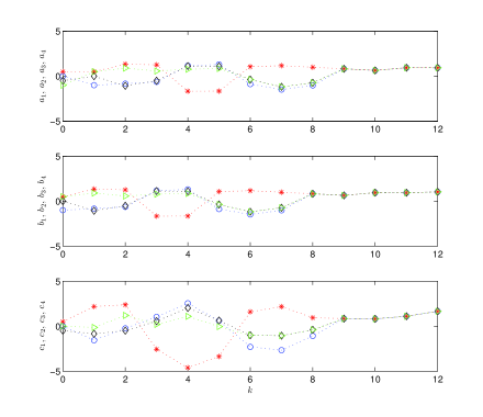
Figure 2: Evolution of states $x_{1}$ (marked $*$), $x_{2}$ (marked $\circ$), $x_{3}$ (marked $\diamond$), and $x_{4}$ (marked $\triangleright$).

7 Notes

The deadbeat interconnection considered in this paper is fixed. A possible relaxation is suggested by the proof of Theorem 4. Namely, deadbeat synchronization would still be achieved with time-varying interconnection $\gamma(k,\,{\mathbf{y}})$ provided that the sets $\mathcal{Y}_{\sigma}$ stayed fixed and the relation $\gamma(k,\,\mathcal{Y}_{\sigma})\subset\mathcal{Y}_{\sigma-1}$ was satisfied at all times $k$. This is very closely related to what we mentioned in Remark 2 regarding the linear array (45). Further generalization in this direction seems nevertheless not to be an easy task.

A practical design problem is how to construct a deadbeat interconnection compatible with a given $(f,\,h)$ pair. A primitive solution to this problem is to select an interconnection that admits a connected graph that is a (directed) tree. In that case, in an array of $q$ systems, $q-1$ of the systems would each be driven by exactly one other system, i.e., for each $i\in\{1,\,2,\,\ldots,\,q-1\}$ we would have $\gamma_{i}({\mathbf{y}})=y_{j}$ for some $j\neq i$, and one system (the root) would be driven by no one, i.e., $\gamma_{q}({\mathbf{y}})=y_{q}$. However, when one starts considering interconnection schemes that include cycles in their graphs, the problem seems to lack an obvious systematic solution.

References

- [1] X. Wang, “Complex networks: topology, dynamics and synchronization,” International Journal of Bifurcation and Chaos, vol. 12, no. 5, pp. 885–916, 2002.
- [2] W. Rugh, Linear System Theory. Second Edition, Prentice Hall, 1996.
- [3] R. Olfati-Saber, J. Fax, and R. Murray, “Consensus and cooperation in networked multi-agent systems,” Proceedings of the IEEE, vol. 95, no. 1, pp. 215–233, 2007.
- [4] L. Moreau, “Stability of multi-agent systems with time-dependent communication links,” IEEE Transactions on Automatic Control, vol. 50, no. 2, pp. 169–182, 2005.
- [5] C. Wu and L. Chua, “Synchronization in an array of linearly coupled dynamical systems,” IEEE Transactions on Circuits and Systems–I: Fundamental Theory and Applications, vol. 42, no. 8, pp. 430–447, 1995.
- [6] L. Pecora and T. Carroll, “Master stability functions for synchronized coupled systems,” Physical Review Letters, vol. 80, no. 10, pp. 2109–2112, 1998.
- [7] S. Tuna, “Synchronizing linear systems via partial-state coupling,” Automatica, vol. 44, no. 8, pp. 2179–2184, 2008.
- [8] S. Glad, “Observability and nonlinear dead beat observers,” in Proc. of the 22nd IEEE Conference on Decision and Control, 1983, pp. 800–802.
- [9] M. Valcher and J. Willems, “Dead beat observer synthesis,” Systems & Control Letters, vol. 37, no. 5, pp. 285–292, 1999.
- [10] S. Tuna, “Deadbeat observer: construction via sets,” IEEE Transactions on Automatic Control, vol. 57, no. 9, pp. 2333–2337, 2012.
- [11] D. Kingston and R. Beard, “Discrete-time average-consensus under switching network topologies,” in Proc. of the American Control Conference, 2006, pp. 3551–3556.
- [12] S. Sundaram and C. Hadjicostis, “Finite-time distributed consensus in graphs with time-invariant topologies,” in Proc. of the American Control Conference, 2007, pp. 711–716.
- [13] A. D. Angeli, R. Genesio, and A. Tesi, “Dead-beat chaos synchronization in discrete-time systems,” IEEE Transactions on Circuits and Systems–I: Fundamental Theory and Applications, vol. 42, no. 1, pp. 54–56, 1995.
- [14] K.-Y. Lian, P. Liu, C.-S. Chiu, and T.-S. Chiang, “Robust dead-beat synchronization and communication for discrete-time chaotic systems,” International Journal of Bifurcation and Chaos, vol. 12, no. 4, pp. 835–846, 2002.
- [15] G. Grassi and D. Miller, “Theory and experimental realization of observer-based discrete-time hyperchaos synchronization,” IEEE Transactions on Circuits and Systems–I: Fundamental Theory and Applications, vol. 49, no. 3, pp. 373–378, 2002.
- [16] ——, “Dead-beat full state hybrid projective synchronization for chaotic maps using a scalar synchronizing signal,” Communications in Nonlinear Science and Numerical Simulation, vol. 17, no. 4, pp. 1824–1830, 2012.
- [17] W. Wonham, “Dynamic observers–geometric theory,” IEEE Transactions on Automatic Control, vol. 15, no. 2, pp. 258–259, 1970.
- [18] ——, Linear Multivariable Control: A Geometric Approach. Third Edition, Springer, 1985.
- [19] A. Rodriguez-Vazquez, J. Huertas, A. Rueda, B. Perez-Verdu, and L. Chua, “Chaos from switched-capacitor circuits: discrete maps,” Proceedings of the IEEE, vol. 75, no. 8, pp. 1090–1106, 1987.