Coherent Adiabatic Spin Control in the Presence of
Charge Noise Using Tailored Pulses

Abstract

We study finite-time Landau-Zener transitions at a singlet-triplet level crossing in a GaAs double quantum dot, both experimentally and theoretically. Sweeps across the anticrossing in the high driving speed limit result in oscillations with a small visibility. Here we demonstrate how to increase the oscillation visibility while keeping sweep times shorter than $T_{2}^{*}$ using a tailored pulse with a detuning dependent level velocity. Our results show an improvement of a factor $\sim 2.9$ for the oscillation visibility. In particular, we were able to obtain a visibility of $\sim 0.5$ for Stückelberg oscillations, which demonstrates the creation of an equally weighted superposition of the qubit states.

The adiabatic theorem of quantum mechanics states that a quantum system will remain in its instantaneous eigenstate if the variation of a dynamical parameter is slow enough on a scale determined by the energy separation from other eigenstates born1928 . However, there are systems for which adiabaticity breaks down resulting in a transition between states. The first result quantifying population change in such a process is due to independent works by Landau, Zener, Stückelberg, and Majorana landau1932 ; zener1932 ; stuckelberg1932 ; majorana1932 . They considered a coupled two-level quantum system whose energies are controlled by a time dependent external parameter, which is defined such that the system exhibits an anticrossing of magnitude $\Delta=2\lambda$ at $t=0$. If the system is prepared in its ground state, $|0\rangle$, at $t=-\infty$ and swept through the anticrossing by modifying the external parameter in such a way that the energy difference is a linear function of time, $\Delta E=\alpha t$, then the probability to remain in $|0\rangle$ at $t=\infty$ (in the diabatic basis) is given by $P_{\mathrm{LZSM}}=\mathrm{e}^{-\frac{2\pi\lambda^{2}}{\hbar\alpha}}$, which is known as the Landau-Zener(-Stückelberg-Majorana) (LZSM) nonadiabatic transition probability. Remarkably, this elegant solution, although valid only in the asymptotic limit for an infinitely long sweep, has demonstrated its accuracy in real physical systems for which the sweep has a finite duration shevchenko2010 .

Another success of the asymptotic formulation resides in an accurate description of LZSM interferometry. If the system is driven back and forth across an anticrossing, it accumulates a Stückelberg phase that gives rise to periodic variations in the transition probability shevchenko2010 . Although the exact accumulated phase can only be calculated by solving the time-dependent Schrödinger equation ribeiro2009 ; ribeiro2010 ; sarkka2011 ; fuchs2011 ; studenikin2012 , a scattering approach assimilating the phase acquired in a single passage to a Stokes phase meyer1989 nicely reproduces experimental results obtained in superconducting qubits oliver2005 , two-electron spin qubits at a singlet ($S$)-triplet ($T_{+}$) anticrossing  petta2010 ; gaudreau2012 , and in nitrogen-vacancy centers in diamond huang2011 .

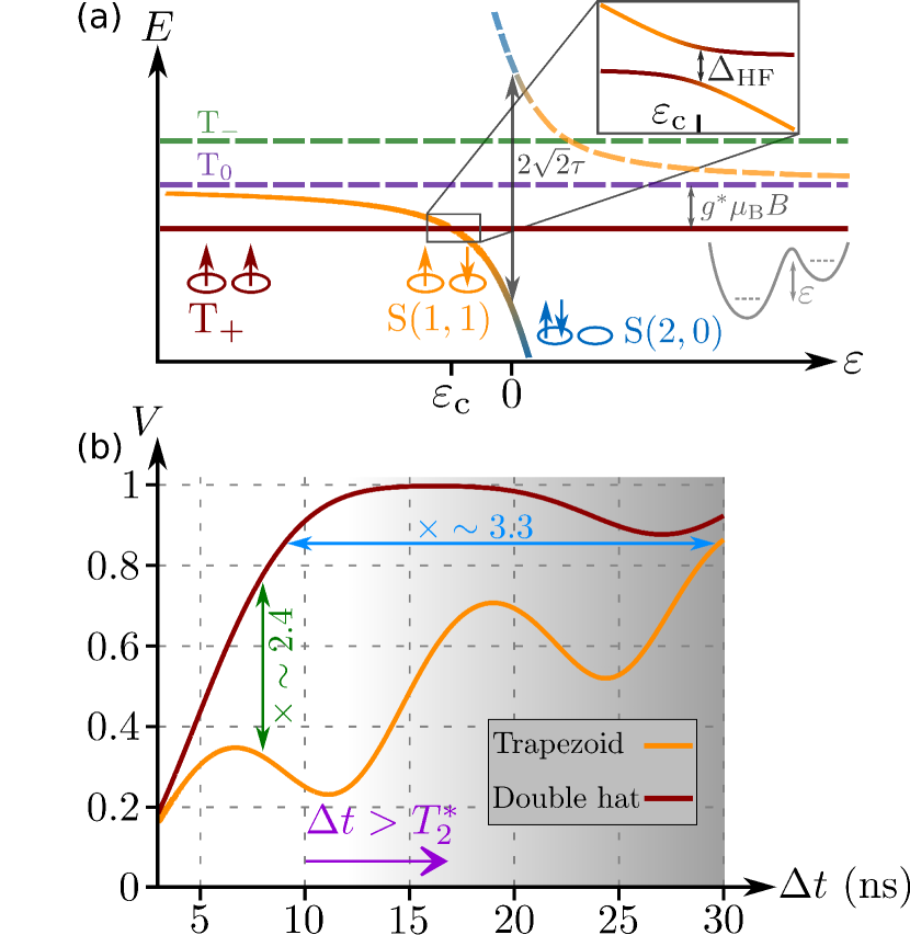
Figure 1: (color online) (a) DQD energy levels as a function of the detuning, $\varepsilon$, near the $(1,1)\leftrightarrow(2,0)$ charge transition. The low energy hybridized singlet state and the triplet $\mathrm{T}_{+}$ form a qubit whose dynamics can be controlled through LZSM interferometry by sweeping the system through the hyperfine mediated anticrossing. (b) Comparison of Stückelberg oscillation visibility $V$ as a function of pulse length, $\Delta t$, for a trapezoid and “double hat” pulse with same maximal amplitude. The oscillation visibility is calculated within a finite-time LZSM model, where it is given by $V=4P_{\mathrm{LZSM}}(1-P_{\mathrm{LZSM}})$. “Double hat” pulses allow for more than a factor of 2 improvement while keeping $\Delta t<T_{2}^{*}$.

Focusing on spin qubits, passage through a $S$-$T_{+}$ anticrossing in the energy level diagram is analogous to a spin-dependent beam splitter petta2010 . There are two major challenges relating to quantum control of such systems. First, in two-electron double quantum dots (DQD), the $S$-$T_{+}$ anticrossing is located near the $(1,1)\leftrightarrow(2,0)$ interdot charge transition, where $(N_{\mathrm{L}},N_{\mathrm{R}})$ refer to the number of electrons in the left and right quantum dots. As a result, the singlet state involved in the spin-dependent anticrossing is a superposition of $(1,1)$ and $(2,0)$ singlet states. Second, the magnitude of the splitting at the level anticrossing is set by transverse hyperfine fields. To achieve LZSM oscillations with 100% visibility, the sweep through the anticrossing would have to be performed on a timescale set by the electron spin decoherence time $T_{\mathrm{2}}^{*}$. As a result, there is a tradeoff between adiabaticity and inhomogeneous dephasing. While there are several studies about dissipative adiabatic passages (see, for instance, ao1989 ; gefen1991 ; wubs2006 ; saito2007 ; nalbach2009 ; lehur2010 ), it remains to be shown how to make a system less sensitive to dissipation while at the same time increasing adiabaticity.

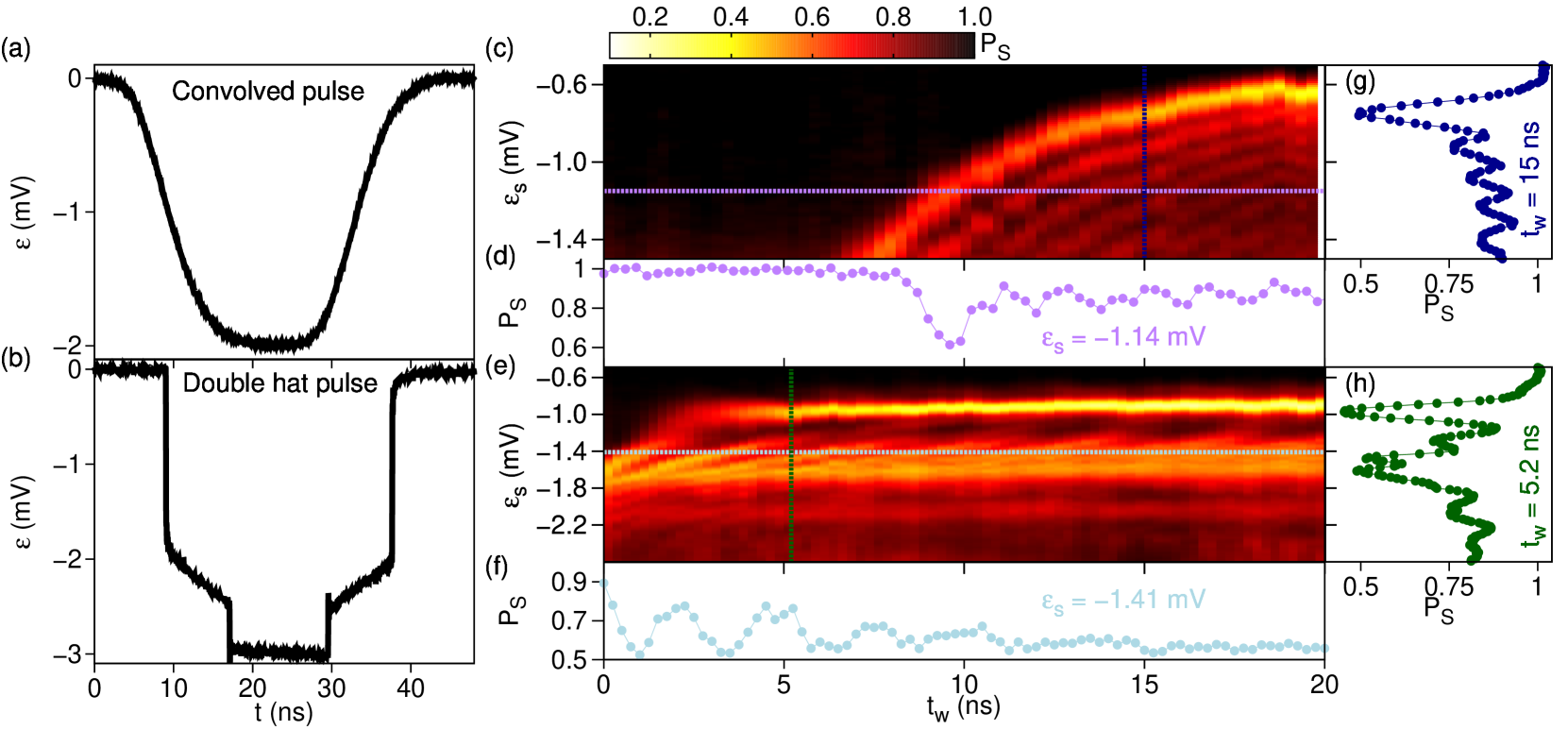
Figure 2: (color online) (a) Convolved pulse obtained by convolving a trapezoid pulse with a Gaussian pulse. (b) “Double hat” pulse with a detuning-dependent level velocity. (c) Singlet return probability $P_{S}$ as a function of $\varepsilon_{\mathrm{s}}$ and $t_{\mathrm{w}}$ for $B=50\,\mathrm{mT}$ using convolved pulses. (d) Trace taken along $\varepsilon_{\mathrm{s}}=-1.14\,\mathrm{mV}$. (e) Singlet return probability $P_{S}$ measured with “double hat” pulses plotted as a function of $\varepsilon_{\mathrm{s}}$ and $t_{\mathrm{w}}$ for $B=55\,\mathrm{mT}$. The results exhibit a high-visibility region corresponding to slow level velocity portion of the “double hat” pulse. (f) Trace taken along $\varepsilon_{\mathrm{s}}=-1.41\,\mathrm{mV}$. This value of $\varepsilon_{\mathrm{s}}$ corresponds to a passage through the anticrossing with the slow level velocity portion of the pulse. (g) and (h) Traces taken along $t_{\mathrm{w}}=15\,\mathrm{ns}$ and $t_{\mathrm{w}}=5.2\,\mathrm{ns}$ for convolved and “double hat” pulses respectively. A comparison between the different traces shows that the “double hat” pulse allows us to achieve higher visibilities, while keeping the total pulse duration below the limit set by $T_{2}^{*}$.

In this Letter, we attempt to reconcile the contradiction between the need for a slow (adiabatic) passage susceptible to dissipation and a fast passage minimizing dissipation effects. Our approach is based on the observation that the biggest population change occurs in the vicinity of the anticrossing. We have developed a multi-ramp pulse sequence that has a detuning dependent level velocity, which we refer to as “double hat” pulse [see Fig. 2(b)]. The slow level velocity portion of the pulse is chosen to coincide with the passage through the $S$-$T_{+}$ anticrossing in order to increase the visibility of the quantum oscillations.

To demonstrate the advantages of “double hat” pulses, we consider a finite-time LZSM model vitanov1996 . In this model, there are three parameters that control the magnitude of $P_{\mathrm{LZSM}}$: the dimensionless coupling $\eta=\lambda/\sqrt{\alpha\hbar}$ and the dimensionless initial and final times $T_{\mathrm{i,f}}=\sqrt{\frac{\alpha}{\hbar}}t_{\mathrm{i,f}}$, where $t_{\mathrm{i,f}}$ are the start and stop times for the pulse relative to $t=0$ defined at the anticrossing. The dependence on $T_{\mathrm{i,f}}$ results in oscillations of $P_{\mathrm{LZSM}}$. In Fig. 1(b), we plot the visibility of Stückelberg oscillations, given by $V=4P_{\mathrm{LZSM}}(1-P_{\mathrm{LZSM}})$ shevchenko2010 , as a function of pulse duration for trapezoid (single ramp) and “double hat” pulses. The duration of the pulse is increased by lowering the level-velocity $\alpha$. For the “double hat” pulse, only the slow level velocity is changed. To be consistent with the regime studied in experiments, we choose $\lambda=50\,\mathrm{neV}$ and energy differences on the order of the Zeeman splitting ($-\Delta E_{\mathrm{i}}=\Delta E_{\mathrm{f}}=2.5\,\mu\mathrm{eV}$). The results demonstrate that “double hat” pulses can improve the oscillation visibility while maintaining a short pulse duration. The oscillation visibility is enhanced because “double hat” pulses allow a passage through the anticrossing with a slower level velocity $\alpha$ as compare to trapezoid pulses. The oscillatory behavior of the results are a consequence of the finite-time LZSM model.

Ideally, one would like the visibility to be unity, which corresponds to the perfect beam splitter limit, $P_{\mathrm{LZSM}}=0.5$. Its achievement would imply the possibility of realizing the Hadamard gate, which is essential to perform certain quantum algorithms (e.g. Shor’s period finding algorithm shor1997 ). Optimization methods to obtain high-fidelity adiabatic passages (i.e. $P_{\mathrm{LZSM}}=0$) have already been studied torosov2011 .

We measure and model LZSM transitions at the $S$-$T_{+}$ anticrossing for finite duration sweeps. Measurements are performed on a GaAs/AlGaAs heterostructure that supports a two-dimensional electron gas located $110\,\mathrm{nm}$ below the surface of the wafer. We use a triple quantum dot depletion gate pattern, where two of the dots are configured in series as a DQD and the third dot serves as a highly sensitive quantum point contact charge detector petta2010 ; som . The DQD is configured in the two-electron regime, where the electrons can either be separated in the $(1,1)$ configuration or localized on a single quantum dot, forming the $(2,0)$ charge state. In this regime, the spin states are the singlets $S(2,0)$ and $S(1,1)$ and the (1,1) triplet states $T_{+}$, $T_{0}$, and $T_{-}$. Interdot tunnel coupling $\tau$ results in hybridization of the charge states at zero detuning with a resulting splitting of magnitude $2\sqrt{2}\tau$ between a ground and excited state singlet, that we respectively denote $S$ and $S^{\prime}$. An external magnetic field is applied perpendicular to the sample, resulting in Zeeman splitting of the triplet states, as depicted in Fig. 1(a). The hyperfine interaction between electron and nuclear spins results in an anticrossing between $S$ and $T_{+}$ located at $\varepsilon_{\mathrm{c}}$. The energy difference at the anticrossing, $\Delta_{\rm HF}$, is set by transverse hyperfine fields taylor2007 .

Simulated interference patterns are obtained by solving the master equation $\dot{\rho}=-\frac{\mathrm{i}}{\hbar}\left[H,\rho\right]+\frac{1}{2}\sum_{i=1}^{3}\left(\left[L_{i}\rho,L_{i}^{{\dagger}}\right]+\left[L_{i},\rho L_{i}^{{\dagger}}\right]\right)$ lindblad1976 . Here, the Hamiltonian $H$ describes the dynamics in the vicinity of the $S$-$T_{+}$ anticrossing and is given by ribeiro2011 ,

$$H(t)=E_{S}(t)|S\rangle\langle S|+E_{T_{+}}|T_{+}\rangle\langle T_{+}|+f(t)\left(|S\rangle\langle T_{+}|+\mathrm{H.c.}\right),$$ (1)

where $E_{S}$ is the unperturbed singlet energy, $E_{T_{+}}=g^{*}\mu_{\mathrm{B}}(B+B_{\mathrm{HF},1}^{z}+B_{\mathrm{HF},2}^{z})$ is the triplet energy, with $g^{*}=-0.44$ the effective Landé $g$-factor, $\mu_{\mathrm{B}}$ the Bohr magneton, $B$ the external magnetic field, and $B_{\mathrm{HF},j}^{z}$ the $z$-component of the hyperfine field in dot $j=1,2$. The effective coupling $f(t)$ between electronic spin states depends on the hyperfine interaction with nuclear spins and on the charge state. It can be written as $f(t)=c(t)\lambda$, with $c(t)$ the time-dependent $(1,1)$ charge amplitude and $\lambda$ the hyperfine matrix element between $S(1,1)$ and $T_{+}$. The Lindblad operators $L_{i}$ are given by $L_{1}=\sqrt{\Gamma_{+}}\sigma_{+}$, $L_{2}=\sqrt{\Gamma_{-}}\sigma_{-}$, and $L_{3}=\sqrt{\Gamma_{\varphi}}\sigma_{z}$. They respectively describe relaxation from excited to ground state and vice versa with rates $\Gamma_{-}=\gamma_{1}(n+1)$ and $\Gamma_{+}=\gamma_{1}n$ due to phonon emission and absorption, with the mean phonon number $n=(\mathrm{e}^{\Delta E/k_{\mathrm{B}}T}-1)^{-1}$ and the spontaneous spin relaxation rate $\gamma_{1}=1/T_{1}$, as well as pure dephasing with a rate $\Gamma_{\varphi}$. A phenomenological model for the rates leads to the relation $\Gamma_{+}+\Gamma_{-}=\gamma_{1}\coth(\Delta E(t)/2k_{\mathrm{B}}T)$, where $\Delta E(t)$ is the energy difference between the instantaneous eigenstates of Eq. (1), $k_{\mathrm{B}}$ is Boltzmann’s constant, and $T$ is the phonon bath temperature ($\sim 10\,\mathrm{mK}$).

We furthermore assume that pure dephasing is mainly due to charge noise when the qubit is in a superposition of $S(2,0)$ and $T_{+}$. Since these two states have different orbital wave functions, they are sensitive to electric fluctuations of the charge background coish2005 ; hu2006 . We thus assume $\Gamma_{\varphi}=\gamma_{2}(1-\left|c(t)\right|^{2})$. The rates $\gamma_{1}$ and $\gamma_{2}$ are free parameters and can be used to fit experimental results. Nuclear spin induced dynamics are obtained by averaging solutions of the master equation over a Gaussian distribution of hyperfine fields khaetskii2002 ; coish2005 , suitable when the thermal energy is larger than nuclear Zeeman energy, $k_{\mathrm{B}}T\gg g_{\mathrm{n}}\mu_{\mathrm{n}}B$, where $g_{\mathrm{n}}$ is the nuclear g-factor and $\mu_{\mathrm{n}}$ is the nuclear magneton. This description of the nuclear state is only valid when its internal dynamics happens on characteristic time scales longer than those of the LZSM driven system (classical approximation). The standard deviation of the distribution of nuclear fields $B_{\mathrm{HF},j}^{i}$ ($i=\{x,y,z\}$, $j=\{1,2\}$) is denoted by $\delta_{j}^{i}$. The singlet energy and charge amplitude coefficient used for our simulations are determined experimentally petta2010 .

We consider two types of pulses to measure the singlet return probability $P_{S}$ petta2010 . Convolved pulses which are obtained by convolving a trapezoid pulse with a finite rise-time of $1.5\,\mathrm{ns}$, a maximal amplitude of $-2\,\mathrm{mV}$ and a variable width $t_{\mathrm{w}}$, with a Gaussian pulse of mean $\mu=0$ and standard deviation $s=3.7\,\mathrm{ns}$ [see Fig. 2(a)]. “Double hat” pulses are tailored to have a detuning-dependent level velocity at the leading and trailing edges of the pulse. The leading edge of the pulse has a level velocity that varies in the sequence fast-slow-fast. The leading edge has a rise time of $0.1\,\mathrm{ns}$ and an amplitude of $-2\,\mathrm{mV}$, which is followed by a slow ramp with a rise time $t_{\mathrm{slow}}=8\,\mathrm{ns}$ and amplitude of $-0.5\,\mathrm{mV}$. A $0.1\,\mathrm{ns}$ rise-time pulse shifts the detuning to its maximal value of $-3\,\mathrm{mV}$, where the detuning is held constant for a time interval $t_{\mathrm{w}}$. The lever-arm conversion between gate voltage and energy is $\sim$0.13 meV/mV. The trailing edge of the pulse is simply the reverse of the leading edge [see Fig. 2(b)]. We present in Fig. 2(c) and (e) $P_{S}$ as a function of final detuning $\varepsilon_{\mathrm{s}}$ and waiting time $t_{\mathrm{w}}$ obtained respectively with convolved pulses for $B=50\,\mathrm{mT}$ and “double hat” pulses for $B=55\,\mathrm{mT}$.

Since $P_{S}$ for convolved pulses exhibits features already discussed in petta2010 , we only discuss the interference pattern obtained with “double hat” pulses. Since the maximal amplitude of these pulses does not depend on $t_{\mathrm{w}}$, we can observe interference fringes that start at $t_{\mathrm{w}}=0\,\mathrm{ns}$, which is a first step for manipulation within $T_{2}^{*}$. More importantly, we notice three distinct regions for detunings smaller than $\varepsilon_{\mathrm{s}}\sim-1\,\mathrm{mV}$, which correspond to different magnitude ranges for $P_{S}$. There is an alternation between regions with $P_{\mathrm{S}}\simeq 1$, $P_{\mathrm{S}}\simeq 0.4\sim 0.9$, and again $P_{\mathrm{S}}\simeq 1$ in correspondence with the different level velocities associated to the “double hat” pulse. A passage through the anticrossing with a slower level velocity improves the oscillation visibility, as we could expect from the earlier considerations within finite-time LZSM theory.

To demonstrate that a high oscillation visibility can be achieved with “double hat” pulses, we compare two different types of traces. First, we compare traces taken for a fixed waiting time. This is equivalent to measuring the visibility of Stückelberg oscillations for a double passage as a function of $\varepsilon_{\mathrm{s}}$. The results are presented in Figs. 2(g) and (h) for convolved pulses and “double hat” pulses. To quantitatively compare the visibility of the coherent oscillations we have to neglect the first interference fringe, which corresponds to a final detuning located at the position of the anticrossing, $\varepsilon_{\mathrm{s}}=\varepsilon_{\mathrm{c}}$, which is strongly affected by relaxation mechanisms (cf. Refs. petta2010 ; ribeiro2011 ). We thus find that the visibility for convolved pulses is $\sim$0.17 and the visibility of “double hat” pulses is $\sim$0.5, which corresponds to an improvement of a factor $\sim$2.9. Second, we present a comparison of traces taken at a fixed value of detuning. This is equivalent to measuring the visibility of Rabi oscillations. The results are presented in Figs. 2(d) and (f) for convolved pulses and “double hat” pulses. Neglecting once more the first oscillation dip, we find, by considering only the first peak and relevant dip, for convolved pulses a visibility of $\sim$0.14 and for “double hat” pulses a visibility of $\sim$0.4. Here, there is an improvement of a factor of $\sim$2.9, which is obtained with $\Delta t\ll T_{2}^{*}$. By considering the first three peaks and dips, i.e. $\Delta t\sim T_{2}^{*}$, we find an improvement of $\sim$2.4. The reduction of visibility is due to nuclear spin dephasing. We expect to obtain improvements in the visibility close to $\sim$2.9 for suitably prepared nuclear states foletti2009 , which exhibit longer decoherence times. The error on the visibility is on the order of the error on $P_{S}$, which we find to be $\sim$7$\%$.

To support our experimental findings, we present in Fig. 3 theory results obtained by using the experimental pulse profiles measured at the output port of the waveform generator. We use $\delta^{x,y,z}_{1,2}=1.00\,\mathrm{mT}$, $\gamma_{1}=10^{5}\,\mathrm{s}^{-1}$, and $\gamma_{2}=10^{8}\,\mathrm{s}^{-1}$. Moreover, since the experimental data are acquired at a high rate with cycles of 5 $\mu$s length, we can observe a build up of nuclear polarization. To take this into account in our model, we allow a nonzero mean for $B_{\mathrm{HF},j}^{i}$. The mean $\xi^{z}_{1,2}\simeq 0.0\,\mathrm{mT}$ for $B_{\mathrm{HF},1,2}^{z}$ can be determined from spin-funnel measurements petta2010 . Since we cannot experimentally determine $\xi_{1,2}^{x,y}$, we have chosen $\xi_{1}^{x,y}=6\,\mathrm{mT}$ and $\xi_{2}^{x,y}=0\,\mathrm{mT}$. Our theory results agree qualitatively with the experiments, as can be seen when comparing interference fringes [see Figs. 3(a) and 2(e)].

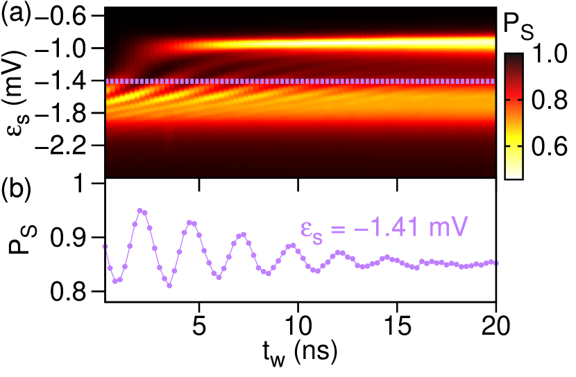
Figure 3: (color online) (a) Theoretical calculations of $P_{S}$ as a function of $t_{\mathrm{w}}$ and $\varepsilon_{\mathrm{s}}$ for “double hat” pulses and $B=55\,\mathrm{mT}$. Theory is in qualitative agreement with the experimental measurements. (b) Trace taken along $\varepsilon_{\mathrm{s}}=-1.41\,\mathrm{mV}$.

Our results indicate that the qubit is not only influenced by nuclear spins, but that there are additional physical mechanisms that determine the oscillation visibility. Here, the contrast is also limited due to the superposition of $S(2,0)$ and $S(1,1)$ ribeiro2011 . First, the weighting of $S(1,1)$ sets the amount of population that can be transferred to $T_{+}$. Second, superpositions of different charge states are susceptible to charge noise, which results in an additional effective spin dephasing mechanism. This dephasing channel directly competes against LZSM tunneling by preventing the qubit from coherently interfering with itself. Spin relaxation also changes the balance of populations, but due to energy scales its effect is weak far from the avoided crossing, where $k_{\mathrm{B}}T\ll\Delta E$.

In conclusion, we have demonstrated how to increase the visibility of quantum oscillations by enhancing the adiabatic passage probability in the presence of dissipation. We have designed a pulse which combines both fast and slow rise-time ramps to minimize dissipation and enhance adiabaticity. By considering a $S$-$T_{+}$ anticrossing, we have shown that it is possible to achieve coherent superposition states with high $T_{+}$ population. In the more general context of LZSM driven spin qubits, this technique allows one to perform more quantum gates within a given decoherence time and achieve higher amplitude rotations in the qubit space without exponentially extending the gate operation times. Our control technique can be further improved by preparing a nuclear spin gradient foletti2009 . This will not only increase $T_{2}^{*}$, but it will also enhance the effective coupling between spin states, thus boosting adiabatic transition probabilities.