The algebraic method in experimental design

Abstract

The algebraic method provides useful techniques to identify models in designs and to understand aliasing of polynomial models. The present note surveys the topic of Gröbner bases in experimental design and then describes the notion of confounding and the algebraic fan of a design. The ideas are illustrated with a variety of design examples ranging from Latin squares to screening designs.

1 Ideals and varieties: introducing algebra

We are familiar with the use of polynomials throughout statistics. For example, much of this handbook is concerned with design for polynomial regression. Thus we have polynomial terms in factors $x_{1},x_{2},\ldots$:

$$x_{1},x_{2}^{2},x_{1}x_{2},\ldots$$

and a second order polynomial response surface in two factors is

$$f(x_{1},x_{2})=\theta_{00}+\theta_{10}x_{1}+\theta_{01}x_{2}+\theta_{20}x_{1}^{2}+\theta_{11}x_{1}x_{2}+\theta_{02}x_{2}^{2}.$$ (1)

The first, but very important, algebraic point is that polynomials are made up of linear combinations of monomials. Consider a set of $k$ factors $x_{1},\ldots,x_{k}$ and non-negative integers $\alpha=(\alpha_{1},\ldots,\alpha_{k})$; a monomial is

$$x^{\alpha}=x_{1}^{\alpha_{1}}x_{2}^{\alpha_{2}}\cdots x_{k}^{\alpha_{k}}.$$

Note that when we use the term polynomial we shall typically mean a polynomial in one or more variables.

A monomial $x^{\alpha}$ can be represented by its exponent vector $\alpha$ and we can list the monomials in a model either directly or by listing a set of exponents. We shall often use the notation $\{x^{\alpha},\alpha\in M\}$, for some set of exponents, $M$. This chapter is largely concerned with the interaction between the choice of a design and the list $M$. We know from classical factorial design that only some models are estimable for a given design and so any such theory must be intimately related to the problem of aliasing and we shall cover this is section 4.

The set of all polynomials over a base field is a ring, so that rings are the basis of the theory. Thus, given a base field $K$ we obtain the ring of polynomials, $R=K[x_{1},\ldots,x_{k}]$ over $K$, which are linear combinations of monomials with coefficients in the base field. Our “$\alpha$” notation allows us to write this compactly as

$$f(x)=\sum_{\alpha\in M}\theta_{\alpha}x^{\alpha},$$

where, as above, $M$ is a finite set of distinct exponents and clearly $f(x)\in R$. For example, the set $M$ for the polynomial model in Equation (1) is $\{(0,0),(1,0),(0,1),(2,0),(1,1),(0,2)\}$.

Given that we have launched into algebra we need to introduce the first two essentials: ideals and varieties. In what follows we present only the basic ideas of the theory, pointing the reader to [11] or [41] for further details.

For a ring $R$ we have special subsets called ideals.

Definition 1

A subset $I\subset R$ is an ideal if for any $f,g\in I$ we have $f+g\in I$ and for any $f\in I$ and $g\in R$ we have $fg\in I$.

The ideal generated by a finite set of polynomials $\{f_{1},\ldots,f_{m}\}$ is the set of all polynomial combinations:

$$\langle f_{1},\ldots,f_{m}\rangle=\{f_{1}g_{1}+\cdots+f_{m}g_{m}:\;g_{1},\ldots,g_{m}\in R\}$$

To have some immediate intuition consider a single point $x$. The set of all polynomials $f$ such $f(x)=0$ is an ideal: since for any polynomial $g(x)$ if $f(x)=0$ we have $g(x)f(x)=0$. In the next section this will be extended to sets of points, namely designs. The Hilbert basis theorem says that any (polynomial) ideal $I$ is finitely generated, i.e. for any ideal we can find a finite collection $f_{1},\ldots,f_{m}\in R$ such that $I\;=\;\langle f_{1},\ldots,f_{m}\rangle$.

We are familiar with linear varieties expressed by setting some linear polynomial function equal to zero. Thus a straight line can be written as the collection of points $(x_{1},x_{2})$ in two dimensions such that $ax_{1}+bx_{2}+c=0,$ for constants $a,b,c$. An algebraic variety is the extension of this concept to simultaneous solutions of a set of polynomial equations.

Definition 2

Let $f_{1},\ldots,f_{m}\in K[x_{1},\ldots,x_{k}]$ be a set of polynomials. The associated affine variety is the solution (also called zero set) of a set of simultaneous equations they define:

$$V(f_{1},\ldots,f_{n})=\{(a_{1},\dots,a_{k})\in K^{k}:f_{i}(a_{1},\ldots,a_{d})=0,\;i=1,\dots,m\}$$

Every affine variety has an associated ideal which we write $I(V)$. It is the set of all polynomial which are zero on the variety:

$$I(V)=\{f\in K[x_{1},\ldots,x_{k}]:f(a_{1},\ldots,a_{k})=0,\;\mbox{for all}\;(a_{1},\ldots,a_{k})\in V\}.$$

What appears to be a straightforward relationship between ideals and varieties is actually very subtle. If we start with polynomials $f_{1},\ldots,f_{m}$ and construct the corresponding variety $V$ and form the ideal $I(V)$, is it true that $I(V)=\langle f_{1},\ldots,f_{m}\rangle$? We can always claim that $\langle f_{1},\ldots,f_{m}\rangle\;\subset\;I(V)$, but the converse may not be true and refer to [11] for a detailed discussion. Fortunately, for a design, the variety is collection of isolated single points, the equivalence holds and we may move freely between ideals and designs.

2 Gröbner bases

Perhaps the most important construction in abstract algebra is that of a quotient. Give two polynomials $f,g\in K[x_{1},\ldots,x_{k}]$ and an ideal $I$ define the equivalence class $f\sim_{I}g$ if and only if $f-g\in I$. The members of the quotient $K[x_{1},\ldots x_{n}]/I$ are the equivalence classes. Since $f_{1}\sim_{I}f_{2}$ and $g_{1}\sim_{I}g_{2}$ imply $f_{1}+g_{1}\sim_{I}f_{1}+g_{2}$ and $f_{1}g_{1}\sim_{I}f_{2}g_{2}$, then $K[x_{1},\ldots x_{n}]/I$ is also a ring. Finding $K[x_{1},\ldots x_{n}]/I$ in a particular case requires a division algorithm. Finding a quotient computationally needs a division algorithm.

2.1 Term orderings

Let us recall division of polynomials in one dimension. If we divide $1+3x+2x^{2}+x^{3}$ by $2+x$ we would obtain the tableau:

$$\begin{array}[]{rll}&\;\;\;\;x^{2}+3\\ x+2&\lx@intercol\hfil\overline{)\;x^{3}+2x^{2}+3x+1}\hfil\lx@intercol\\ &\;\;-x^{3}-2x^{2}\\ \cline{2-3}\cr&&\;\;3x+1\\ &&-3x-6\\ \cline{3-3}\cr&&\lx@intercol\hfil-5\lx@intercol\\ \end{array}$$

giving: $x^{3}+2x^{2}+3x+1=(x^{2}+3)(x+2)-5$. We give this example to remind ourselves that at each stage we need to use the leading term. To obtain leading term we need an ordering. In one dimension the ordering is $1\prec x\prec x^{2}\prec\cdots,$ That is, we order by degree and division is unique. This is generalised to a special total ordering on monomials $\{x^{\alpha}\}$.

Definition 3

A monomial term ordering, $\prec$, is a total ordering of monomials such that $1\prec x^{\alpha}$ for all $\alpha\geq 0$, $\alpha\neq 0$ and, for all $\gamma\geq 0$, $x^{\alpha}\prec x^{\beta}$ implies $x^{\alpha+\gamma}\prec x^{\beta+\gamma}$.

We shall use the term monomial ordering for short. There is a number of standard monomials orderings.

1. Lexicographic ordering, Lex. $x^{\alpha}\prec_{Lex}x^{\beta}$ when (i) $\beta-\alpha\geq 0$ and the leftmost entry of $\beta-\alpha$ is positive.

2. Graded lexicographic ordering, DegLex: $x^{\alpha}\prec_{DegLex}x^{\beta}$ if (i) the degree of $\alpha$ is less than that of $\beta$, $|\alpha|<|\beta|$ and (ii) $\alpha\prec_{Lex}\beta$

3. Reverse lexicographic ordering, DegRevLex: $x^{\alpha}\prec_{DegrevLex}x^{\beta}$ if (i) $|\alpha|<\beta|$ and (ii) $\overline{\alpha}\prec_{Lex}\overline{\beta}$, where the overline means: reverse the entries.

Graded orderings are orderings in which the first comparison between monomials is determined by their total degree. For example, under a graded order, $x_{i}^{2}\succ x_{j}$ for any indeterminates $x_{i},x_{j}$ in the ring $K[x_{1},\ldots,x_{k}]$. The degree lexicographic and degree reverse lexicographic term orders above fall in this class. Contrary to graded orderings, for a lexical ordering in which $x_{i}\succ x_{j}$ then $x_{i}\succ x_{j}^{m}$ for $m=1,2,\ldots$ thus making all powers of $x_{j}$ lower than $x_{i}$.

2.2 Matrix based term orderings

Monomial term orderings can be defined using products with matrices and element-wise comparisons. If the exponents of monomials $x^{\alpha},x^{\beta}$ are considered as row vectors, we say that $x^{\alpha}\prec_{M}x^{\beta}$ if $M\alpha^{T}<M\beta^{T}$, where $M$ is a non-singular matrix and the inequality is tested element-wise starting from the first element. The matrix $M$ above satisfies certain conditions which are stated in the following theorem [41].

Theorem 4

Let $M$ be a full rank matrix of size $k\times k$ such that the first non-zero entry in each column is positive. Then $M$ defines a term ordering in the following sense:

1. For every vector $\alpha\in\mathbb{Z}^{k}_{\geq 0}$ with $\alpha\neq(0,\ldots,0)$ then $(0,\ldots,0)<M\alpha^{T}$ and

2. For any pair of vectors $\alpha,\beta,\gamma\in\mathbb{Z}^{k}_{\geq 0}$ such that $M\alpha^{T}<M\beta^{T}$ then $M(\alpha+\gamma)^{T}<M(\beta+\gamma)^{T}$.

The identity matrix of size $k$ corresponds to the lexical term ordering. Note that the relation between ordering matrices and term orderings is not a one to one. A matrix $M^{\prime}$ defining the same ordering as $M$ can be obtained by multiplying each row of $M$ by a positive constant so for instance the matrix with diagonal $1,2,\ldots,k$ and zeroes elsewhere also defines a lexical term ordering. Usually only integer entries are used for computations although the theory does not preclude using for instance, matrices with rational or real entries [11].

An important case of ordering matrices is that of matrices for graded orderings. Any full rank matrix $M$ in which all elements of the first row are a positive constant defines a graded ordering. The degree lexicographic term ordering is built with a matrix $M$ with all entries one in its first row and the remaining rows are the top $k-1$ rows of an identity matrix. The CoCoA command Use T::=Q[x,y,z], DegLex; creates the same ring and ordering when the matrix and ring are defined with the commands

M:=Mat([[1,1,1],[1,0,0],[0,1,0]]);

Use T::=Q[x,y,z], Ord(M);

The querie xy^2>x^2z; yields output FALSE which means that $xy^{2}\prec x^{2}z$ under the graded lexicographic order in which $x\succ y\succ z$.

The standard ordering in the software system CoCoA is the degree reverse lexicographic (DegRevLex), which is implicit in the following ring definition

Use T::=Q[x,y,z];

xy^2>x^2z;

The output of the querie is TRUE and this is interpreted as $xy^{2}\succ x^{2}z$ under a degree reverse lexicographic term ordering in which $x\succ y\succ z$. Note the reversal of the ordering between the two monomials for the previous graded order.

A more specialized and efficient instance of matrix orderings is produced by a using a single row matrix, in which case we say “ordering vector”. An ordering vector defines only a partial but not a total ordering over $R$. For example the vector $w=(1,1,1)$ naturally produces the ordering $xy^{2}\succ_{w}xz$ because

$$(1,1,1)(1,2,0)^{T}=3>2=(1,1,1)(1,0,1)^{T},$$

yet it cannot distinguish between monomials of the same degree such as $xy^{2}$ and $z^{3}$. However, Gröbner basis are computed over finite sets of monomials rather than over all monomials with exponents in $\mathbb{Z}^{k}_{\geq 0}$. This last fact together with a careful selection of the ordering vector are at the core of the efficient Universal Gröbner bases algorithms [1, 31].

2.3 Monomial ideals and Hilbert series

Now that we have a total ordering any finite set of monomials has a leading term. In particular, since a polynomial, $f$, is based on a finite set of monomials it has a unique leading term. We write it $LT_{\prec}(f)$, or, if $\prec$ is assumed, just $LT(f)$.

A monomial ideal is an ideal generated by monomials. Monomial ideals play a critical part in computational methods for polynomials.

Definition 5

A monomial ideal $I$ is an ideal for which a collection of monomials $f_{1},\ldots,f_{m}$ such that any $g\in I$ can be expressed as a sum

$$g=\sum_{i=1}^{m}g_{i}(x)f_{i}(x).$$

Multiplication of monomials is just achieved by adding exponents:

$$x^{\alpha}x^{\beta}=x^{\alpha+\beta},$$

and $\alpha+\beta$ is in the positive (shorthand for non-negative) “orthant” with corner at $\alpha$. The set of all monomials in a monomial ideal is the union of all positive orthants whose corners are given by the exponent vectors of the generating monomial $f_{1},\ldots,f_{m}$.

For a given monomial ideal, a complete degree by degree description of the monomials inside the ideal or, equivalently, those outside the ideal is given by the Hilbert function and series. Here we only give the basic idea, referring the reader to references [11] and [12] for a full description.

Definition 6

Let $I$ be a monomial ideal in $R$.

1. For all non-negative degrees $j$, the Hilbert function $HF_{I}(j)$ is the number of monomials not in $I$ of total degree $s$.

2. the Hilbert series of $I$ is the formal series $HS_{I}(s)=\sum_{j=0}^{\infty}s^{j}HF(j)$.

The Hilbert series is the generating function of the Hilbert function. Both count monomials which are not in the monomial ideal $I$. In what follows, unless it is required, we omit the subindex referring to the monomial ideal.

Example 1

Consider the ideal $I=\langle x^{3},xy^{2},y^{4}\rangle\subset k[x,y]$. The monomials which do not belong to $I$ are $1,x,x^{2},y,yx,yx^{2},y^{2},y^{3}$, so the Hilbert function equals $1,2,3,2$ for $j=0,1,2,3$ and zero for all $j\geq 4$. The Hilbert series is thus $HS(s)=1+2s+3s^{2}+2s^{3}$.

Note that monomials in the first orthant are counted with the formal series $\sum_{j=0}^{\infty}{j+k-1\choose j}s^{j}$ where $k$ is the number of indeterminates. Then, by substracting the Hilbert series $HS(s)$ from the last expression we have a generating function to count monomials inside $I$. Using two dimensions as in Example 1, the formal series for the firtst orthant is

$$\sum_{j=0}^{\infty}{j+1\choose j}s^{j}=\sum_{j=0}^{\infty}(j+1)s^{j}=\frac{1}{(1-s)^{2}},$$

which counts the monomials in the first quadrant. The generating function for the number of monomials in $I$ for each degree is found by substraction:

$$\frac{1}{(1-s)^{2}}-(1+2s+3s^{2}+2s^{3})=\frac{2s^{3}+s^{4}-2s^{5}}{(1-s)^{2}}.$$

The alternating signs in the polynomial in the numerator are related to inclusion-exclusion rules and although it may seem a simple calculation above, in general determining a simple form of the numerator in this last computation is not a simple task.

Example 2

Consider the monomial ideal in $k[x_{1},\ldots,x_{7}]$ generated by monomials $x_{1}^{2},\ldots,x_{7}^{2}$ and by all pairs $x_{i}x_{j}$, $1\leq i<j\leq 7$. This ideal has Hilbert Function with values $1$ and $7$ for $j=0,1$ and zero for $j\geq 2$ so its Hilbert Series is $HS(s)=1+7s$, i.e. one monomial of degree zero and seven monomials of degree one outside the ideal. The monomials outside this ideal are $1,x_{1},x_{2},x_{3},x_{4},x_{5},x_{6},x_{7}$, which later will be understood as a model for the Plackett-Burman design in Examples 6 and 11. See also first row of Table 4.

2.4 Gröbner bases

Dickson’s Lemma states that, even if we define a monomial ideal with an infinite set of $f_{i}$, we can find a finite set $h_{1},\ldots h_{n}$ such that $I=\langle h_{1},\ldots,h_{k}\rangle$. But there are, in general, many ways to express a ideal $I$ as being generated from a basis $I=\langle f_{1},\dots,f_{m}\rangle$.

Definition 7

Given an ideal $I$ a set $\{g_{1},\ldots g_{m}\}$ is called a Gröbner basis if:

$$\langle LT(g_{1}),\ldots,LT(g_{m})\rangle\;=\;\langle LT(I)\rangle,$$

where $\langle LT(I)\rangle$ is the ideal generated by all the monomials in $I$.

We sometimes refer to $\langle LT(I)\rangle$ as the leading term ideal.

Lemma 8

Any ideal $I$ has a Gröbner basis and any Gröbner basis in the ideal is a basis of the ideal.

Monomial orderings are critical in establishing that for any given monomial ordering, $\prec$, any ideal $I$ has a unique “reduced” Gröbner basis. Given a monomial ordering, $\prec$, and an ideal expressed in terms of the G-basis, $I\;=\;\langle g_{1},\ldots,g_{m}\rangle$ with respect to that monomial ordering any polynomial $f$ has a unique remainder, $r(x)$ with respect the quotient operation $K[x_{1},\ldots,x_{k}]/I$. That is

$$f=\sum_{i=1}^{m}s_{i}(x)g_{i}(x)+r(x)$$ (2)

We call the remainder $r(x)$ the normal form of $f$ with respect to $I$ and write $r(x)=NF(f)$. Or, to stress the fact that it may depend on $\prec$, we write $NF(f,\prec)$.

The division of a polynomial in Equation (2) is the generalization of simple polynomial division such as that of the example shown in Page 2.1, where the result was $s_{1}(x)=x^{2}+3$ with remainder $r=-5$. In other words the normal form of $1+3x+2x^{2}+x^{3}$ with respect to the ideal generated by $g_{1}(x)=2+x$ is $-5$.

Here are some formal definitions.

Definition 9

Given a monomial ordering $\prec$, a polynomial $f=\sum_{\alpha\in L}\theta_{\alpha}x^{\alpha}$ is a normal form with respect to $\prec$ if $x^{\alpha}\notin\langle LT(f)\rangle$ for all $\alpha\in L$.

Lemma 10

Given an ideal $I$ and a monomial ordering $\prec$, for every $f\in K[x_{1},\ldots,x_{k}]$ there is a unique normal form $NF(f)$ such that $f-NF(f)\in I$.

We now need to relate (i) the Gröbner basis, (ii) a division algorithm and (iii) the nature of the normal form. We have partly covered this but let us collect the results together.

1. There are algorithms, which given an ideal, $I$, a monomial ordering $\prec$ and a polynomial $f$ deliver the remainder $r$, in Lemma (8), by successively dividing by the G-basis terms $g_{i},\;i=1,\dots,m$. The best known is the Buchberger algorithm.

2. Suppose the remainder $r(x)=NF(f)=\sum_{\alpha\in L}\theta_{\alpha}x^{\alpha}$, then $\{x^{\alpha},\alpha\in L\}$ is precisely the set of monomials not divisible by any of the leading terms of the G-basis of $I:\;\mbox{LT}(g_{i}),\;i=1,\ldots,m$.

3. The remainder $r(x)=NF(f)$ does not depend on which order the G-basis terms $g_{i}(x)$ are used in the division algorithm.

4. The (maximal) set $\{x^{\alpha},\alpha\in L\},$ which can appear in a remainder $r(x)$ is a basis of the quotient ring, considered as a vector space of functions over $k[x_{1},\ldots,x_{k}]/I$. The terms are linearly independent over $I$:

   $$\sum_{\alpha}\theta_{\alpha}x^{\alpha}\sim_{I}0$$

   implies $\theta_{\alpha}=0$ for all $\alpha\in L$.

2.5 Software tools

All the operations defined above are available on modern computer algebra software. Here is a brief list, the full list is very extensive and extends to nearly all areas of computer algebra, sometimes called computational algebraic geometry: [9]CoCoA, [22], macaulay2, [28] gfan, [23] Singular. A rough list of capabilities relevant to this chapter is as follows.

1. Construction of monomial orderings; the standard ones are usually named and immediately available

2. Ideal operations such as unions, intersections, elimination

3. Buchberger algorithm and modern improvements, quotienting, Normal Forms

4. Special algorithms for ideals of point. We shall use these extensively in our examples

5. Gröbner fan. See section 6

3 Experimental design

We have indicated already that for applications to design we should think of design as lists of points,

$$D=\{x^{(1)},\ldots x^{(n)}\},$$

in $R^{k}$. As algebraic varieties they have associated ideal

$$I(D)=\{f:f(x)=0,\;x\in D\}$$

The use of polynomials to define design is clearly not new. For example a $2^{k}$ full factorial designs give by $\{\pm 1,\ldots,\pm 1\}$ is expressed the solution of the simultaneous equations:

$$\{x_{i}^{2}-1=0,\;i=1,\ldots,k\}.$$

To obtain fractions we impose additional equations: e.g. $x_{1}\ldots x_{k}=1$.

We now give what can loosely be described as the algebraic method in the title of this Chapter. We do this in a step-by-step approach.

1. Choose a design $D$

2. Select a monomial term ordering, $\prec$

3. Compute Gröbner basis for $I(D)$ for given monomial ordering, $\prec$.

4. The quotient ring

   $$K[x_{1},\ldots,x_{k}]/I(D)$$

   of the ring of polynomials $K[x_{1},\ldots,x_{k}]$ in $x_{1},\ldots,x_{k}$ forms is a vector space spanned by a special set of monomials: $x^{\alpha},\alpha\in L$. These are all the monomials not divisible by the leading terms of the G-basis and $|L|=|D|$.

5. The set of multi-indices $L$ has the “order ideal” property: $\alpha\in L$ implies $\beta\in L$ for any $0\leq\beta\leq\alpha$. For example, if $x_{1}^{2}x_{2}$ in the model so is $1,x_{1},x_{2},x_{1}x_{2}$.

6. Any function $y(x)$ on $D$ has a unique polynomial interpolator given by

   $$f(x)=\sum_{\alpha\in L}\theta_{\alpha}x^{\alpha}$$

   such that $y(x)=f(x),\;x\in D$.

7. The cardinality of the design and the quotient basis is the same: $|L|=|D|$.

8. The $X$-matrix is $n\times n$, has full rank $n$ and has rows indexed by the design points and columns indexed by the basis:

   $$X=\{x^{\alpha}\}_{x\in D,\alpha\in L}$$

The implications of the method are considerable. But at its most basic it says that we can always find a saturated polynomial $f(x)$ interpolating data over an arbitrary design $D$.

The shape of the model index set $L$ arising from the order ideal property is important. It is exactly the shape which, in the literature has been called variously: “staircase models”, “hierarchical models”, “well-formulated models”, or “marginality condition”, see [37, 40]. It can be be seen easily from the fact that the multi-index terms given by $L$ are the complement in the non-negative integer orthant of those given by the monomials in the monomial ideal of leading terms: the complement of a union of orthants has the staircase property.

We now give a number of examples.

Example 3

Screening designs. A class of designs for main effect estimation while simultaneously avoiding biases caused by the presence of second order effects and avoid confounding of any pair of second order effects was recently proposed [29]. The authors produced designs of size $n=2k+1$ for different dimensions ranging from $k=4$ up to $k=30$, and their construction is based on folding a certain small fraction of size $k$ of a $3^{k}$ design with levels $-1,0,1$ and then adding the origin. Naturally that after folding and adding the origin, the screening design still remains a special fraction of $3^{k}$ design. Here we consider the designs for $k=7$ and $k=10$ in Table 1.

$\begin{array}[]{rrrrrrr}x_{1}&x_{2}&x_{3}&x_{4}&x_{5}&x_{6}&x_{7}\\ \hline\cr 0&1&-1&1&-1&1&-1\\ 0&-1&1&-1&1&-1&1\\ -1&0&1&-1&1&1&-1\\ 1&0&-1&1&-1&-1&1\\ 1&-1&0&1&1&1&1\\ -1&1&0&-1&-1&-1&-1\\ 1&-1&-1&0&1&-1&-1\\ -1&1&1&0&-1&1&1\\ -1&-1&1&1&0&-1&-1\\ 1&1&-1&-1&0&1&1\\ -1&1&-1&1&1&0&1\\ 1&-1&1&-1&-1&0&-1\\ 1&1&1&1&1&-1&0\\ -1&-1&-1&-1&-1&1&0\\ 0&0&0&0&0&0&0\end{array}$ $\begin{array}[]{rrrrrrrrrr}x_{1}&x_{2}&x_{3}&x_{4}&x_{5}&x_{6}&x_{7}&x_{8}&x_{9}&x_{10}\\ \hline\cr 0&1&1&1&1&1&1&1&1&1\\ 0&-1&-1&-1&-1&-1&-1&-1&-1&-1\\ 1&0&-1&-1&-1&-1&1&1&1&1\\ -1&0&1&1&1&1&-1&-1&-1&-1\\ 1&-1&0&-1&1&1&-1&-1&1&1\\ -1&1&0&1&-1&-1&1&1&-1&-1\\ 1&-1&-1&0&1&1&1&1&-1&-1\\ -1&1&1&0&-1&-1&-1&-1&1&1\\ 1&-1&1&1&0&-1&-1&1&-1&1\\ -1&1&-1&-1&0&1&1&-1&1&-1\\ 1&-1&1&1&-1&0&1&-1&1&-1\\ -1&1&-1&-1&1&0&-1&1&-1&1\\ 1&1&-1&1&-1&1&0&-1&-1&1\\ -1&-1&1&-1&1&-1&0&1&1&-1\\ 1&1&-1&1&1&-1&-1&0&1&-1\\ -1&-1&1&-1&-1&1&1&0&-1&1\\ 1&1&1&-1&-1&1&-1&1&0&-1\\ -1&-1&-1&1&1&-1&1&-1&0&1\\ 1&1&1&-1&1&-1&1&-1&-1&0\\ -1&-1&-1&1&-1&1&-1&1&1&0\\ 0&0&0&0&0&0&0&0&0&0\end{array}$

Table 1: Two screening designs [29].

For $k=7$, the design is obtained by first folding the points 0+-+-+-, -0+-++-, +-0++++, +--0+--, --++0--, -+-++0+, +++++-0 and then adding the origin to total $15$ points. Under the usual degree reverse lexicographic ordering in CoCoA, we identify the model with terms: $1,x_{1},x_{2},x_{3},x_{4},x_{5},x_{6},$ $x_{7},x_{6}^{2},x_{7}^{2},x_{2}x_{7},x_{3}x_{7},x_{4}x_{7},x_{5}x_{7}$ and $x_{6}x_{7}$. We note that use of a graded order allows for the inclusion of all terms of degree one before the addition of terms of second degree, and the total degree of this model (addition of all exponents) is $21$. If a degree lexicographic order is used, the model remains with the same total degree but it interchanges one interaction for a quadratic term: $1,x_{1},x_{2},x_{3},x_{4},x_{5},x_{6},x_{7}$, $x_{5}^{2},x_{6}^{2},x_{7}^{2},x_{5}x_{6},x_{4}x_{7},x_{5}x_{7},x_{6}x_{7}$.

Lexical term orderings work in rather the opposite manner than graded orderings. For a lexical ordering, then selection of terms is concentrated in including all terms with $x_{7}$. As this cannot go further than $1,x_{7},x_{7}^{2}$, then term selection allocates all possible terms including $x_{6}$ until interaction with $x_{6}x_{7}$ appears and term $x_{6}x_{7}^{2}$ can be allocated with $x_{7}$, returning to $x_{6}$ again when required, eventually including terms with $x_{5}$. The model has terms $1,x_{7},x_{7}^{2},x_{6},x_{6}x_{7},x_{6}x_{7}^{2},x_{6}^{2},x_{6}^{2}x_{7},x_{6}^{2}x_{7}^{2},x_{5},x_{5}x_{7},x_{5}x_{6},x_{5}x_{6}x_{7},x_{5}^{2},x_{5}^{2}x_{7}$ and its total degree is $31$.

Varying term orders over all possible orderings is in general a complex and expensive task. In Section 6 we discuss and comment on the whole set of models identified by this seven factor design, when considering all possible term orders.

For $k=10$ the points to be folded are 0+++++++++, +0----++++, +-0-++--++, +--0++++--, +-++0--+-+, +-++-0+-+-, ++-+-+0--+, ++-++--0+-, +++--+-+0- and +++-+-+--0. The standard term ordering in CoCoA was used to identify with this design a model of total degree $30$ with constant, all ten linear terms $x_{1},\ldots,x_{10}$, two quadratic terms $x_{9}^{2},x_{10}^{2}$ and eight double interactions between $x_{10}$ and one of $x_{2},\ldots,x_{9}$. A lexical term ordering produces a model of much higher total degree ($44$) which contains monomials in four factors only ($x_{6},x_{8},x_{9}$ and $x_{10}$): $1,x_{10},x_{10}^{2},x_{9},x_{9}x_{10},x_{9}x_{10}^{2},x_{9}^{2},$ $x_{9}^{2}x_{10}$, $x_{9}^{2}x_{10}^{2},x_{8},x_{8}x_{10},x_{8}x_{9},x_{8}x_{9}x_{10}$, $x_{8}^{2},x_{8}^{2}x_{10},x_{6},x_{6}x_{10}$, $x_{6}x_{9},x_{6}x_{9}x_{10},$ $x_{6}x_{8}$ and $x_{6}x_{8}x_{10}$

Example 4

Response surface design, non-standard. Here we take a $16$-point design which is a $5^{2}$ factorial with all internal points (a $3^{2}$ design) removed:

$$\begin{array}[]{cccc}(2,0)&(2,1)&(2,2)&(1,2)\\ (0,2)&(-1,2)&(-2,2)&(-2,1)\\ (-2,0)&(-2,-1)&(-2,-2)&(-1,-2)\\ (0,-2)&(1,-2)&(2,-2)&(2,-1)\end{array}$$

The design ideal is generated by the following polynomials $x_{2}^{5}-5x_{2}^{3}+4x_{2},x_{1}^{5}-5x_{1}^{3}+4x_{1},x_{1}^{2}x_{2}^{2}-4x_{1}^{2}-4x_{2}^{2}+16$. It can be shown that for any term ordering, the above polynomials form a reduced Gröbner basis and thus the design identifies a single model with terms $1,x_{2},x_{2}^{2},x_{2}^{3},x_{2}^{4},x_{1},x_{1}x_{2},$ $x_{1}x_{2}^{2},x_{1}x_{2}^{3},x_{1}x_{2}^{4},x_{1}^{2},x_{1}^{2}x_{2},x_{1}^{3},$ $x_{1}^{3}x_{2},x_{1}^{4},x_{1}^{4}x_{2}$. In Example 15 a standard response surface design of the central composite type is presented.

Example 5

Regular fraction. Let us take the resolution III in six variables (all main effects estimated independently interaction). In classical notation this has defining contrasts: $\{ABCD,CDEF\}$. Instead of $A,\ldots,F$ we use indeterminates $x_{1},\ldots,x_{6}$ and selecting one of the four blocks expressed we have the ideal

$$\langle x_{1}^{2}-1,x_{2}^{2}-1,x_{3}^{2}-1,x_{4}^{2}-1,x_{5}^{2}-1,x_{6}^{2}-1,x_{1}x_{2}x_{3}x_{4}-1,x_{3}x_{4}x_{5}x_{6}-1\rangle,$$

and setting all polynomials above equal to zero (simultaneously) gives the design. The design ideal is created in the following CoCoA code as the sum of the ideal defining the full factorial design and the ideal defining the desired fraction.

Use T::=Q[x[1..6]];
I:=Ideal([A^2-1|A In Indets()])
   +Ideal(x[1]*x[2]*x[3]*x[4]-1, x[3]*x[4]*x[5]*x[6]-1);

The CoCoA command QuotientBasis(I); gives the quotient basis

[1, x[6], x[5], x[5]x[6], x[4], x[4]x[6], x[3], x[3]x[6], x[2],
 x[2]x[6], x[2]x[4], x[2]x[4]x[6], x[1], x[1]x[6], x[1]x[4],
 x[1]x[4]x[6]]

If the confounding relation is desired for a given monomial, this is computed using the normal form. For example NF(x[2]*x[3]*x[6],I); with output x[1]x[4]x[6] shows that over the design, the term $x_{2}x_{3}x_{6}$ is aliased with $x_{1}x_{4}x_{6}$, equivalently $x_{2}x_{3}x_{6}-x_{1}x_{4}x_{6}\in I(D)$ and thus both terms appear in the same row of the aliasing Table 2. The aliasing table is read row-wise e.g. the first row implies that over the design $1=x_{1}x_{2}x_{3}x_{4}=x_{3}x_{4}x_{5}x_{6}=x_{1}x_{2}x_{5}x_{6}$. Note that the first column of Table 2 corresponds to the quotient basis computed before, and that the row containing the monomial $1$ has the generators of the defining contrast.

$\begin{array}[]{l|lll}1&x_{1}x_{2}x_{3}x_{4}&x_{3}x_{4}x_{5}x_{6}&x_{1}x_{2}x_{5}x_{6}\\ \hline\cr x_{1}&x_{2}x_{3}x_{4}&x_{1}x_{3}x_{4}x_{5}x_{6}&x_{2}x_{5}x_{6}\\ x_{2}&x_{1}x_{3}x_{4}&x_{2}x_{3}x_{4}x_{5}x_{6}&x_{1}x_{5}x_{6}\\ x_{3}&x_{1}x_{2}x_{4}&x_{4}x_{5}x_{6}&x_{1}x_{2}x_{3}x_{5}x_{6}\\ x_{4}&x_{1}x_{2}x_{3}&x_{3}x_{5}x_{6}&x_{1}x_{2}x_{4}x_{5}x_{6}\\ x_{5}&x_{1}x_{2}x_{3}x_{4}x_{5}&x_{3}x_{4}x_{6}&x_{1}x_{2}x_{6}\\ x_{6}&x_{1}x_{2}x_{3}x_{4}x_{6}&x_{3}x_{4}x_{5}&x_{1}x_{2}x_{5}\\ x_{1}x_{4}&x_{2}x_{3}&x_{1}x_{3}x_{5}x_{6}&x_{2}x_{4}x_{5}x_{6}\\ x_{1}x_{6}&x_{2}x_{3}x_{4}x_{6}&x_{1}x_{3}x_{4}x_{5}&x_{2}x_{5}\\ x_{2}x_{4}&x_{1}x_{3}&x_{2}x_{3}x_{5}x_{6}&x_{1}x_{4}x_{5}x_{6}\\ x_{2}x_{6}&x_{1}x_{3}x_{4}x_{6}&x_{2}x_{3}x_{4}x_{5}&x_{1}x_{5}\\ x_{3}x_{6}&x_{1}x_{2}x_{4}x_{6}&x_{4}x_{5}&x_{1}x_{2}x_{3}x_{5}\\ x_{4}x_{6}&x_{1}x_{2}x_{3}x_{6}&x_{3}x_{5}&x_{1}x_{2}x_{4}x_{5}\\ x_{5}x_{6}&x_{1}x_{2}x_{3}x_{4}x_{5}x_{6}&x_{3}x_{4}&x_{1}x_{2}\\ x_{1}x_{4}x_{6}&x_{2}x_{3}x_{6}&x_{1}x_{3}x_{5}&x_{2}x_{4}x_{5}\\ x_{2}x_{4}x_{6}&x_{1}x_{3}x_{6}&x_{2}x_{3}x_{5}&x_{1}x_{4}x_{5}\end{array}$

Table 2: Aliasing table for Example 5.

For regular fractions like this case, the effect of different term orderings in the model means selecting a (possibly) different representative per each row of the aliasing table. If for instance the ring is defined instead with a lexical ordering with the command Use T::=Q[x[1..6]], Lex; then the model terms enter in a lexical fashion. Ten terms $1,x_{2},x_{4},x_{5},x_{6},x_{2}x_{4},$ $x_{2}x_{6},x_{4}x_{6},$ $x_{5}x_{6},x_{2}x_{4}x_{6}$ of the model coincide with the model identified above and six terms $x_{1},x_{3},x_{1}x_{4},x_{1}x_{6},x_{3}x_{6},x_{1}x_{4}x_{6}$ are replaced by $x_{2}x_{5}x_{6},x_{4}x_{5}x_{6},x_{2}x_{4}x_{5}x_{6},x_{2}x_{5},$ $x_{4}x_{5},x_{2}x_{4}x_{5}$. In each case, the replacement monomial is in the same row.

Example 6

Plackett-Burman, PB(8). Consider the Plackett-Burman design [45] with $8$ points in $k=7$ dimensions generated by circular shifts of the generator +++-+-- together with the point +++++++. With the standard ordering in CoCoA, we retrieve the usual first order model: $1,x_{1},x_{2},x_{3},x_{4},x_{5},x_{6},x_{7}$. If a lexical term ordering in which $x_{1}\succ\cdots\succ x_{7}$ is used, the model retrieved is a “slack” model in only four factors with terms $1,x_{4},x_{5},x_{6},x_{7},x_{5}x_{6},x_{5}x_{7},x_{6}x_{7}$.

Example 7

Latin Square. It is a straightforward exercise to code up combinatorial a designs using indicator variables. Let us take as an example the $4\times 4$ Graeco-Latin square derived via the standard Galois field method. The square is

$$\begin{array}[]{cccc}A\alpha&B\beta&C\gamma&D\delta\\ B\gamma&A\delta&D\alpha&C\beta\\ C\delta&D\gamma&A\beta&B\alpha\\ D\beta&C\alpha&B\delta&A\gamma\end{array}$$

Coding up the design with $0-1$ indicators: $x_{ij},\;i,j=1,\ldots,4$, where $i$ indexes the factors rows, columns, and Latin, Greek letters and $j$ the factor “levels”. The design points in this coding are shown in Table 3. Using the a graded lexicographic term ordering in CoCoA, the model identified for the design is

[1, u[4], u[3], u[2], t[4], t[3], t[2], c[4], c[3], c[2], r[4],
 r[3], r[2], t[4]u[4], t[4]u[3], t[4]u[2]]

where the factors labelled u,t identify treatments (Latin and Greek letters) and the factors labelled c,r identify rows and columns of the design. Note the neat decomposition of model terms that coincides with the standard analysis of variance for this orthogonal design:

Source	d.o.f.
Mean	1
u (treatment factor 1)	3
t (treatment factor 2)	3
r (row factor)	3
c (column factor)	3
interaction tu (error)	3
Total	16

The interaction between treatment factors (three terms involving tu above) is often allocated to the error.

$$\begin{array}[]{c}(1,0,0,0,1,0,0,0,1,0,0,0,1,0,0,0)\\ (1,0,0,0,0,1,0,0,0,1,0,0,0,1,0,0)\\ (1,0,0,0,0,0,1,0,0,0,1,0,0,0,1,0)\\ (1,0,0,0,0,0,0,1,0,0,0,1,0,0,0,1)\\ (0,1,0,0,1,0,0,0,0,1,0,0,0,0,1,0)\\ (0,1,0,0,0,1,0,0,1,0,0,0,0,0,0,1)\\ (0,1,0,0,0,0,1,0,0,0,0,1,1,0,0,0)\\ (0,1,0,0,0,0,0,1,0,0,1,0,0,1,0,0)\\ (0,0,1,0,1,0,0,0,0,0,1,0,0,0,0,1)\\ (0,0,1,0,0,1,0,0,0,0,0,1,0,0,1,0)\\ (0,0,1,0,0,0,1,0,1,0,0,0,0,1,0,0)\\ (0,0,1,0,0,0,0,1,0,1,0,0,1,0,0,0)\\ (0,0,0,1,1,0,0,0,0,0,0,1,0,1,0,0)\\ (0,0,0,1,0,1,0,0,0,0,1,0,1,0,0,0)\\ (0,0,0,1,0,0,1,0,0,1,0,0,0,0,0,1)\\ (0,0,0,1,0,0,0,1,1,0,0,0,0,0,1,0)\\ \end{array}$$

Table 3: Design points for Graeco-latin design of Example 7.

Example 8

Balanced Incomplete Block Design, BIBD. Consider the balanced incomplete block design with $n=12$ runs and $t=6$ treatments $t_{1},\ldots,t_{6}$ arranged in $b=6$ blocks of size two $[t_{i},t_{j}]$ for the following pairs $(i,j)$:

$$(1,2),(2,3),(3,4),(4,5),(5,6),(1,6).$$

Using the standard term ordering in CoCoA gives the following model:

[1, t[6], t[5], t[4], t[3], t[2], b[6], b[6]t[6], b[5], b[4], b[3], b[2]]

A similar decomposition to that of Example 7 would allocate the interaction $b_{6}t_{6}$ to the residual error with only one degree of freedom. Under a lexical ordering we retrieve the same model as above. This result is not extremely surprising given the highly restricted range of monomial terms for the model for this design. Thus the biggest influence in selection of model terms is given by the ordering of the indeterminates, also known as initial ordering, see [41].

Example 9

Latin Hypercube Sample. Latin hypercubes [34] are widely used schemes in the design and analysis of computer experiments. The design region is often the hypercube $[0,1]^{k}$ and designs of interest are often those that efficiently cover the design region. Latin hypercubes have at least two clear advantages: univariate projections of the design are uniform and they are simple to generate.

The design $L_{1}$ with points $(0,0,0),(1/5,1,4/5),(2/5,3/5,2/5),$$(3/5,4/5,1/5),$ $(4/5,1/5,1)$ and $(1,2/5,3/5)$ is an example of randomly generated latin hypercube in $k=3$ dimensions and $n=6$ runs. Under the standard term ordering in CoCoA, the design $L_{1}$ identifies the model $1,x_{1},x_{2},x_{3},x_{2}x_{3},x_{3}^{2}$. Experimentally, some latin hypercubes have been found to identify certain types of models which are of minimal degree called “corner cut models”, see [38] also [4]. The design $L_{1}$ belongs to such class, and will be discussed further in Section 6.

A second example of latin hypercube is $L_{2}$ with points $(0,0,4/5),$ $(1/5,1/5,2/5),$ $(2/5,2/5,1)$, $(3/5,3/5,0),(4/5,4/5,3/5)$ and $(1,1,1/5)$. Under the same ordering as above, $L_{2}$ identifies the model $1,x_{2},x_{3},x_{2}x_{3},$ $x_{3}^{2},x_{3}^{3}$.

4 Understanding aliasing

The algebraic method is not only a way of obtaining candidate models but it does, we claim, deliver considerable understanding of the notion of aliasing. Aliasing is close to the idea of equivalence used above to define the quotient operation.

Let $I(D)$ be the design ideal and for two polynomials $f,g$ define

$$f(x)\sim_{D}g(x)$$

to mean $f(x)=g(x),\;x\in D.$ This is equivalent to

$$f(x)-g(x)\in I(D).$$

Again equivalently we have, with respect to a particular monomial ordering $\prec$,

$$NF(f)=NF(g)$$

We call this algebraic aliasing.

However, this is not quite the same as the statistical idea of aliasing. It would be enough that $f=cg$ over the design for some non-zero constant $c$. That is both $f$ and $g$ should not both be in the same regression model. We first need a notation to refer to values of a polynomial $f(x)$ on the design expressed as a vector we write this as $\mbox{supp}_{D}(f(x)).$ Then $f(x)\sim_{D}g(x)$ is equivalent to

$$\mbox{supp}_{D}(f(x))=\mbox{supp}_{D}(g(x))$$

Definition 11

Collections of polynomials $F$ and $G$ are said to be statistically aliased if

$$\mbox{span}\{\mbox{supp}(f),\;f\in F\}=\mbox{span}\{\mbox{supp}(g),\;g\in G\}$$ (3)

and let us write this as

$$F\approx_{D}G$$

Given that $f(x)=\mbox{NF}(f),x\in D$, we can rewrite 3 as

$$\mbox{span}\{\mbox{supp}(NF(f)),\;f\in F\}=\mbox{span}\{\mbox{supp}(NF(g),\;g\in G\}.$$

This means that any aliasing statement is equivalent to one for the normal forms. For $f\in F$, let

$$f=\sum_{\alpha\in L}\theta_{\alpha,f}x^{\alpha},$$

where $L$ is as defined above and depends on the design $D$ and the monomial ordering, $\prec$. Let $\theta_{f}$ be the vector of $\theta_{\alpha,f}$ and define $\theta_{\alpha,g}$, similarly. Then since the matrix $X$ in non-singular, by construction, we have

$$F\approx_{D}G\Leftrightarrow\mbox{span}\{\theta_{f},f\in F\}=\mbox{span}\{\theta_{g},g\in F\}$$

Thus, statistical aliasing can be thought of in two stages: (i) first reduce to expressing each polynomial in $F$ and $G$ to its normal form using the algebra then (ii) compare the coefficient subspaces. In the regular factorial fraction case the normal form of a monomial is itself a monomial, which makes the interpretation easier, but in the general case it is a polynomial.

We can often we can find the alias classes by inspection, once we have the normal form. Consider Example 2 and the monomials $\{x_{1}^{2}x_{2}^{2},x_{1}^{4}x_{2}^{4},x_{1}^{6}x_{2}^{6},$ $x_{1}^{8}x_{2}^{8}\}$. Then, using CoCoA the normal forms are, respectively,

$$\begin{array}[]{c}4x^{2}+4y^{2}-16,\;16x^{4}+16y^{4}-256,\\ 320x^{4}+320y^{4}-256x^{2}-256y^{2}-4096,\\ 5376x^{4}+5376y^{4}-5120x^{2}-5120y^{2}-65536\end{array}$$

We see by inspection that

$$\{1,x_{1}^{2}x_{2}^{2},x_{1}^{4}x_{2}^{4}\}\approx_{D}\{1,x_{1}^{6}x_{2}^{6},x_{1}^{8}x_{2}^{8}\}.$$

The equivalence continues to all $\{1,x_{1}^{2k}x_{2}^{2k},x_{1}^{2k+1}x_{2}^{2k+1}\}$.

To retain the link to classical notation we might say that the collection $\{I,A^{2}B^{2},A^{4}B^{4}\}$ is aliased with the collection $\{I,A^{6}B^{6},A^{8}B^{8}\}$ and we might write

$$\{I,A^{2}B^{2},A^{4}B^{4}\}\approx\{I,A^{6}B^{6},A^{8}B^{8}\}$$

This arises because $A^{2}B^{2}\approx A^{2}+B^{2}-4I$ and $A^{4}B^{4}\approx A^{4}+B^{4}-16$, and both the reduced forms are estimable.

In this example odd terms also pair up. The normal forms of $\{x_{1}^{3}x_{2}^{3},x_{1}^{5}x_{2}^{5},x_{1}^{7},$ $x_{2}^{7},x_{1}^{9}x_{2}^{9}\}$ are respectively

$$\begin{array}[]{c}4x^{3}y+4xy^{3}-16xy,\;80x^{3}y+80xy^{3}-384xy\\ 1344x^{3}y+1344xy^{3}-6656xy,\;21760x^{3}y+21760xy^{3}-108544xy\end{array}$$

So that $\{1,x_{1}^{3}x_{2}^{3},x_{1}^{5}x_{2}^{5}\}\approx\{1,x_{1}^{7}x_{2}^{7},x_{1}^{9}x_{2}^{9}\},$ and so on, and in classical notation: $\{I,A^{3}B^{3},A^{5}B^{5}\}\approx\{I,A^{7}B^{7},A^{9}B^{9}\}$.

5 Indicator functions and orthogonality

At times it is convenient to see the design $D$ as a subset of a full factorial design $\mathcal{N}$. This is most usual when we start with some basic design, such as a full factorial, and consider a fraction. We saw such a fraction in the last subsection. In this case an algebraic description of the fraction is via an indicator function: $F_{D}$, rather than a G-basis. The design ideal of $D$ is unique, what changes are the generating equations we choose to describe it. These encode different information on $D$.

An indicator function is a single additional function which we add to the generators of the ideal of the full factorial design to form the ideal of $D$. We can write the last example as

$$I(D)=\langle x_{1}^{2}-1,x_{2}^{2}-1,x_{3}^{2}-1,x_{1}x_{2}x_{3}+1\rangle.$$

The first three terms form the $G$-basis of the full factorial $\{(\pm 1,\pm 1,\pm 1)\}$.

From the equation $f(x_{1},x_{2},x_{3})=x_{1}x_{2}x_{3}+1=0$ we can deduce the indicator functions of $D$ in $\mathcal{N}$ as $g(x_{1},x_{2},x_{3})=\frac{2-f}{2}=\frac{1}{2}(-x_{1}x_{2}x_{3}+1)$. This takes the value $1$ on the design and $0$ on $\mathcal{N}\setminus D$. Then, on $D$:

$$x_{1}x_{2}x_{3}+1=0\Leftrightarrow g(x_{1},x_{2},x_{3})=1$$

More generally let $\mathcal{N}$ be the basic, starting design which is not necessarily a full factorial design, and let $D\subset\mathcal{N}$ be a fraction. Fix a monomial order and, via the $I(\mathcal{N})$, construct a vector space basis for interpolation over $\mathcal{N}$. Then the indicator function of $D$ interpolates the $0,1$ values as required:

$$g(x)=\left\{\begin{array}[]{l}1,\;x\in D\\ 0,\;x\in\mathcal{N}\backslash D\\ \end{array}\right.$$

In the example above, there is only one basis for interpolation, being $\mathcal{N}$ a full factorial design: $\{x_{1}^{\alpha_{1}}x_{2}^{\alpha_{2}}x_{3}^{\alpha_{3}}:\alpha_{i}\in\{0,1\}\textrm{ for }i=1,2,3\}$ and the indicator function involves only the terms for $\alpha=(0,0,0)$ and $\alpha=(1,1,1)$.

The coefficients of the indicator functions expressed over the interpolation basis embed information on the ’geometric/combinatoric’ properties of the fraction. We exemplify this in the binary case where $\mathcal{N}$ is the $2^{d}$ with coding $\{-1,1\}$ [20]. For factors with mixed levels a coding with complex numbers is needed [43].

Two (square-free) monomials $x^{\alpha},x^{\beta}$ are said to be are said to be orthogonal over $D\subset\mathcal{N}$ if the corresponding columns in the $X$-matrix are orthogonal:

$$\sum_{x\in D^{\prime}}x^{\alpha}x^{\beta}=\sum_{x\in D^{\prime}}x^{\alpha+\beta}=0.$$

We can express this in terms of the indicator function over $\{-1,1\}^{d}$ and write

$$\sum_{x\in\mathcal{N}}x^{\alpha+\beta}g(x)=0$$

because $g(x)=0$ over $\mathcal{N}\setminus D$ and $g(x)=1$ over $D$. In the example above we want to check that the two-way factors are not orthogonal to the one-way factor. Indeed

$$\sum_{x\in\mathcal{N}}x_{1}x_{2}x_{3}\frac{2-x_{1}x_{2}x_{3}}{2}=\sum_{x\in\mathcal{N}}\frac{2x_{1}x_{2}x_{3}-1}{2}=\sum_{x\in\mathcal{N}}x_{1}x_{2}x_{3}-4=-4\neq 0$$

because $x_{1}^{2}=1$ over $\mathcal{N}$. It is no coincidence that the coefficient of $x_{1}x_{2}x_{3}$ in the indicator function is not zero. Out of the zero coefficients of $g$ one can deduce the orthogonal (monomial) functions over $D$.

A very practical advantage of the indicator function is that we can take union and intersections of design rather easily by using Boolean type operations over $D$:

$$g_{D_{1}\cap D_{2}}=g_{D_{1}}g_{D_{2}},\;g_{D_{1}\cup D_{2}}=g_{D_{1}}+g_{D_{2}}-g_{D_{1}}g_{D_{2}}.$$

Again the zero coefficients of the normal form of $g_{D_{1}\cap D_{2}}$ and $g_{D_{1}\cup D_{2}}$ over the interpolation monomial basis of $\mathcal{N}$ are informative of the geometry of the intersection and union design.

6 Fans, state polytopes and linear aberration

The computations of Gröbner basis and model identification with Gröbner basis described in Sections 2 and 3 depend upon the term ordering selected. Setting a fixed term order allows the experimenter to put preference over terms which will be identified by the model, for instance a graded ordering will include as many terms of order one as possible factors before adding terms of second degree in the model. In other instances, the experimenter might be interested in exploring the range of all models identifiable by the design using algebraic techniques. For example this would allow assessment of design properties like estimation capacity [7, 8] or the minimal linear aberration of the design [4] and its general case of non-linear aberration [3]. Fan computations have been applied among others, to industrial experiments [27] and systems biology [15].

Some figures of this Section were generated with gfan and computations were performed with CoCoA and gfan [9, 28].

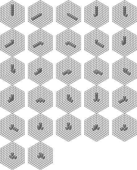
Figure 1: Algebraic fan of design $L_{1}$ of Example 9.

6.1 The algebraic fan of a design

Given a design ideal $I(D)$ and ranging over all possible term orderings, we have a collection of reduced Gröbner bases for $I(D)$. A crucial fact is that despite the infinite number of different term orderings (excluding the trivial case of one dimension), this collection of bases has always a finite number of distinct elements [35]. Associated to this collection of Gröbner bases there is a collection of polyhedral cones, called the Gröbner fan, and we term the algebraic fan of the design to the collection of different bases for the quotient ring $R/I(D)$. Note that the algebraic fan is effectively, a collection of saturated models.

For some relatively simple designs, such as factorial designs, the algebraic fan has only a single model. The general class of designs with a single model is called echelon designs [41]. However, at present, computation of the algebraic fan of a design remains an expensive computation. Reverse search techniques are at the core of state-of-the-art software gfan [28]. However, other approaches remain under investigation, such as the polynomial-time approach based on partial orderings, operations with matrices and zonotopes [1, 31]. The well known link between Gröbner basis calculations and linear algebra operations for zero dimensional ideals (i.e. design ideals) allows these methodologies to be efficient [13, 30]

Example 10

(Continuation of Example 9) The collection of all models identifiable by the design $L_{1}$ (algebraic fan of $L_{1}$) was computed. Design $L_{1}$ identifies $27$ different models which can be classified in only six types of models, up to permutations of variables: $1,x_{1},x_{1}^{2},x_{1}^{3},x_{1}^{4},x_{1}^{5}$ (3 models); $1,x_{1},x_{1}^{2},x_{1}^{3},x_{1}^{4},x_{2}$ (6 models); $1,x_{1},x_{1}^{2},x_{1}^{3},x_{2},x_{1}x_{2}$ (6 models); $1,x_{1},x_{2},x_{1}^{2},x_{1}x_{2},x_{2}^{2}$ (3 models); $1,x_{1},x_{2},x_{3},x_{1}^{2},x_{1}^{3}$ (3 models) and $1,x_{1},x_{2},x_{3},x_{1}^{2},x_{1}x_{2}$ (6 models).

We say that this fan has a complete combinatorial structure, meaning that each class of models is closed under permutations of indeterminates, e.g. if the model $1,x_{1},x_{1}^{2},x_{1}^{3},x_{1}^{4},x_{1}^{5}$ is in the fan, so are the models $1,x_{2},x_{2}^{2},x_{2}^{3},x_{2}^{4},x_{2}^{5}$ and $1,x_{3},x_{3}^{2},$ $x_{3}^{3},x_{3}^{4},x_{3}^{5}$, obtained by permuting indeterminates.

The algebraic fan of $L_{1}$ is depicted in Figure 1, where each model is represented as a staircase diagram, with indeterminates $x_{1},x_{2},x_{3}$ along axes and one small box for each monomial term. The models are presented by classes following the order described above (row-wise from top left). For instance, the first diagram shows the model $1,x_{3},x_{3}^{2},x_{3}^{3},x_{3}^{4},x_{3}^{5}$, the second is $1,x_{1},x_{1}^{2},x_{1}^{3},x_{1}^{4},x_{1}^{5}$ and so on.

Now we turn our attention to the other latin hypercube $L_{2}$. From the design coordinates we note that this design has complete confounding between $x_{1}$ and $x_{2}$ and we should expect a much more limited collection of models. Indeed this design identifies only $11$ models which are depicted in Figure 2. Only one of the models contains terms with $x_{1}$ (first from left in second row); while the rest of the models have monomials in $x_{2}$ and $x_{3}$. The models can be classified in three classes, only one of which is closed under permutation of indeterminates (shown in the left column in Figure 2).

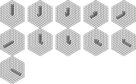
Figure 2: Algebraic fan of design $L_{2}$ of Example 9.

Simplicial	Degree	$HS(s)$	Class size	Example
complex				Vertex/Model
	$7$	$1+7s$	$1^{*}$	$(1,1,1,1,1,1,1)$
				$1,x_{1},x_{2},x_{3},x_{4},x_{5},x_{6},x_{7}$
	$8$	$1+6s+s^{2}$	$105^{*}$	$(1,1,1,2,1,2,0)$
				$1,x_{1},x_{2},x_{3},x_{4},x_{5},x_{6},x_{4}x_{6}$
	$9$	$1+5s+2s^{2}$	$420$∗	$(0,1,2,2,3,0,1)$
				$1,x_{2},x_{4},x_{3},x_{5},x_{7},x_{4}x_{5},x_{3}x_{5}$
	$10$	$1+4s+3s^{2}$	$84$∗	$(1,3,0,3,0,3,0)$
				$1,x_{1},x_{2},x_{4},x_{6},x_{2}x_{4},x_{2}x_{6},x_{4}x_{6}$

Table 4: Summary of the algebraic fan of the Plackett-Burman design.

Example 11

(Continuation of Example 6) In total there are $610$ different hierachical models identifiable by the Plackett-Burman design. Those models belong to $4$ different classes, only two of which are generated by all permutations of factors. Note that as the design has only two levels in each factor, the models identified by this design are all multilinear. The lowest total degree of models is $7$, and the largest total degree is $10$. See Table 4 for details and examples for each class, where the sign ^∗ refers to a class which is closed under permutation of indeterminates. The Hilbert Series $HS(s)$ has been included to describe model terms degree by degree in each class.

Class	Total	$HS(s)$	Class	Example
	degree		size	Vertex/Model
I	$26$	$\begin{array}[]{l}1+6s+7s^{2}\\ +2s^{3}\end{array}$	$24$	$(5,5,6,2,1,7)$
				$1,x_{1},x_{2},x_{3},x_{4},x_{5},x_{6},x_{1}x_{2},x_{1}x_{3},x_{1}x_{6},$
				$x_{2}x_{3},x_{2}x_{6},x_{3}x_{6},x_{4}x_{6},x_{1}x_{3}x_{6},x_{2}x_{3}x_{6}$
II			$24$	$(7,1,4,4,3,7)$
				$1,x_{1},x_{2},x_{3},x_{4},x_{5},x_{6},x_{1}x_{3},x_{1}x_{4},x_{1}x_{5},$
				$x_{1}x_{6},x_{3}x_{6},x_{4}x_{6},x_{5}x_{6},x_{1}x_{3}x_{6},x_{1}x_{4}x_{6}$
III			$24$	$(4,4,6,2,2,8)$
				$1,x_{1},x_{2},x_{3},x_{4},x_{5},x_{6},x_{1}x_{3},x_{1}x_{6},x_{2}x_{3},$
				$x_{2}x_{6},x_{3}x_{6},x_{4}x_{6},x_{5}x_{6},x_{1}x_{3}x_{6},x_{2}x_{3}x_{6}$
IV	$28$	$\begin{array}[]{l}1+5s+7s^{2}\\ +3s^{3}\end{array}$	$24$	$(6,6,2,6,0,8)$
				$1,x_{1},x_{2},x_{3},x_{4},x_{6},x_{1}x_{2},x_{1}x_{4},x_{1}x_{6},x_{2}x_{4},$
				$x_{2}x_{6},x_{3}x_{6},x_{4}x_{6},x_{1}x_{2}x_{6},x_{1}x_{4}x_{6},x_{2}x_{4}x_{6}$
V			$24$	$(4,8,0,8,4,4)$
				$1,x_{1},x_{2},x_{4},x_{5},x_{6},x_{1}x_{2},x_{1}x_{4},x_{2}x_{4},x_{2}x_{5},$
				$x_{2}x_{6},x_{4}x_{5},x_{4}x_{6},x_{1}x_{2}x_{4},x_{2}x_{4}x_{5},x_{2}x_{4}x_{6}$
VI	$32$	$\begin{array}[]{l}1+4s+6s^{2}\\ +4s^{3}+s^{4}\end{array}$	$12$	$(8,0,8,8,0,8)$
				$1,x_{1},x_{3},x_{4},x_{6},x_{1}x_{3},x_{1}x_{4},x_{1}x_{6},x_{3}x_{4},x_{3}x_{6},$
				$x_{4}x_{6},x_{1}x_{3}x_{4},x_{1}x_{4}x_{6},x_{1}x_{3}x_{6},x_{3}x_{4}x_{6},x_{1}x_{3}x_{4}x_{6}$

Table 5: Summary of the algebraic fan of regular fraction $2^{6-2}$.

Example 12

(Continuation of example 5) The fan of the regular $2^{6-2}$ fraction with generators $\{ABCD,CDEF\}$ is of relatively modest size: $132$ models which belong to six equivalence classes whose size range from $12$ to $24$. Models range from total degree $26$ to $32$ and none of the equivalence classes is closed under permutation of indeterminates, which is not entirely surprising given the regularity of the design. Despite this apparent fan simplicity, this six classes share only three different total degrees and Hilbert functions. For instance, three different model classes share the same total degree $26$ while other two different model classes have total degree $28$. Table 5 shows a summary of the fan computations for this design, and Figure 3 shows simplicial representation of models in each class (vertices refer to single factors, edges to two factor interactions and so on).

Figure 3: Depiction of simplicial models for fan classes I-VI (left to right), design $2^{6-2}$.

Example 13

(Continuation of Example 3) The algebraic fan of the screening design for seven factors $k=7$ and $n=15$ runs is a complicated and large object which nevertheless exhibits in some instances combinatorial symmetry. The design identifies $18368$ staircase models which can be classified in $25$ equivalence classes. The class sizes range from $7$ to $2520$, while total degree of models range from $21$ to $31$. Six equivalence classes are closed under permutation of indeterminates, and this includes the classes of models identified by degree lexicographic ($420$ models) and by degree reverse lexicographic ($210$ models); examples of models for each ordering were computed in Example 3. Other $2$ equivalence classes are almost closed, each can be paired with a other small equivalence class.

6.2 State polytope and linear aberration

The state polytope of $I(D)$ is a geometric object which is associated with the Gröbner fan of $I(D)$ [2, 35]. The state polytope is constructed as the convex hull of state vectors, and each state vector is built from a model in the algebraic fan by simply adding the exponents of the model. Aside from a constant, indeed each state vector is the centroid of the staircase diagram represented by the model and thus the state polytope is the convex hull of all those centroids.

The state polytope of $I(D)$ encodes information by variables about the total degree of each model in the fan of design $D$. A simple argument of linear programming shows that models in the algebraic fan are those that minimise a simple linear cost function on the weighted degree of the model. This is the idea of linear aberration defined in [4]. This concept has been generalised to nonlinear cost functions [3, 13].

Example 14

For the latin hypercube design $L_{1}$, the state polytope of its design ideal is built with state vectors for each of the $27$ models ennumerated in Example 10. For instance, the model $1,x_{1},x_{1}^{2},x_{1}^{3},x_{1}^{4},x_{1}^{5}$ has state vector

$$(0,0,0)+(1,0,0)+(2,0,0)+\ldots+(5,0,0)=(15,0,0)$$

and as the other two models in this class are created by permutations of variables, the same action is performed on the state vectors so for this class we have three vectors: $(15,0,0),(0,15,0)$ and $(0,0,15)$. A similar construction and arguments are used for each model in the fan of $L_{1}$ and we have $6$ vectors with permutations of each of $(10,1,0)$, $(7,2,0)$ and $(4,2,1)$ ; three permutations for each of $(4,4,0)$ and $(6,1,1)$.

There is a special type of polynomial models which are of minimal weighted degree. These models are termed corner cut staircases [38], as their exponents can be separated by their complement by a single hyperplane. The properties of corner cut staircases and their cardinality have been studied in literature [10, 48].

A design that identifies all corner cut models is termed a generic design, and automatically a generic design is of minimal linear aberration [4]. The collection of models identified by design $L_{1}$ (of Examples 9, 10 and 14) is the set of all corner cut staircases for $k=3$, $n=6$ and thus $L_{1}$ is a generic design. State polytopes associated with corner cuts and generic designs were described in [36].

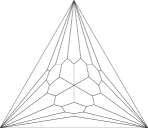
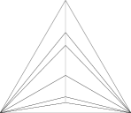
Figure 4: Gröbner fan for designs $L_{1}$ (left) and $L_{2}$ (right) of Example 9.

In addition to information about degrees of models in the fan, the state polytope also encodes information to compute Gröbner bases. To each vertex of the state polytope, a normal cone is associated [49]. The collection of all those cones is precisely the Gröbner fan of $I(D)$, in the sense that the interior of each full dimensional cone contains ordering vectors necessary to compute the Gröbner basis (and identify the model) for the corresponding vertex.

In Figure 4, cones in the fan of state polytopes for designs $L_{1}$ and $L_{2}$ are depicted. As in each case the tridimensional cones form a partition of the first orthant, the figures show a slice of the cones when intersected with the standard simplex. The diagram for design $L_{1}$ (left panel) shows $27$ cells, one for each model. The central symmetry of the diagram corresponds to symmetry of models under permutation of indeterminates. Ordering vectors taken from the same cell will yield the same vertex (and corresponding model). Now in contrast with generic design $L_{1}$, design $L_{2}$ produced the right panel in Figure 4. The diagram shows still some symmetry, but not central symmetry. This symmetry reflects the range of models computed for $L_{2}$ in Example 10, where only $11$ models are identifiable by $L_{2}$, and ten models are in terms of $x_{2}$ and $x_{3}$. The following example illustrates changes in the fan by addition of one point to the design.

Example 15

Response surface design, central composite design. Consider the central composite design design in three factors built with axial points at distance $\sqrt{2}$ and a full factorial design with points at levels $\pm 1$. If no point is added to the origin, this design has $14$ points and a combinatorial algebraic fan with $6$ models. The models in the fan belong to only two classes, one with monomials $1,z,z^{2},z^{3},z^{4},y,yz,yz^{2},y^{2},$ $x,xz,xz^{2},xy,xyz$ and the other class replaces $z^{4}$ by $x^{2}$ above. Addition of the origin to the previous design has a simplification effect in the fan, reducing to only $3$ models, while it remains combinatorial. The only class of models is created by the list above together with the monomial $x^{2}$. See depictions of both fans in Figure 5, with the left panel depicting design without origin and the right panel after adding the origin.

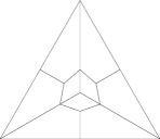
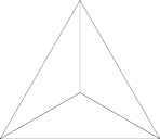
Figure 5: Algebraic fan of central composite designs in Example 15.

7 Other topics and references

The algebraic method in the form discussed here can be said to have started started with [44], [14], [16] and the basic ideas were presented in the monograph [41]. A short review is [47]. More extensive work on the computation of universal Gröbner basis with zonotopes appears in [1]. Applications to designs appear in mixtures [21] and [32]. Industrial applications were performed, perhaps surprisingly early: [27] [42].

For an excellent summary of the wider work in the field of Algebraic statistics: see [17]. One important topic omitted from this chapter, but important for conducting exact conditional test for contingency tables via Markov Chain Monte Carlo is the construction of Markov bases; see [26] [25] [24] [5]. Important applications to biology, which continue, are covered in [39]. Related and of considerable recent interest is the algebraic study of boundary Exponential models: [46] [6] [18].

Recent work showed the link between minimal aberration models and the border description of models in terms of Betti numbers of monomial ideals [33], see also extensive references in that paper.

References

- [1] Babson, E., Onn, S. and Thomas, R. The Hilbert zonotope and a polynomial time algorithm for universal Gröbner bases. Adv. Appl. Math., 30(3):529–544, 2003.
- [2] D. Bayer and I. Morrison. Standard bases and geometric invariant theory. I. Initial ideals and state polytopes. J. Symb. Comput., 6(2-3):209–217, 1988.
- [3] Berstein, Y., Lee, J., Maruri-Aguilar, H., Onn, S., Riccomagno, E., Weismantel, R. and Wynn, H. Nonlinear matroid optimization and experimental design. SIAM J. Discrete Math., 22(3): 901–919.
- [4] Bernstein, Y., Maruri-Aguilar, H., Onn, S., Riccomagno, E. and Wynn, H. Minimal average degree aberration and the state polytope for experimental designs. Ann. Inst. Stat. Math., 62:673–698, 2010.
- [5] Carlini, E. and Rapallo, F. A class of statistical models to weaken independence in two-way contingency tables. Metrika, 73(1), 1-22, 2011.
- [6] Cena, A. and Pistone, G. Exponential statistical manifold. Ann. Inst. Statist. Math., 59(1), 27-56, 2007.
- [7] Chen, H. H. and Cheng, C.-S. (2004). Aberration, estimation capacity and estimation index. Statistica Sinica, 14(1):203–215.
- [8] Cheng, C.-S. and Mukerjee, R. (1998). Regular fractional factorial designs with minimum aberration and maximum estimation capacity. The Annals of Statistics, 26(6):2289–2300.
- [9] CoCoATeam. CoCoA: a system for doing Computations in Commutative Algebra. Available at http://cocoa.dima.unige.it, 2009.
- [10] Corteel, S., Rémond, G., Schaeffer, G. and Thomas, H. The number of plane corner cuts. Adv. Appl. Math., 23(1): 49–53, 1999.
- [11] Cox, D., Little, J. & O’Shea, D., Ideals, Varieties, and Algorithms, 1996, Springer-Verlag (New York, Second Edition).
- [12] Cox, D., Little, J. and O Shea, D. Using Algebraic Geometry, 1998, Springer-Verlag, New York-Berlin-Heidelberg.
- [13] De Loera, J. A., Haws, D. C., Lee, J. and O’Hair, A. Computation in multicriteria matroid optimization. ACM J. Exp. Algorithmics, 14, 1.8:1–1.8:33, 2009.
- [14] Diaconis, P. and Sturmfels, B. Algebraic algorithms for sampling from conditional distributions. Ann. Statist., 26(1), 1998.
- [15] Dimitrova, E. S., Jarrah, A. S., Laubenbacher, R. and Stigler, B. A Gröbner fan method for biochemical network modeling. ISSAC 2007, 122–126.
- [16] Dinwoodie, I. H. The Diaconis-Sturmfels algorithm and rules of succession. Bernoulli, 4(3), 401-410, 1998.
- [17] Drton, M., Sturmfels, B. and Sullivant, S. Lectures on algebraic statistics. Oberwolfach Seminars, Volume 39. Birkhäuser Verlag, Basel, 2009.
- [18] Drton, M. and Sullivant, S. Algebraic statistical models. Statist. Sinica, 17(4), 1273-1297, 2007.
- [19] Evangelaras, H. and Koukouvinos, C. A comparison between the Gröbner bases approach and hidden projection properties in factorial designs. Computational Statistics & Data Analysis, 50(1):77–88, 2006.
- [20] Fontana, R., Pistone, G., and Rogantin, Maria. Classification of two-level factorial fractions. J. Statist. Plann. Inference, 87(1): 149–172.
- [21] Giglio, B., Wynn, H.P. and Riccomagno, E. Gröbner basis methods in mixture experiments and generalisations. In Optimum design 2000 (Cardiff), Nonconvex Optim. Appl., 51, 33-44, Kluwer Acad. Publ., Dordrecht, 2001.
- [22] Grayson, D. R. and Stillman, M. E. Macaulay2, a software system for research in algebraic geometry. Available at http://www.math.uiuc.edu/Macaulay2/, 2009.
- [23] Greuel, G.M., Pfister, G., Schönemann, H.: Singular 3-1-0 — A computer algebra system for polynomial computations (2009). Http://www.singular.uni-kl.de
- [24] Hara, H. and Takemura, A. Connecting tables with zero-one entries by a subset of a Markov basis. In Algebraic methods in statistics and probability II, Contemp. Math., 516, 199-213, 2010.
- [25] Hara, H., Sei, T. and Takemura, A. Hierarchical subspace models for contingency tables. J. Multivariate Anal., 103, 19-34, 2012.
- [26] Hara, H., Aoki, S. and Takemura, A. Minimal and minimal invariant Markov bases of decomposable models for contingency tables. Bernoulli, 16(1), 208-233, 2010.
- [27] Holliday, T., Pistone, G., Riccomagno, E. and Wynn, H.P. The application of computational algebraic geometry to the analysis of designed experiments: a case study. Comput. Statist., 14(2), 213-231, 1999.
- [28] Jensen, A. N.. Gfan, a software system for Gröbner fans and tropical varieties. Available at http://home.imf.au.dk/jensen/software/gfan/gfan.html.
- [29] Jones, B., Nachtsheim, C.J. A class of three-level designs for definitive screening in the presence of second-order effects. Technometrics, 43(1): 1–15, 2011.
- [30] Lundqvist, S. Vector space bases associated to vanishing ideals of points. J. Pure Appl. Algebra 214(4): 309–321, 2010.
- [31] Maruri-Aguilar, H. Universal Gröbner bases for designs of experiments. Rend. Istit. Mat. Univ. Trieste, 37(1-2):95–119, 2006.
- [32] Maruri-Aguilar, H., Notari, R. and Riccomagno, E. On the description and identifiability analysis of experiments with mixtures. Statist. Sinica, 17(4):1417–1440, 2007.
- [33] H. Maruri-Aguilar, E. Sáenz-de Cabezón, and H. Wynn. Betti numbers of polynomial hierarchical models for experimental designs. Ann. Math. Art. Int., 2011. In print.
- [34] McKay, M. D., Beckman, R. J., and Conover, W. J. (1979). A comparison of three methods for selecting values of input variables in the analysis of output from a computer code. Technometrics, 21(2):239–245.
- [35] Mora, T. and Robbiano, L. The Gröbner fan of an ideal. J. Symb. Comput., 6(2-3), 1988.
- [36] Müller, I. Corner cuts and their polytopes. Beiträge Algebra Geom., 44(2):323-333, 2003.
- [37] Nelder, J. A. A reformulation of linear models. J. Roy. Statist. Soc. Ser. A, 140(1):48–76, 1977. With discussion.
- [38] Onn, S. and Sturmfels, B. (1999). Cutting corners. Advances in Applied Mathematics, 23(1):29–48.
- [39] Pachter, L. and Sturmfels, B. Algebraic statistics for computational biology. Cambridge Univ. Press, New York, 2005.
- [40] Peixoto, J.L., A property of well-formulated polynomial regression models, 1990, The American Statistician 44(1), 26-30.
- [41] Pistone, G., Riccomagno, E. and Wynn, H.P. Algebraic Statistics, volume 89 of Monographs on Statistics and Applied Probability. Chapman & Hall/CRC, Boca Raton, 2001.
- [42] Pistone, G. and Riccomagno, E. and Wynn, H.P. Gröbner basis methods for structuring and analysing complex industrial experiments. Int. J. Rel. Qual. Saf. Eng., 7(4), 285-300, 2000.
- [43] Pistone, G. and Rogantin, M.-P. Indicator function and complex coding for mixed fractional factorial designs. J. Statist. Plann. Inference, 138(3):787–802, 2008.
- [44] Pistone, G. and Wynn, H.P. Generalised confounding with Gröbner bases. Biometrika, 83:656–666, 1996.
- [45] Plackett, R.L., Burman, J.P. The design of optimum multifactorial experiments, 1946, 305-325.
- [46] Rauh, J., Kahle, T. and Ay, N. Support sets in exponential families and oriented matroid theory. Internat. J. Approx. Reason., 52(5), 613-626, 2011.
- [47] E. Riccomagno. A short history of algebraic statistics. Metrika, 69(2-3):397–418, 2009.
- [48] Wagner, U. On the number of corner cuts. Adv. Appl. Math., 9(2):152–161.
- [49] Ziegler, G.M. Lectures on polytopes. Graduate Texts in Mathematics, Vol 152. Springer-Verlag, New York, 1995.