Ab Initio Simulations of Hot, Dense Methane During Shock Experiments

Methane is one of the most abundant chemical species in the universe, with the vast majority of our solar system’s share being locked away in the interiors of the giant planets hubbard-81 . While recent work has suggested that icy components of the cores of gas giants such as Jupiter and Saturn are likely to be dissolved into the surrounding hydrogen WilsonMilitzer2012 ; WilsonMilitzer2012b , the ice giants Uranus and Neptune likely contain a significant amount of methane at pressures ranging from 20 to 80 GPa and 2000 to 8000 K. Extrasolar planets in the ice giant mass regime are now known to be extremely common throughout the universe borucki . This motivates our need for a greater understanding of the behaviour of this important material in this specific range of pressures and temperatures.

Dynamic shock experiments Hicks2006 ; Knudson2009 combined with static precompression KananiLee2006 ; MH08 ; jeanloz2007 have the potential to probe the behavior of methane at pressures and temperatures in ice giant interiors but these experiments are challenging and their interpretation often not straightforward Spaulding2012 ; Militzer2012 . There exists a long tradition of first-principles simulation predicting the outcome of past MC00 ; Mi01 ; Knudson2009 ; Mi09 and future Mi06 shock experiments and providing an interpretation on the atomistic level for the thermodynamic changes that were observed Mi03 . Here we use density functional molecular dynamics (DFT-MD) simulations to characterize the properties of dense, hot methane and identify a molecular, a polymeric, and a plasma state. From the computed equation of state, we predict the shock Hugoniot curves for different initial densities in order to guide future shock wave experiments with precompressed samples.

The high pressure, high temperature behavior of methane has previously been probed experimentally and theoretically across a range of conditions, revealing a complex chemical behavior characterized by the conversion of methane into higher hydrocarbons and eventually diamond as pressure is increased. Laser heated diamond anvil cell (LHDAC) studies by Benedetti et al. benedetti showed the presence of polymeric hydrocarbons and diamond at pressures between 10 and 50 GPa and temperatures of about 2000 to 3000 K. More recently, a LHDAC experiment by Hirai et al. hirai found evidence of the formation of carbon-carbon bonds occurring above 1100 K and 10 GPa, including the formation of diamond above 3000 K. Gas gun shock wave experiments by Nellis  et al. nellis achieved pressures of 20 to 60 GPa and produced results that were interpreted as the formation of carbon nanoparticles. Radousky et al. radousky previously carried out shock experiments at lower pressures that did not reach the dissociation regime.

Ancilotto et al. ancilotto performed DFT-MD simulations that followed the predicted isentropes of the intermediate layers of Uranus and Neptune. At 100 GPa and 4000 K methane was found to dissociate into a mixture of hydrocarbons. At 300 GPa and 5000 K it became apparent that carbon-carbon bonds were favored with increasing pressure. Recent DFT-MD simulations with free energies derived from the velocity autocorrelation function by Spanu et al. spanu predicted that higher hydrocarbons than methane are energetically favored at temperature-pressure conditions between 1000 and 2000 K and at 4 GPa and above. Static zero-kelvin calculations by Gao et al. gao predicted methane to decompose into ethane at 95 GPa, butane at 158 GPa and diamond at 287 GPa. Goldman et al. goldman computed shock Hugoniot curves for the molecular regime of methane up to 50 GPa. Better agreement with experiments was obtained by approximately including quantum corrections to the classical motion. The vibrational spectrum for each atomic species was derived from DFT-MD simulations and the internal energy was corrected by assuming each atom has six harmonic degrees of freedom. This approach is exact for a harmonic solid but its validity remains to be more carefully evaluated for molecular fluids.

Laser and magnetically driven shock experiments Hicks2006 ; Knudson2009 now allow multi-megabar pressures to be obtained routinely, however the lack of independent control of the pressure and temperature variables makes the direct study of planetary interior conditions difficult MH08 ; jeanloz2007 . For any given starting material, the pressure and temperature conditions of the shocked material are uniquely determined by the shock velocity. Conservation of mass, momentum and energy across the shock front lead to the Hugoniot relation zeldovich ,

$$H=(E-E_{0})+\frac{1}{2}(P+P_{0})(V-V_{0})=0,$$ (1)

relating the final values of the internal energy, $E$, pressure, $P$, and volume, $V$, to the corresponding values $E_{0},P_{0}$, and $V_{0}$ for the initial state of the material. While shocks launched into materials at ambient conditions allow extremely high pressures to be reached, a large part comes from the thermal pressure and the density is often only about 4 times higher than the initial value Mi06 . The resulting shock temperatures are significantly higher than those along the planetary isentrope. Static precompression of the sample, however, shifts the Hugoniot curves to higher densities allowing higher pressures to be explored for given temperature. Precompressed shock experiments on methane are thus highly desirable as a means of exploring the pressure-temperature conditions of interest to planetary science.

In this article, we present theoretically computed methane shock Hugoniot curves corresponding to initial densities ranging from 0.35 to 0.70 g cm^-3 and temperatures up to 75 000 K. We use DFT-MD simulations to determine equations of state of methane at relevant temperature-pressure conditions, compute the equation of state, and analyze the atomistic and electronic structure of the hot, dense fluid in order to make predictions for future shock measurements using methane.

I Computational methods

All DFT-MD simulations in this article were performed with the Vienna Ab Initio Simulation Package (VASP) vasp . Wavefunctions were expanded in a plane wave basis with an energy cutoff of 900 eV, with core electrons represented by pseudopotentials of the projector augmented wave type paw . Exchange-correlation effects were approximated with the functional of Perdew, Burke, and Ernzerhof pbe . Each simulation cell consisted of 27 methane molecules in a cubic cell with temperature controlled by a Nose-Hoover thermostat. The Brillouin zone was sampled with $\Gamma$ point only in order to invest the available computer time into a simulation cell with more atoms. Electronic excitations were taken into account using Fermi-Dirac smearing mermin .

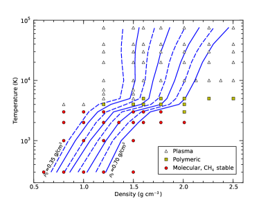
Figure 1: Methane shock Hugioniot curves showing temperature as a function of density for different initial densities, $\rho_{0}=\{0.35,0.40,0.45,0.50,0.55,0.60,0.65,0.70\}$. The symbols show the density and temperature conditions of our DFT-MD simulations that either stayed molecular, or reached a polymeric or plasma state.

Simulations were undertaken at 79 different temperature-density conditions as shown in Fig. 1, chosen in order to encompass the Hugoniot curves for methane at initial densities ranging from 0.35$-$0.70 g cm^-3. Temperatures ranged from 300 to 75 000 K and pressures from 3 to 1100 GPa. Each simulation lasted between 1 and 2 ps, and in some cases up to 8 ps. Almost all simulations used an MD time step of 0.2 fs. Initially, we performed a few simulations with a time step of 0.4 fs at lower temperatures but reduced the timestep as we explore higher temperature and densities. Our tests showed that the computed thermodynamic functions at lower temperatures agreed within error bars with the results obtained with the shorter time step.

II Results

The pressure and internal energy computed from DFT-MD simulations at various densities and temperatures are given in Tab. 1 in the online supplemental information. Any initial transient behavior was removed from the trajectories before the thermodynamic averages were computed. Hugoniot curves were calculated by linear interpolation of the Hugoniot function, $H$, in Eq. (1) as a function of temperature and pressure. Figure 1 shows temperature as a function of density along the Hugoniot curves generated for each of the eight initial densities, $\rho_{0}$. Several features are immediately apparent. As might be expected, precompression allows higher densities to be reached at any given temperature. Each Hugoniot curve can be divided into three segments. Up to 3000 K, one finds the temperature to increase linearly with density. In our simulations, the methane molecules remained intact. At a temperature of approximately 4000–5000 K, a plateau is reached where density increases rapidly without a corresponding increase in temperature. Our simulations show the system entering into a polymeric regime where the methane molecules spontaneously dissociate to form long hydrocarbon chains that dissociate and reform rapidly. We will demonstrate this regime to be metallic, which implies a high electrical conductivity and reflectivity should be detected during a shock experiments.

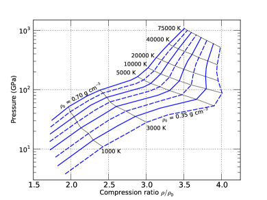
Figure 2: The pressure as function of the compression ratio, $\rho/\rho_{0}$, along the shock Hugoniot curves from Fig. 1 for different initial densities, $\rho_{0}$.

In the third regime, the temperature on the Hugoniot curve again increases rapidly as the system assumes a plasma state where many ionic species exist for a very short time. The slope of the curve significantly depends on the initial density. For a small degree of precompressions, density on the Hugoniot curve does not increase in the plasma regime because the sample has already been 4-fold compressed. For a high degree of precompression, density of the Hugoniot curve keeps increasing in the plasma regime because the theoretical high temperature limit of 4-fold compression has not yet been reached. This is confirmed in Fig. 2 where we plotted the shock pressure as a function of compression ratio, $\rho/\rho_{0}$. The highest compression ratio of 4.0 is obtained for 10 000 K and the lowest initial density. In general, the compression ratio is controlled by the excitation of internal degrees of freedom that increase the compression and interaction effects that act to reduce it Mi06 . The strength of the interactions increases with density, which explains why the compression ratio decreases when the sample is precompressed.

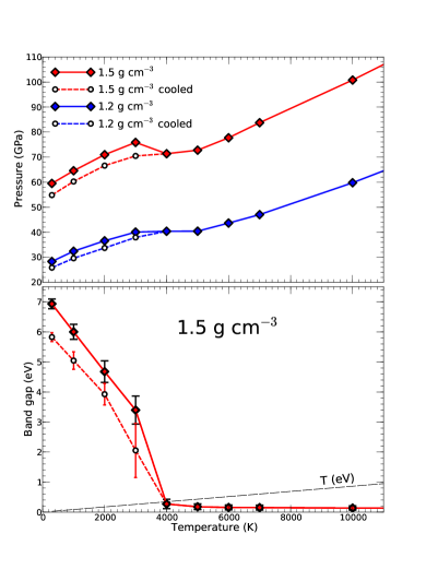
Figure 3: The upper panel shows the pressure-temperature relation of CH₄ DFT-MD simulations that have been heated (filled symbols) and of samples that have been cooled (open symbols) from a polymeric state at 4000 K. The lower panel shows the corresponding electronic gap bands and its variance during the MD simulations. For $T\geq 4000\,$K, the average band gap that is less than the temperature (dashed line), which implies that the polymeric and the plasma state are good electrical conductors.

We now focus on characterizing the polymeric state that gives rise to the predicted increase in shock compression at 4000 K. Fig. 3 shows a linear increase of pressure with temperature as long as the methane molecules remain intact. When the molecules dissociate at 4000 K, the pressure reaches a plateau at 40 GPa for 1.2 g cm^-3 before it rises gradually above 5000 K when the system turns into a plasma. For a higher density of 1.5 g cm^-3, one observes a significant drop in pressure when molecules disassociate that resembles the behavior of molecular hydrogen. DFT-MD simulations of hydrogen also show that the dissociation of molecules leads to a region with $\partial P/\partial T|_{V}<0$ at high density because hydrogen atoms can also be packed more efficiently than molecules MHVTB ; Morales2010 .

When the simulations are cooled from 4000 K, the system remained in a polymeric state that exhibits a lower pressure than the original simulations with methane. This confirms the free energy calculations in Ref. spanu that showed the polymeric state to be thermodynamically more stable.

In Fig. 3, we also plot the electronic band gap averaged over the trajectory at different temperatures. From 300 to 3000 K, the system remains in an insulating state with a gap of 3 eV or larger. When the system transforms into the polymeric state at 4000 K, the gap drops to a value close to zero and remains small as the temperature is increased further and the system transforms into a plasma. One may conclude that this insulator-to-metal transition is driven by the disorder that the dissociation introduced into the fluid and resembles recent findings for dense helium StixrudeJeanloz08 ; Mi09 where the motion of the nuclei also led to a band gap closure at unexpectedly low pressures.

If the band gap energy is comparable to $k_{B}T$, the system becomes a good electrical conductor and its optical reflectivity increases. Since reflectivity measurements under shock conditions celliers2010 have now become well established, the transformation into a polymeric state at 4000 K can directly be detected with experiments. However, if this transformation already occurs at lower temperature, the polymeric transition will be more difficult to detect with optical measurements alone because Fig. 3 shows that a band gap opens back up as the polymeric state is cooled.

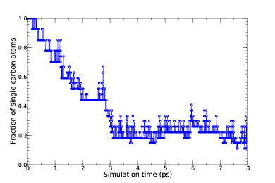
Figure 4: Evolution of fraction of single carbon atoms during the MD simulation at 4000 K and 1.2 g cm^-3. The decrease measures how many methane molecules polymerize to form long carbon chains, which is illustrated in Fig. 5.

We now study the transformation into the polymeric state in more detail by analyzing the clusters in the fluid. Most simply, one can detect different polymerization reactions by analyzing the carbon atoms only. Using a distance cut-off of 1.8 Å, we determined how many C_n clusters were present in each configuration along different MD trajectories. Methane molecules are classified as C₁ clusters in this approach. Figure 4 shows a drop in the fraction of C₁ clusters as the system at 4000 K and 1.2 g cm^-3 transforms into a polymeric state over the course of approximately of 3 ps.

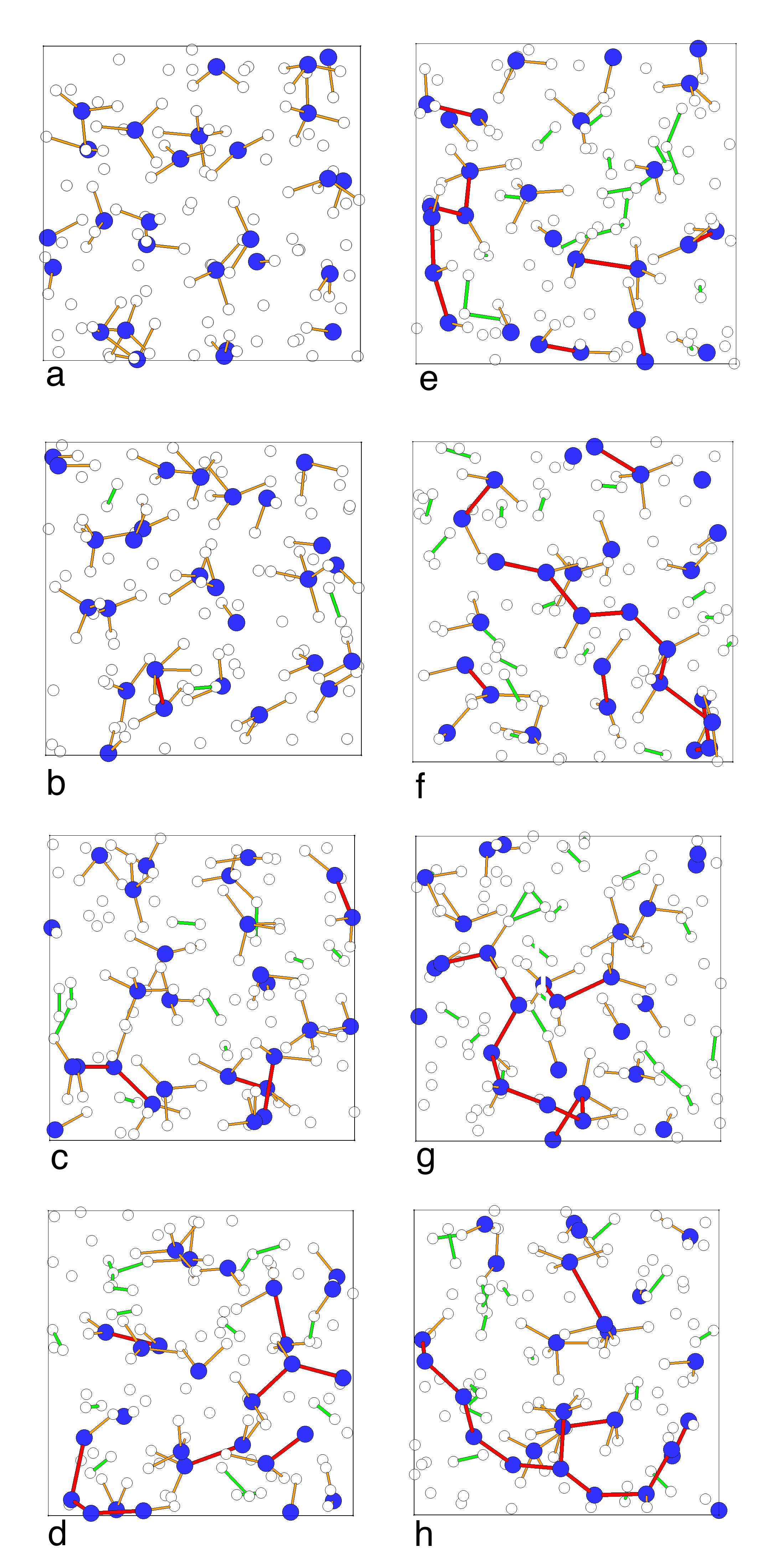
Figure 5: (color online) Series of snapshots from MD simulations at 4000 K and 1.2 g cm^-3. The large and small spheres depict the carbon and hydrogen atoms, respectively. The C-C, C-H, and H-H bonds are illustrated by dark thick lines, thin lines, and thick light lines, respectively. Panel (a) depicts the initial configuration with 27 CH₄ molecules. (b) shows the formation of the first ethane molecule. Some H₂ molecules have also formed. (c) and (d) show the first C₃ and C₄ chains that formed. (e-g) illustrate linear C₆, C₇, and C₁₀ chains while (h) shows a 12 atoms chain with one branching point.

In Fig. 5, we show a series of snap shots from the same DFT-MD simulation in order to illustrate how hydrocarbons chain of increasing length are formed. As soon as the first C₂ cluster occurs, we also find molecular hydrogen to be present. This resembles typical dehydrogenation reactions such as $n$CH${}_{4}\to$ C_nH${}_{2n+2}+(n-1)$H₂ that were also analyzed in spanu . This implies that molecular hydrogen may be expelled as a methane rich system transforms into a polymeric state.

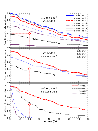
Figure 6: Cumulative lifetime distribution of carbon clusters of different sizes at various densities and temperatures. The square in the upper panel shows that, on average, 26% of the carbon atoms are bound in carbon clusters with 20 atoms or more that exit for at least 25 fs. Similarly, the open circle illustrates that 66% of the atoms are bound in clusters with 5 atoms or more. Simulations were characterized as polymeric if at least 40% of the atoms were bound in clusters with 5 atoms or more that existed for at least 20 fs (diamond symbol).

In the polymeric regime, the system is primarily composed of different types of hydrocarbon chains but each chain exists only for a limited time before it decomposes and new chains are formed. Every chemical bond has a finite lifetime, which makes it similar to a plasma, but many chains are present in every given snap shot, which may be a unique feature of carbon rich fluids and makes the distinction from a typical plasma state worthwhile.

We computed the lifetime of each C_n cluster in the DFT-MD simulation, neglecting any information that may be stored in the position of the hydrogen atoms. In Fig. 6 we plot the fraction of carbon atoms that were bound in clusters of different size and lifetimes. The plot is cumulative in two respects. The curve for cluster size $n$ presents the average fraction of carbon atoms in clusters with at least $n$ atoms with a lifetime at least as long as the lifetime specified on the ordinate. By definition, the C${}_{1}(t)$ curve approaches 1 for small $t$. It is surprising, however, that, in simulations at 2.0 g cm^-3 and 4000 K, 26% of all carbon atoms were bound in clusters with 20 atoms or more that existed for at least 25 fs.

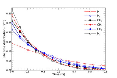
Figure 7: Lifetime distribution of plasma species at 20 000 K and 1.5 g cm^-3.

We characterized a simulation as polymeric if, on average, at least 40% of the carbon atoms were at any given time bound in clusters with 5 atoms or more with lifetimes of at least 20 fs. All simulations with cluster size 5 curves that fall above the diamond symbol in Fig. 6 are then considered to be polymeric. The minimum cluster size of 5 atoms distinguishes the polymeric state from simulations with stable methane molecules while the lifetime constraint distinguishes it from a plasma where one finds many small ionic species that exist for less than 1 fs. Figure 7 shows a typical lifetime distribution of the most common ionic species that we obtained from a cluster analysis that includes C and H atoms.

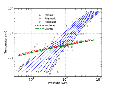
Figure 8: Pressure as a function of temperature along the shock Hugoniot curves from Fig. 1 for different initial densities, $\rho_{0}$. Shown for reference are the Uranus and Neptune isentropes redmer .

This cluster analysis allowed us to characterize all simulations in Figs. 1 and 8 as either molecular, polymeric, or as a plasma. It is important to note that the classification refers to the state reached in our picosecond-timescale DFT-MD simulations and, in case where we find the CH₄ molecules to be stable, this may not necessarily be the thermodynamic ground state. If all methane molecule remained stable in our simulation we described the state as molecular, even though our cooled simulations did not revert back to a molecular state. Previous studies (Ref. spanu ) showed the polymeric state is thermodynamically favorable for pressures above 4 GPa.

In Fig. 8, we plot temperature as a function of pressure along each of the Hugoniot curves. There is a noticeable change in the slope at approximately 4000–5000 K as the the Hugoniot curves enter the polymeric regime and then the plasma state, but it is not as pronounced as indicated in the temperature-density plot in Fig. 1.

We also included in Fig. 8 the isentropes for Uranus and Neptune that were approximately determined using DFT-MD simulations of only H₂O redmer . These indicate that precompressed shock experiments with initial densities from 0.35 to 0.70 g cm^-3 will be capable of reaching Uranian or Neptunian interior conditions over a pressure range from 20 to 150 GPa. While this pressure range can also be accessed with static diamond anvil cell experiments, the corresponding temperature range of 2000–4000 K may be difficult to reach.

More importantly, Figure 8 shows that the predicted planetary isentropes pass through the polymeric regime. This implies that any methane ice that was incorporated into the interiors of Uranus and Neptune will not have remained there in molecular form. Based on our simulations, we predict it to transform into a polymeric state permitting a substantial amount of molecular hydrogen to be expelled. The hydrogen gas may be released into the outer layer that is rich in molecular hydrogen.

It is also possible that more complex chemical reactions may take place with a dense mixture of water, ammonia, and methance ice in the interiors of Uranus and Neptune. It could also be difficult to determine the state of chemical and thermodynamic equilibrium of the ice mixture with a single DFT-MD simulation for a given stochiometry because even very long simulations may remain in the metastable state as we have seen here for methane.

The fact that hydrogen gas may be expelled from hot, dense hydrocarbons may also imply that no superionic state of methane, in which the carbon atoms remain in their lattice positions while the hydrogen atoms move through the crystal like a fluid, exists. Superionic behavior has been predicted theoretically for hot, dense water and ammonia cavazzoni but no predictions have been made for methane despite the fact that the ratio of ionic radii of both species are comparable to those in H₂O and NH₃. Since a superionic state requires high pressure and temperatures, methane may never transform into such a state because hydrogen gas may be released instead. The remaining structure may be too dense for hydrogen diffusion to occur.

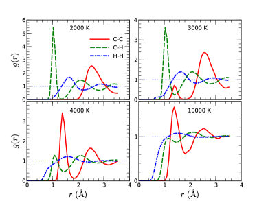
Figure 9: Pair correlation functions, $g(r)$, between different nuclei as a function of temperature at a density of 2.0 g cm^-3. The intramolecular C-H and H-H peaks at 1.05 and 1.7 Å disappear as CH₄ molecules dissociate with increasing temperature, while the intensity of the C-C peak at 1.4 Å rises with increased polymerization and then drops again as a plasma state is reached at 10 000 K.

The structure of the fluid was further investigated by examination of pair correlation functions as shown in Fig. 9. All pair correlation functions were computed at the density 2.0 g cm^-3. At 2000 K, methane molecules clearly dominate the system. The large peak at 1.05 Å corresponds to the C–H bond of methane. This peak is followed by a minimum close to zero, which is indicative of stable molecules. When the temperature is raised to 3000 K, a new C–C peak begins to emerge at 1.4 Å, corresponding to the carbon bonds in longer hydrocarbon chains. A corresponding decrease in the C–H peak, and the appearance of a H–H peak of molecular hydrogen, is also seen. At 4000 K, these processes become more apparent, as the C–C peak at 1.4 Å intensified and the C–H peak diminished. The flattening of the H–H curve is a consequence of the dissociation of the methane molecules. Lastly, at 10 000 K the C–C peak, while reduced, is still evident. However, at this temperature all molecules are very short lived and unstable, and the broadening of C–H and H–H peaks illustrate this fact.

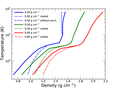
Figure 10: Subset of Hugoniot curves from Fig. 1 for three initial densities, $\rho_{0}$, specified in the legend. The dashed lines correspond to polymeric samples that have been cooled from simulations at 4000 K. The dash-dotted line refers to simulations without contributions from excited electronic states.

We predicted the shock Hugoniot curves for the polymeric state by cooling the simulations from 4000 to 300 K at six different densities from 0.8 to 2.0 g cm^-3. Starting from the geometries and velocities at 4000 K, we lowered the temperature in intervals of 1000 K by rescaling the velocities and performing MD simulations for 2 ps at each step. The structure of hydrocarbons, that were initially present, change very little during the cooling simulations because the temperature dropped below the activation barrier for such reactions. As expected, all simulations eventually froze. For $\rho=1.2\,$g cm^-3, it attained a composition of C₉H₂₀ + C₆H₁₄ + 2C₂H₆ + 8CH₄ + 15H₂. These finding resemble results of the shock experiment by Hirai et al. hirai , who observed that the hydrocarbons produced did not revert back to methane when the samples were cooled.

Figure 10 shows the Hugoniot curves for a cooled simulation corresponding to three different initial densities. At 4000 K, they converge to our original Hugoniot curves but deviations become increasingly pronounced with decreasing temperature, culminating in a density increase of, respectively, 0.23 (31%), 0.21 (24%), and 0.17 g cm^-3 (24%) for the initial densities of $\rho_{0}$ = 0.4, 0.5, and 0.6 g cm^-3 at 300 K. Because we kept the initial parameters, $E_{0}$ and $V_{0}$, of methane in Eq. 1, the deviations between the original and the polymeric Hugoniot curves persist in the limit of zero temperature. We predict the findings of a future shock experiment on methane to fall in between both sets of curves. For low shock velocities, one would expect the results to track our original Hugoniot curves for stable molecules. For higher shock speeds, the sample in the experiment may convert to a polymeric state at lower temperatures than we see in our simulations. In this case, we predict a significant increase in density to occur that shifts the measured Hugoniot curve from the original towards the polymeric Hugoniot curve. Figure 3 suggests that this may be accompanied by a drop in pressure and a modest change in optical properties.

In shock experiments, one may observe the transformation into a polymeric state at lower temperatures than we predict with our simulations because experiments last for nanoseconds and samples are much larger. However, also experiments may also not reach chemical equilibrium at lower temperatures because the activitation energies for different chemical reactions may be higher than the available kinetic energy that could trigger such reaction.

The fact that the molecular and the polymeric Hugoniot curve diverge below 4000 K in Fig. 10 also has implications for decaying shock experiments eggert10 . This new experimental technique allows one to map out a whole segment of the Hugoniot curve with a single shock wave experiment. At the beginning of the shock propagation, the material in compressed to a state of high pressure and temperature on the Hugoniot curve. As the shock wave continues to propagate, the particle velocity is gradually reduced and new material is compressed to a lower pressure and temperature. The shock velocity is continuously monitored with an interferometer so that a whole segment of Hugoniot curve can be measured in one shock experiment. If a decaying shock acrosses the polymeric regime of methane, we predict the following to occur. As the shock enters the polymeric regime, new material at the shock front would still be compressed as in a usual shock experiments and may yield a state on the molecular or on the polymeric Hugoniot, as we discussed. However, as material behind the shock front expands from a high-temperature state, it will change from a plasma into the polymeric state rather than converting back to molecular methane, as we have observed in our cooled simulations in Fig. 3. This may lead to a structured shock wave with various parts in different thermodynamic states. So the polymerization of methane may provide a mechanism for introducing a shock velocity reversal that were observed in  Spaulding2012 and discussed in Militzer2012 .

Finally, we investigated the effects that thermal electronic excitation have on the shape of the Hugoniot curves. While electronic excitations were included in all simulations discussed so far, we performed some DFT-MD simulations where the electrons were kept in the ground state. This resulted into drastic reductions of the computed pressures and internal energies but both effects nearly cancelled Mi06 when the Hugoniot curve was calculated. So Figure 10 shows only a modest shift towards lower densities for temperatures over 10 000 K.

III Conclusions

We identified and characterized molecular, polymeric, and plasma states in the phase diagram of methane by analyzing the of the liquid in DFT-MD simulations that we performed in a temperature-density range from 300 to 75 000 K and 0.8 to 2.5 g cm^-3. We presented shock Hugoniot curves for initial densities from 0.35 to 0.70 g cm^-3. We predict a drastic increase in density along the Hugoniot curves as the sample transforms into a polymeric state. This transformation is accompanied by an increase in reflectivity and electrical conductivity because the polymeric state is metallic.

This state is also prone to dehydrogenation reactions, which has implications for the interiors of Uranus and Neptune. These planets’ isentropes intersect the temperature-pressure conditions of the polymeric regime and thus molecular hydrogen may be released from ice layers of both planets. This could lead to more compact cores in Uranus and Neptune, in contrast to recent predictions of core erosion for Jupiter and Saturn WilsonMilitzer2012 ; WilsonMilitzer2012b .

We also argued that the dehydrogenation reactions prevent methane from assuming a superionic state at high pressure and temperature that was predicted for water and ammonia cavazzoni . However more theoretical and experimental work on mixture of planetary ices will be required to provide much-needed constraints for the interiors of ice giant planets NewHelledPaper .

Acknowledgements: This work was supported by NASA and NSF. Computational resources were supplied in part by NCCS and TAC.

The following table is to be published as online supplementary information

$T$ (K)	$P$ (GPa)	$E$ (eV/CH4)
	$\rho$= 0.600 g cm-3
300	1.957(10)	$-$0.173451(13)
	$\rho$= 0.800 g cm-3
300	6.984(18)	$-$0.172014(10)
1000	8.68(4)	$-$0.16580(5)
2000	10.47(3)	$-$0.15674(3)
3000	12.35(9)	$-$0.14831(8)
4000	14.37(11)	$-$0.1354(3)
	$\rho$= 1.000 g cm-3
300	15.73(4)	$-$0.169205(11)
1000	17.93(4)	$-$0.16274(2)
2000	20.84(11)	$-$0.15374(6)
3000	24.02(10)	$-$0.14456(8)
4000	25.00(13)	$-$0.1321(2)
	$\rho$= 1.201 g cm-3
300	28.309(19)	$-$0.165345(9)
1000	32.42(5)	$-$0.15855(2)
2000	36.57(12)	$-$0.14920(4)
3000	40.05(11)	$-$0.13961(8)
4000	40.4(3)	$-$0.1237(4)
5000	40.41(14)	$-$0.1067(2)
6000	43.65(16)	$-$0.0960(2)
7000	47.0(3)	$-$0.08730(11)
10000	59.76(9)	$-$0.06481(12)
20000	107.47(20)	0.00630(11)
30000	158.44(16)	0.08227(10)
40000	212.5(3)	0.16452(12)
75000	417.0(3)	0.49150(13)
	$\rho$= 1.353 g cm-3
2000	52.81(10)	$-$0.14496(5)
	$\rho$= 1.498 g cm-3
300	59.48(3)	$-$0.157294(10)
1000	64.55(8)	$-$0.15038(3)
2000	70.97(16)	$-$0.14057(5)
3000	75.87(17)	$-$0.13066(6)
4000	71.09(15)	$-$0.1126(3)
5000	72.76(19)	$-$0.0984(2)
6000	77.7(4)	$-$0.08951(14)
7000	83.7(2)	$-$0.0815(2)
10000	100.79(14)	$-$0.05941(8)
20000	162.79(20)	0.01036(11)
30000	229.0(6)	0.0870(11)
40000	292.7(1.7)	0.1658(10)
75000	550.8(4)	0.48502(13)
	$\rho$= 1.600 g cm-3
2000	85.39(16)	$-$0.13698(5)
3000	90.95(14)	$-$0.12687(11)
4000	84.02(19)	$-$0.1086(2)
5000	87.5(2)	$-$0.09565(18)
10000	118.6(2)	$-$0.05693(9)
20000	185.2(4)	0.0129(4)
30000	254.2(4)	0.08663(10)
40000	326.4(3)	0.16661(18)
75000	599.8(5)	0.4841(2)

$T$ (K)	$P$ (GPa)	$E$ (eV/CH4)
	$\rho$= 1.775 g cm-3
2000	115.04(19)	$-$0.13039(4)
3000	120.6(3)	$-$0.11986(11)
4000	110.0(4)	$-$0.1018(2)
5000	116.36(13)	$-$0.09025(13)
10000	151.85(18)	$-$0.05220(9)
20000	227.5(3)	0.01736(12)
30000	304.6(5)	0.0917(6)
40000	383.3(9)	0.1700(2)
75000	687.1(8)	0.4836(3)
	$\rho$= 2.010 g cm-3
2000	161.77(17)	$-$0.12039(6)
3000	154.4(4)	$-$0.10612(16)
4000	155.5(2)	$-$0.09276(11)
5000	162.68(13)	$-$0.08206(10)
10000	205.9(3)	$-$0.04411(10)
20000	292.0(4)	0.0250(2)
30000	380.4(3)	0.09839(18)
40000	469.6(6)	0.1763(3)
75000	811.9(6)	0.4857(2)
	$\rho$= 2.129 g cm-3
10000	236.22(19)	$-$0.03969(9)
	$\rho$= 2.257 g cm-3
5000	222.7(3)	$-$0.07214(11)
10000	272.8(5)	$-$0.03438(14)
20000	369.9(4)	0.03459(13)
30000	468.9(6)	0.10728(18)
40000	569.2(6)	0.1843(2)
75000	954.7(6)	0.49147(16)
	$\rho$= 2.376 g cm-3
10000	308.3(4)	$-$0.02945(12)
	$\rho$= 2.502 g cm-3
5000	292.4(5)	$-$0.06108(13)
10000	349.7(5)	$-$0.02343(16)
20000	457.5(2)	0.04569(10)
30000	566.9(9)	0.1180(2)
40000	679.6(5)	0.19499(14)
75000	883.4(7)	0.32519(17)

Table 1: Pressure and internal energy from our DFT-MD simulations at various densities and temperatures. The 1 $\sigma$ error bars are given in brackets.

References

- (1) W. B. Hubbard, Science 214, 145 (1981).
- (2) H. F. Wilson and B. Militzer. Astrophys. J, 745:54, 2012.
- (3) H. F. Wilson and B. Militzer. Phys. Rev. Lett., 108:111101, 2012.
- (4) W. J. Borucki et al., The Astrophysical Journal, 726 19 (2011).
- (5) D. G. Hicks, T. R. Boehly, J. H. Eggert, J. E. Miller, P. M. Celliers, and G. W. Collins. Phys. Rev. Lett., 97:025502, 2006.
- (6) M. D. Knudson and M. P. Desjarlais. Phys. Rev. Lett., 103:225501, 2009.
- (7) K. K. M. Lee et al. J. Chem Phys., 125:014701, 2006.
- (8) B. Militzer and W. B. Hubbard. AIP Conf. Proc., 955:1395, 2007.
- (9) R. Jeanloz, P. M. Celliers, G. W. Collins, J. H. Eggert, K. K. M. Lee, R. S. McWilliams, S. Brygoo, and P. Loubeyre. Proc. Nat. Acad. Sci., 107:9172, 2007.
- (10) D. K. Spaulding et al. Phys. Rev. Lett., 108:065701, 2012.
- (11) B. Militzer, ”Ab Initio Investigation of a Possible Liquid-Liquid Phase Transition in MgSiO3 at Megabar Pressures”, submitted to the Journal of High Energy Density Physics (2012).
- (12) B. Militzer and D. M. Ceperley. Phys. Rev. Lett., 85:1890, 2000.
- (13) B. Militzer, D. M. Ceperley, J. D. Kress, J. D. Johnson, L. A. Collins, and S. Mazevet. Phys. Rev. Lett., 87:275502, 2001.
- (14) B. Militzer. Phys. Rev. B, 79:155105, 2009.
- (15) B. Militzer. Phys. Rev. Lett., 97:175501, 2006.
- (16) B. Militzer, F. Gygi, and G. Galli. Phys. Rev. Lett., 91:265503, 2003.
- (17) L. R. Benedetti, J. H. Nguyen, W. A. Caldwell, H. Liu, M. Kruger and R. Jeanloz, Science 284 100 (1999)
- (18) H. Hirai, K. Konagai, T. Kawamura, Y. Yamamoto and T. Yagi, Phys. Earth. Planet. Inter. 174 242 (1999).
- (19) W. J. Nellis, D. C. Hamilton and A. C. Mitchell, J. Chem. Phys. 115 1015 (2001).
- (20) H. B. Radousky, A. C. Mitchell and W. J. Nellis, J. Chem. Phys. 93, 8235 (1990).
- (21) F. Ancilotto, G. L. Chiarotti, S. Scandolo, E. Tosatti, Science 275, 1288 (1997).
- (22) L. Spanu, D. Donadio, D. Hohl, E. Schwegler and G. Galli, Proc. Nat. Acad. Sci. 108 6843 (2011).
- (23) G. Gao, A. R. Oganov, Y. Ma, H. Wang, P. Li, Y. Li, T. Iitaka, and G. Zou, J. Chem. Phys 133 144508 (2010).
- (24) N. Goldman, E. J. Reed and L. E. Fried, J. Chem. Phys. 131, 204103 (2009).
- (25) Y. B. Zeldovich and Y. P. Raizer, Physics of Shock Waves and High-Temperature Hydrodynamic Phenomena, Academic Press, New York (1966).
- (26) G. Kresse and J. Furthmüller, Phys. Rev. B 54, 11169 (1996).
- (27) P. E. Blochl, Phys. Rev. B 50, 17953 (1994).
- (28) J. P. Perdew, K. Burke, and M. Ernzerhof, Phys. Rev. Lett. 77, 3865 (1996).
- (29) R. Redmer, T. R. Mattsson, N. Nettelmann, and M. French Icarus 211 798 (2011).
- (30) N. D. Mermin. Phys. Rev., 137:A1441, 1965.
- (31) L. Stixrude and R. Jeanloz. Proc. Nat. Ac. Sci., 105:11071, 2008.
- (32) P. M. Celliers, P. Loubeyre, J. H. Eggert, S. Brygoo, R. S. McWilliams, D. G. Hicks, T. R. Boehly, R. Jeanloz, and G. W. Collins1. Phys. Rev. Lett., 104:184503, 2010.
- (33) C. Cavazzoni, G. L. Chiarotti, S. Scandolo, E. Tosatti, M. Bernasconi, and M. Parrinello. Nature, 283:44, 1999.
- (34) B. Militzer, W. H. Hubbard, J. Vorberger, I. Tamblyn and S. A. Bonev Astrophys. J. Lett., 688:L45, 2008.
- (35) M. A. Morales, C. Pierleoni, E. Schwegler and D. M. Ceperley. Proc. Nat. Acad. Sci. 107:12799, 2010.
- (36) J. H. Eggert, D. G. Hicks, P. M. Celliers, D. K. Bradley, R. S. McWilliams, R. Jeanloz, J. E. Miller, T. R. Boehly, and G. W. Collins. Nature Phys., 6:40, 2010.
- (37) R. Helled, J. D. Anderson, M. Podolak and G. Schubert, Astrophys. J. 726:15, 2011.