Expectation Propagation in
Gaussian Process Dynamical Systems:
Extended Version

Abstract

Rich and complex time-series data, such as those generated from engineering systems, financial markets, videos or neural recordings, are now a common feature of modern data analysis. Explaining the phenomena underlying these diverse data sets requires flexible and accurate models. In this paper, we promote Gaussian process dynamical systems (GPDS) as a rich model class that is appropriate for such analysis. In particular, we present a message passing algorithm for approximate inference in GPDSs based on expectation propagation. By posing inference as a general message passing problem, we iterate forward-backward smoothing. Thus, we obtain more accurate posterior distributions over latent structures, resulting in improved predictive performance compared to state-of-the-art GPDS smoothers, which are special cases of our general message passing algorithm. Hence, we provide a unifying approach within which to contextualize message passing in GPDSs.

1 Introduction

The Kalman filter and its extensions [1], such as the extended and unscented Kalman filters [8], are principled statistical models that have been widely used for some of the most challenging and mission-critical applications in automatic control, robotics, machine learning, and economics. Indeed, wherever complex time-series are found, Kalman filters have been successfully applied for Bayesian state estimation. However, in practice, time series often have an unknown dynamical structure, and they are high dimensional and noisy, violating many of the assumptions made in established approaches for state estimation. In this paper, we look beyond traditional linear dynamical systems and advance the state-of the-art in state estimation by developing novel inference algorithms for the class of nonlinear Gaussian process dynamical systems (GPDS).

GPDSs are non-parametric generalizations of state-space models that allow for inference in time series, using Gaussian process (GP) probability distributions over nonlinear transition and measurement dynamics. GPDSs are thus able to capture complex dynamical structure with few assumptions, making them of broad interest. This interest has sparked the development of general approaches for filtering and smoothing in GPDSs, such as  [9, 4, 6]. In this paper, we further develop inference algorithms for GPDSs and make the following contributions: (1) We develop an iterative local message passing framework for GPDSs based on Expectation Propagation (EP) [12, 11], which allows for refinement of the posterior distribution and, hence, improved inference. (2) We show that the general message-passing framework recovers the EP updates for existing dynamical systems as a special case and expose the implicit modeling assumptions made in these models. We show that EP in GPDSs encapsulates all GPDS forward-backward smoothers [6] as a special case and transforms them into iterative algorithms yielding more accurate inference.

2 Gaussian Process Dynamical Systems

Gaussian process dynamical systems are a general class of discrete-time state-space models with

$$\boldsymbol{x}_{t}=h(\boldsymbol{x}_{t-1})+\boldsymbol{w}_{t}\,,\quad\boldsymbol{w}_{t}\sim\mathcal{N}(\boldsymbol{0},\boldsymbol{Q})\,,\quad h\sim\mathcal{GP}_{h}\,,$$ (1)

$$\boldsymbol{z}_{t}=g(\boldsymbol{x}_{t})+\boldsymbol{v}_{t}\,,\quad\boldsymbol{v}_{t}\sim\mathcal{N}(\boldsymbol{0},\boldsymbol{R})\,,\quad g\sim\mathcal{GP}_{g}\,,$$ (2)

where $t=1,\dotsc,T$. Here, $\boldsymbol{x}\in\mathds{R}^{D}$ is a latent state that evolves over time, and $\boldsymbol{z}\in\mathds{R}^{E}$, $E\geq D$, are measurements. We assume i.i.d. additive Gaussian system noise $\boldsymbol{w}$ and measurement noise $\boldsymbol{v}$. The central feature of this model class is that both the measurement function $g$ and the transition function $h$ are not explicitly known or parametrically specified, but instead described by probability distributions over these functions. The function distributions are non-parametric Gaussian processes (GPs), and we write $h\sim\mathcal{GP}_{h}$ and $g\sim\mathcal{GP}_{g}$, respectively.

A GP is a probability distribution $p(f)$ over functions $f$ that is specified by a mean function $\mu_{f}$ and a covariance function $k_{f}$ [16]. Consider a set of training inputs $\boldsymbol{X}=[\boldsymbol{x}_{1},\dotsc,\boldsymbol{x}_{n}]^{\top}$ and corresponding training targets $\boldsymbol{y}=[y_{1},\dotsc y_{n}]^{\top}$, $y_{i}=f(\boldsymbol{x}_{i})+w$, $w\sim\mathcal{N}(0,\sigma_{w}^{2})$. The posterior predictive distribution at a test input $\boldsymbol{x}_{*}$ is Gaussian distributed $\mathcal{N}(y_{*}\,|\,\mu_{f}(\boldsymbol{x}_{*}),\sigma_{f}^{2}(\boldsymbol{x}_{*}))$ with mean $\mu_{f}(\boldsymbol{x}_{*})=\boldsymbol{k}_{*}^{\top}\boldsymbol{K}^{-1}\boldsymbol{y}$ and variance $\sigma_{f}^{2}(\boldsymbol{x}_{*})=k_{**}-\boldsymbol{k}_{*}^{\top}\boldsymbol{K}^{-1}\boldsymbol{k}_{*}$, where $\boldsymbol{k}_{*}=k_{f}(\boldsymbol{X},\boldsymbol{x}_{*})$, $k_{**}=k_{f}(\boldsymbol{x}_{*},\boldsymbol{x}_{*})$, and $\boldsymbol{K}$ is the kernel matrix.

Since the GP is a non-parametric model, its use in GPDSs is desirable since it results in fewer restrictive model assumptions, compared to dynamical systems based on parametric function approximators for the transition and measurement functions (1)–(2). In this paper, we assume that the GP models are trained, i.e., the training inputs and corresponding targets as well as the GP hyperparameters are known. For both $\mathcal{GP}_{h}$ and $\mathcal{GP}_{g}$ in the GPDS, we used zero prior mean functions. As covariance functions $k_{h}$ and $k_{g}$ we use squared- exponential covariance functions with automatic relevance determination plus a noise covariance function to account for the noise in (1)–(2).

Existing work for learning GPDSs includes the Gaussian process dynamical model (GPDM) [21], which tackles the challenging task of analyzing human motion in (high-dimensional) video sequences. More recently, variational [3] and EM-based [20] approaches for learning GPDS were proposed. Exact Bayesian inference, i.e., filtering and smoothing, in GPDSs is analytically intractable because of the dependency of the states and measurements on previous states through the nonlinearity of the GP. We thus make use of approximations to infer the posterior distributions $p(\boldsymbol{x}_{t}|\boldsymbol{Z})$ over latent states $\boldsymbol{x}_{t}$, $t=1,\dotsc,T$, given a set of observations $\boldsymbol{Z}=\boldsymbol{z}_{1:T}$. Existing approximate inference approaches for filtering and forward-backward smoothing are based on either linearization, particle representations, or moment matching as approximation strategies [9, 4, 6].

A principled incorporation of the posterior GP model uncertainty into inference in GPDSs is necessary, but introduces additional uncertainty. In tracking problems where the location of an object is not directly observed, this additional source of uncertainty can eventually lead to losing track of the latent state. In this paper, we address this problem and propose approximate message passing based on EP for more accurate inference. We will show that forward-backward smoothing in GPDSs [6] benefits from the iterative refinement scheme of EP, leading to more accurate posterior distributions over the latent state and, hence, to more informative predictions and improved decision making.

3 Expectation Propagation in GPDS

Expectation Propagation [11, 12] is a widely-used deterministic algorithm for approximate Bayesian inference that has been shown to be highly accurate in many problems, including sparse regression models [18], GP classification [10], and inference in dynamical systems [14, 7, 19]. EP is derived using a factor-graph, in which the distribution over the latent state $p(\boldsymbol{x}_{t}|\boldsymbol{Z})$ is represented as the product of factors $f_{i}(\boldsymbol{x}_{t})$, i.e., $p(\boldsymbol{x}_{t}|\boldsymbol{Z})=\prod_{i}f_{i}(\boldsymbol{x}_{t})$. EP then specifies an iterative message passing algorithm in which $p(\boldsymbol{x}_{t}|\boldsymbol{Z})$ is approximated by a distribution $q(\boldsymbol{x}_{t})=\prod_{i}q_{i}(\boldsymbol{x}_{t})$, using approximate messages $q_{i}(\boldsymbol{x}_{t})$. In EP, $q$ and the messages $q_{i}$ are members of the exponential family, and $q$ is determined such that the the KL-divergence KL$(p||q)$ is minimized. EP is provably robust for log-concave messages [18] and invariant under invertible variable transformations [17]. In practice, EP has been shown to be more accurate than competing approximate inference methods [10, 18].

Figure 1: Factor graph (left) and fully factored graph (right) of a general dynamical system.

In the context of the dynamical system (1)–(2), we consider factor graphs of the form of Fig. 1 with three types of messages: forward, backward, and measurement messages, denoted by the symbols ${\vartriangleright},{\vartriangleleft},{\vartriangle}$, respectively. For EP inference, we assume a fully-factored graph, using which we compute the marginal posterior distributions $p(\boldsymbol{x}_{1}|\boldsymbol{Z}),\dotsc,p(\boldsymbol{x}_{T}|\boldsymbol{Z})$, rather than the full joint distribution $p(\boldsymbol{X}|\boldsymbol{Z})=p(\boldsymbol{x}_{1},\dotsc,\boldsymbol{x}_{T}|\boldsymbol{Z})$. Both the states $\boldsymbol{x}_{t}$ and measurements $\boldsymbol{z}_{t}$ are continuous variables and the messages $q_{i}$ are unnormalized Gaussians, i.e., $q_{i}(\boldsymbol{x}_{t})=s_{i}\mathcal{N}(\boldsymbol{x}_{t}\,|\,\boldsymbol{\mu}_{i},\boldsymbol{\Sigma}_{i})$

3.1 Implicit Linearizations Require Explicit Consideration

Algorithm 1 Gaussian EP for Dynamical Systems

1:Init: Set all factors $q_{i}$ to $\mathcal{N}(\boldsymbol{0},\infty\boldsymbol{I})$; Set $q(\boldsymbol{x}_{1})=p(\boldsymbol{x}_{1})$ and marginals $q(\boldsymbol{x}_{t\neq 1})=\mathcal{N}(\boldsymbol{0},10^{10}\boldsymbol{I})$

2:repeat

3:     for $t=1$ to $T$ do

4:         for all factors $q_{i}(\boldsymbol{x}_{t})$, where $i={\vartriangleright},{\vartriangle},{\vartriangleleft}$ do

5:              Compute cavity distribution $q^{\setminus i}(\boldsymbol{x}_{t})=q(\boldsymbol{x}_{t})/q_{i}(\boldsymbol{x}_{t})=\mathcal{N}(\boldsymbol{x}_{t}\,|\,\boldsymbol{\mu}^{\setminus i},\boldsymbol{\Sigma}^{\setminus i})$ with

$$\boldsymbol{\Sigma}^{\setminus i} =(\boldsymbol{\Sigma}_{t}^{-1}-\boldsymbol{\Sigma}_{i}^{-1})^{-1}\,,\qquad\boldsymbol{\mu}^{\setminus i}=\boldsymbol{\Sigma}^{\setminus i}(\boldsymbol{\Sigma}_{t}^{-1}\boldsymbol{\mu}_{t}-\boldsymbol{\Sigma}_{i}^{-1}\boldsymbol{\mu}_{i})$$ (3)

6:              Determine moments of $f_{i}(\boldsymbol{x}_{t})q^{\setminus i}(\boldsymbol{x}_{t})$, e.g., via the derivatives of

$$\log Z_{i}(\boldsymbol{\mu}^{\setminus i},\boldsymbol{\Sigma}^{\setminus i}) =\log\smallint f_{i}(\boldsymbol{x}_{t})q^{\setminus i}(\boldsymbol{x}_{t})\mathrm{d}\boldsymbol{x}_{t}$$ (4)

7:              Update the posterior $q(\boldsymbol{x}_{t})\propto\mathcal{N}(\boldsymbol{x}_{t}\,|\,\boldsymbol{\mu}_{t},\boldsymbol{\Sigma}_{t})$ and the approximate factor $q_{i}(\boldsymbol{x}_{t})$:

$$\boldsymbol{\mu}_{t} =\boldsymbol{\mu}^{\setminus i}+\boldsymbol{\Sigma}^{\setminus i}\boldsymbol{\nabla}_{m}^{\top}\,,\qquad\boldsymbol{\Sigma}_{t}=\boldsymbol{\Sigma}^{\setminus i}-\boldsymbol{\Sigma}^{\setminus i}(\boldsymbol{\nabla}_{m}^{\top}\boldsymbol{\nabla}_{m}-2\boldsymbol{\nabla}_{s})\boldsymbol{\Sigma}^{\setminus i}$$ (5)

$$\boldsymbol{\nabla}_{m} \coloneqq\mathrm{d}\log Z_{i}/\mathrm{d}\boldsymbol{\mu}^{\setminus i}\,,\qquad\boldsymbol{\nabla}_{s}\coloneqq\mathrm{d}\log Z_{i}/\mathrm{d}{\boldsymbol{\Sigma}^{\setminus i}}$$ (6)

$$q_{i}(\boldsymbol{x}_{t}) =q(\boldsymbol{x}_{t})/q^{\setminus i}(\boldsymbol{x}_{t})$$ (7)

8:         end for

9:     end for

10:until Convergence or maximum number of iterations exceeded

Alg. 1 describes the main steps of Gaussian EP for dynamical systems. For each node $\boldsymbol{x}_{t}$ in the fully-factored factor graph in Fig. 1, EP computes three messages: a forward, backward, and measurement message, denoted by $q_{{\vartriangleright}}(\boldsymbol{x}_{t})$, $q_{{\vartriangleleft}}(\boldsymbol{x}_{t})$, and $q_{{\vartriangle}}(\boldsymbol{x}_{t})$, respectively. The EP algorithm updates the marginal $q(\boldsymbol{x}_{t})$ and the messages $q_{i}(\boldsymbol{x}_{t})$ in three steps. First, the cavity distribution $q^{\setminus i}(\boldsymbol{x}_{t})$ is computed (step 5 in Alg. 1) by removing $q_{i}(\boldsymbol{x}_{t})$ from the marginal $q(\boldsymbol{x}_{t})$. Second, in the projection step, the moments of $f_{i}(\boldsymbol{x}_{t})q^{\setminus i}(\boldsymbol{x}_{t})$ are computed (step 6), where $f_{i}$ is the true factor. In the exponential family, the required moments can be computed using the derivatives of the log-partition function (normalizing constant) $\log Z_{i}$ of $f_{i}(\boldsymbol{x}_{t})q^{\setminus i}(\boldsymbol{x}_{t})$ [11, 12, 13]. Third, the moments of the marginal $q(\boldsymbol{x}_{t})$ are set to the moments of $f_{i}(\boldsymbol{x}_{t})q^{\setminus i}(\boldsymbol{x}_{t})$, and the message $q_{i}(\boldsymbol{x}_{t})$ is updated (step 7). We apply this procedure repeatedly to all latent states $\boldsymbol{x}_{t}$, $t=1,\dotsc,T$, until convergence.

EP does not directly fit a Gaussian approximation $q_{i}$ to the non-Gaussian factor $f_{i}$. Instead, EP determines the moments of $q_{i}$ in the context of the cavity distribution such that $q_{i}=\mathrm{proj}[f_{i}q^{\setminus i}]/q^{\setminus i}$, where $\mathrm{proj}[\cdot]$ is the projection operator, returning the moments of its argument.

To update the posterior $q(\boldsymbol{x}_{t})$ and the messages $q_{i}(\boldsymbol{x}_{t})$, EP computes the log-partition function $\log Z_{i}$ in (4) to complete the projection step. However, for nonlinear transition and measurement models in (1)–(2), computing $Z_{i}$ involves solving integrals of the form

$$p(\boldsymbol{a})=\int p(\boldsymbol{a}|\boldsymbol{x}_{t})p(\boldsymbol{x}_{t})\mathrm{d}\boldsymbol{x}_{t}=\int\mathcal{N}(\boldsymbol{a}\,|\,\boldsymbol{m}(\boldsymbol{x}_{t}),\boldsymbol{S}(\boldsymbol{x}_{t}))\mathcal{N}(\boldsymbol{x}_{t}\,|\,\boldsymbol{b},\boldsymbol{B})\mathrm{d}\boldsymbol{x}_{t}\,,$$ (8)

where $\boldsymbol{a}=\boldsymbol{z}_{t}$ for the measurement message, or $\boldsymbol{a}=\boldsymbol{x}_{t+1}$ for the forward and backward messages. In nonlinear dynamical systems $\boldsymbol{m}(\boldsymbol{x}_{t})$ is a nonlinear measurement or transition function. In GPDSs, $\boldsymbol{m}(\boldsymbol{x}_{t})$ and $\boldsymbol{S}(\boldsymbol{x}_{t})$ are the corresponding predictive GP means and covariances, respectively, which are nonlinearly related to $\boldsymbol{x}_{t}$. Because of the nonlinear dependencies between $\boldsymbol{a}$ and $\boldsymbol{x}_{t}$, solving (8) is analytically intractable. We propose to approximate $p(\boldsymbol{a})$ by a Gaussian distribution $\mathcal{N}(\boldsymbol{a}\,|\,\tilde{\boldsymbol{\mu}},\tilde{\boldsymbol{\Sigma}})$. This Gaussian approximation is only correct for a linear relationship $\boldsymbol{a}=\boldsymbol{J}\boldsymbol{x}_{t}$, where $\boldsymbol{J}$ is independent of $\boldsymbol{x}_{t}$. Hence, the Gaussian approximation is an implicit linearization of the functional relationship between $\boldsymbol{a}$ and $\boldsymbol{x}_{t}$, effectively linearizing either the transition or the measurement models.

When computing EP updates using the derivatives $\boldsymbol{\nabla}_{m}$ and $\boldsymbol{\nabla}_{s}$ according to (5) it is crucial to explicitly account for the implicit linearization assumption in the derivatives—otherwise, the EP updates are inconsistent. For example, in the measurement and the backward message, we directly approximate the partition functions $Z_{i}$, $i\in\{{\vartriangle},{\vartriangleleft}\}$ by Gaussians $\tilde{Z}_{i}(\boldsymbol{a})=\mathcal{N}(\tilde{\boldsymbol{\mu}}^{i},\tilde{\boldsymbol{\Sigma}}^{i})$. The consistent derivatives $\mathrm{d}(\log\tilde{Z}_{i})/\mathrm{d}\boldsymbol{\mu}^{\setminus i}$ and $\mathrm{d}(\log\tilde{Z}_{i})/\mathrm{d}\boldsymbol{\Sigma}^{\setminus i}$ of $\tilde{Z}_{i}$ with respect to the mean and covariance of the cavity distribution $q$ are obtained by applying the chain rule, such that

$$\boldsymbol{\nabla}_{m} =\tfrac{\mathrm{d}\log\tilde{Z}_{i}}{\mathrm{d}\boldsymbol{\mu}^{\setminus i}}=\tfrac{\partial\log\tilde{Z}_{i}}{\partial\tilde{\boldsymbol{\mu}}^{i}}\tfrac{\partial\tilde{\boldsymbol{\mu}}^{i}}{\partial\boldsymbol{\mu}^{\setminus i}}=(\boldsymbol{a}-\tilde{\boldsymbol{\mu}}^{i})^{\top}(\tilde{\boldsymbol{\Sigma}}^{i})^{-1}\boldsymbol{J}^{\top}\in\mathds{R}^{1\times D}\,,$$ (9)

$$\boldsymbol{\nabla}_{s} =\tfrac{\mathrm{d}\log\tilde{Z}_{i}}{\mathrm{d}\boldsymbol{\Sigma}^{\setminus i}}=\tfrac{\partial\log\tilde{Z}_{i}}{\partial\tilde{\boldsymbol{\Sigma}}^{i}}\tfrac{\partial\tilde{\boldsymbol{\Sigma}}^{i}}{\partial\boldsymbol{\Sigma}^{\setminus i}}=\tfrac{1}{2}\left(\tfrac{\partial\log\tilde{Z}_{i}}{\partial(\tilde{\boldsymbol{\mu}}^{i})^{\top}}\tfrac{\partial\log\tilde{Z}_{i}}{\partial\tilde{\boldsymbol{\mu}}^{i}}-(\tilde{\boldsymbol{\Sigma}}^{i})^{-1}\right)\tfrac{\partial\tilde{\boldsymbol{\Sigma}}^{i}}{\partial\boldsymbol{\Sigma}^{\setminus i}}\in\mathds{R}^{D\times D}\,,$$ (10)

$$\tfrac{\partial\tilde{\boldsymbol{\mu}}^{i}}{\partial\boldsymbol{\mu}^{\setminus i}} =\boldsymbol{J}^{\top}\in\mathds{R}^{E\times D}\,,\quad\tfrac{\partial\tilde{\boldsymbol{\Sigma}}^{i}}{\partial\boldsymbol{\Sigma}^{\setminus i}}=\boldsymbol{J}\mathds{I}_{4}\boldsymbol{J}^{\top}\in\mathds{R}^{E\times E\times D\times D}\,,$$ (11)

where $\mathds{I}_{4}\in\mathds{R}^{D\times D\times D\times D}$ is an identity tensor. Note that with the implicit linear model $\boldsymbol{a}=\boldsymbol{J}\boldsymbol{x}_{t}$, the derivatives $\partial\tilde{\boldsymbol{\mu}}^{i}/\partial\boldsymbol{\Sigma}^{\setminus i}$ and $\partial\tilde{\boldsymbol{\Sigma}}^{i}/\partial\boldsymbol{\mu}^{\setminus i}$ vanish. Although we approximate $Z_{i}$ by a Gaussian $\tilde{Z}_{i}$, we are still free to choose a method of computing its mean $\tilde{\boldsymbol{\mu}}^{i}$ and covariance matrix $\tilde{\boldsymbol{\Sigma}}^{i}$, which also influences the computation of $\boldsymbol{J}=\partial(\tilde{\boldsymbol{\mu}}^{i})/\partial\boldsymbol{\mu}^{\setminus i}$. However, even if $\tilde{\boldsymbol{\mu}}^{i}$ and $\tilde{\boldsymbol{\Sigma}}^{i}$ are general functions of $\boldsymbol{\mu}^{\setminus i}$ and $\boldsymbol{\Sigma}^{\setminus i}$, the derivatives $\partial\tilde{\boldsymbol{\mu}}^{i}/\partial\boldsymbol{\mu}^{\setminus i}$ and $\partial\tilde{\boldsymbol{\Sigma}}^{i}/\partial\boldsymbol{\Sigma}^{\setminus i}$ must equal the corresponding partial derivatives in (11), and $\partial\tilde{\boldsymbol{\mu}}^{i}/\partial\boldsymbol{\Sigma}^{\setminus i}$ and $\partial\tilde{\boldsymbol{\Sigma}}^{i}/\partial\boldsymbol{\mu}^{\setminus i}$ must be set to $\boldsymbol{0}$. Hence, the implicit linearization expressed by the Gaussian approximation $\tilde{Z}_{i}$ must be explicitly taken into account in the derivatives to guarantee consistent EP updates.

3.2 Messages in Gaussian Process Dynamical Systems

We now describe each the messages needed for inference in GPDSs, and outline the approximations required to compute the partition function in (4). Updating a message requires a projection to compute the moments of the new posterior marginal $q(\boldsymbol{x}_{t})$, followed by a Gaussian division to update the message itself. For the projection step, we compute approximate partition functions $\tilde{Z}_{i}$, where $i\in\{{\vartriangle},{\vartriangleright},{\vartriangleleft}\}$. Using the derivatives $\mathrm{d}\log\tilde{Z}_{i}/\mathrm{d}\boldsymbol{\mu}_{t}^{\setminus i}$ and $\mathrm{d}\log\tilde{Z}_{i}/\mathrm{d}\boldsymbol{\Sigma}_{t}^{\setminus i}$, we update the marginal $q(\boldsymbol{x}_{t})$, see (5).

Measurement Message

For the measurement message in a GPDS, the partition function is

$$Z_{\vartriangle}(\boldsymbol{\mu}_{t}^{\setminus{\vartriangle}},\boldsymbol{\Sigma}_{t}^{\setminus{\vartriangle}}) =\int f_{\vartriangle}(\boldsymbol{x}_{t})q_{{\setminus{\vartriangle}}}(\boldsymbol{x}_{t})\mathrm{d}\boldsymbol{x}_{t}\propto\int f_{\vartriangle}(\boldsymbol{x}_{t})\mathcal{N}(\boldsymbol{x}_{t}\,|\,\boldsymbol{\mu}_{t}^{\setminus{\vartriangle}},\boldsymbol{\Sigma}_{t}^{\setminus{\vartriangle}})\mathrm{d}\boldsymbol{x}_{t}\,,$$ (12)

$$f_{\vartriangle}(\boldsymbol{x}_{t}) =p(\boldsymbol{z}_{t}|\boldsymbol{x}_{t})=\mathcal{N}(\boldsymbol{z}_{t}\,|\,\boldsymbol{\mu}_{g}(\boldsymbol{x}_{t}),\boldsymbol{\Sigma}_{g}(\boldsymbol{x}_{t})),$$ (13)

where $f_{\vartriangle}$ is the true measurement factor, and $\boldsymbol{\mu}_{g}(\boldsymbol{x}_{t})$ and $\boldsymbol{\Sigma}_{g}(\boldsymbol{x}_{t})$ are the predictive mean and covariance of the measurement GP $\mathcal{GP}_{g}$. In (12), we made it explicit that $Z_{\vartriangle}$ depends on the moments $\boldsymbol{\mu}_{t}^{\setminus{\vartriangle}}$ and $\boldsymbol{\Sigma}_{t}^{\setminus{\vartriangle}}$ of the cavity distribution $q_{{\setminus{\vartriangle}}}(\boldsymbol{x}_{t})$. The integral in (12) is of the form (8), but is intractable since solving it corresponds to a GP prediction with uncertain inputs [16] which is no longer Gaussian. However, the mean and covariance of a Gaussian approximation $\tilde{Z}_{\vartriangle}$ to $Z_{\vartriangle}$ can be computed analytically: either using exact moment matching [15, 4], or approximately by expected linearization of the posterior GP [9]; details are given in the Appendix. The moments of $\tilde{Z}_{\vartriangle}$ are also functions of the mean $\boldsymbol{\mu}_{t}^{\setminus{\vartriangle}}$ and variance $\boldsymbol{\Sigma}_{t}^{\setminus{\vartriangle}}$ of the cavity distribution. By taking the linearization assumption of the Gaussian approximation into account explicitly (here, we implicitly linearize $\mathcal{GP}_{g}$) when computing the derivatives, the EP updates remain consistent, see Sec. 3.1.

Backward Message

To update the backward message $q_{\vartriangleleft}(\boldsymbol{x}_{t})$, we require the partition function

$$Z_{\vartriangleleft}(\boldsymbol{\mu}_{t}^{\setminus{\vartriangleleft}},\boldsymbol{\Sigma}_{t}^{\setminus{\vartriangleleft}})=\int f_{\vartriangleleft}(\boldsymbol{x}_{t})q_{{\setminus{\vartriangleleft}}}(\boldsymbol{x}_{t})\mathrm{d}\boldsymbol{x}_{t}\propto\int f_{\vartriangleleft}(\boldsymbol{x}_{t})\mathcal{N}(\boldsymbol{x}_{t}\,|\,\boldsymbol{\mu}_{t}^{\setminus{\vartriangleleft}},\boldsymbol{\Sigma}_{t}^{\setminus{\vartriangleleft}})\mathrm{d}\boldsymbol{x}_{t}\,,$$ (14)

$$f_{\vartriangleleft}(\boldsymbol{x}_{t})\!=\!\int p(\boldsymbol{x}_{t+1}|\boldsymbol{x}_{t})q_{{\setminus{\vartriangleright}}}(\boldsymbol{x}_{t+1})\mathrm{d}\boldsymbol{x}_{t+1}\!=\!\int\mathcal{N}(\boldsymbol{x}_{t+1}\,|\,\boldsymbol{\mu}_{h}(\boldsymbol{x}_{t}),\boldsymbol{\Sigma}_{h}(\boldsymbol{x}_{t}))q_{{\setminus{\vartriangleright}}}(\boldsymbol{x}_{t+1})\mathrm{d}\boldsymbol{x}_{t+1}\,.$$ (15)

Here, the true factor $f_{\vartriangleleft}(\boldsymbol{x}_{t})$ in (15) takes into account the coupling between $\boldsymbol{x}_{t}$ and $\boldsymbol{x}_{t+1}$, which was lost in assuming the full factorization in Fig. 1. The predictive mean and covariance of $\mathcal{GP}_{h}$ are denoted $\boldsymbol{\mu}_{h}(\boldsymbol{x}_{t})$ and $\boldsymbol{\Sigma}_{h}(\boldsymbol{x}_{t})$, respectively. Using (15) in (14) and reordering the integration yields

$$Z_{\vartriangleleft}(\boldsymbol{\mu}_{t}^{\setminus{\vartriangleleft}},\boldsymbol{\Sigma}_{t}^{\setminus{\vartriangleleft}}) \propto\int q_{\setminus{\vartriangleright}}(\boldsymbol{x}_{t+1})\int p(\boldsymbol{x}_{t+1}|\boldsymbol{x}_{t})q_{{\setminus{\vartriangleleft}}}(\boldsymbol{x}_{t})\mathrm{d}\boldsymbol{x}_{t}\mathrm{d}\boldsymbol{x}_{t+1}\,.$$ (16)

We approximate the inner integral in (16), which is of the form (8), by $\mathcal{N}(\boldsymbol{x}_{t+1}\,|\,\tilde{\boldsymbol{\mu}}^{\setminus{\vartriangleleft}},\tilde{\boldsymbol{\Sigma}}^{\setminus{\vartriangleleft}})$ by moment matching [15], for instance. Note that $\tilde{\boldsymbol{\mu}}^{\setminus{\vartriangleleft}}$ and $\tilde{\boldsymbol{\Sigma}}^{\setminus{\vartriangleleft}}$ are functions of $\boldsymbol{\mu}_{t}^{\setminus{\vartriangleleft}}$ and $\boldsymbol{\Sigma}_{t}^{\setminus{\vartriangleleft}}$. This Gaussian approximation implicitly linearizes $\mathcal{GP}_{h}$. Now, (16) can be computed analytically, and we obtain a Gaussian approximation $\tilde{Z}_{\vartriangleleft}=\mathcal{N}(\boldsymbol{\mu}_{t+1}^{\setminus{\vartriangleright}}\,|\,\tilde{\boldsymbol{\mu}}^{\setminus{\vartriangleleft}},\tilde{\boldsymbol{\Sigma}}^{\setminus{\vartriangleleft}}+\boldsymbol{\Sigma}_{t+1}^{\setminus{\vartriangleright}})$ of $Z_{\vartriangleleft}$ that allows us to update the moments of $q(\boldsymbol{x}_{t})$ and the message $q_{\vartriangleleft}(\boldsymbol{x}_{t})$.

Forward Message

Similarly, for the forward message, the projection step involves computing the partition function

$$Z_{\vartriangleright}(\boldsymbol{\mu}_{t}^{\setminus{\vartriangleright}},\boldsymbol{\Sigma}_{t}^{\setminus{\vartriangleright}})=\int f_{\vartriangleright}(\boldsymbol{x}_{t})q_{{\setminus{\vartriangleright}}}(\boldsymbol{x}_{t})\mathrm{d}\boldsymbol{x}_{t}=\int f_{\vartriangleright}(\boldsymbol{x}_{t})\mathcal{N}(\boldsymbol{x}_{t}\,|\,\boldsymbol{\mu}_{t}^{\setminus{\vartriangleright}},\boldsymbol{\Sigma}_{t}^{\setminus{\vartriangleright}})\mathrm{d}\boldsymbol{x}_{t},$$ (17)

$$f_{\vartriangleright}(\boldsymbol{x}_{t})=\int p(\boldsymbol{x}_{t}|\boldsymbol{x}_{t-1})q_{{\setminus{\vartriangleleft}}}(\boldsymbol{x}_{t-1})\mathrm{d}\boldsymbol{x}_{t-1}=\int\mathcal{N}(\boldsymbol{x}_{t}\,|\,\boldsymbol{\mu}_{h}(\boldsymbol{x}_{t-1}),\boldsymbol{\Sigma}_{h}(\boldsymbol{x}_{t-1}))q_{{\setminus{\vartriangleleft}}}(\boldsymbol{x}_{t-1})\mathrm{d}\boldsymbol{x}_{t-1}\,,$$

where the true factor $f_{\vartriangleright}(\boldsymbol{x}_{t})$ takes into account the coupling between $\boldsymbol{x}_{t-1}$ and $\boldsymbol{x}_{t}$, see Fig. 1. Here, the true factor $f_{\vartriangleright}(\boldsymbol{x}_{t})$ is of the form (8). We propose to approximate $f_{\vartriangleright}(\boldsymbol{x}_{t})$ directly by a Gaussian $q_{\vartriangleright}(\boldsymbol{x}_{t})\propto\mathcal{N}(\tilde{\boldsymbol{\mu}}^{\vartriangleright},\tilde{\boldsymbol{\Sigma}}^{\vartriangleright})$. This approximation implicitly linearizes $\mathcal{GP}_{h}$. We obtain the updated posterior $q(\boldsymbol{x}_{t})$ by Gaussian multiplication, i.e., $q(\boldsymbol{x}_{t})\propto q_{\vartriangleright}(\boldsymbol{x}_{t})q_{{\setminus{\vartriangleright}}}(\boldsymbol{x}_{t})$. With this approximation we do not update the forward message in context, i.e., the true factor $f_{\vartriangleright}(\boldsymbol{x}_{t})$ is directly approximated instead of the product $f_{\vartriangleright}(\boldsymbol{x}_{t})q_{{\setminus{\vartriangleright}}}(\boldsymbol{x}_{t})$, which can result in suboptimal approximation.

3.3 EP Updates for General Gaussian Smoothers

We can interpret the EP computations in the context of classical Gaussian filtering and smoothing [1]. During the forward sweep, the marginal $q(\boldsymbol{x}_{t})=q_{{\setminus{\vartriangleleft}}}(\boldsymbol{x}_{t})$ corresponds to the filter distribution $p(\boldsymbol{x}_{t}|\boldsymbol{z}_{1:t})$. Moreover, the cavity distribution $q_{{\setminus{\vartriangle}}}(\boldsymbol{x}_{t})$ corresponds to the time update $p(\boldsymbol{x}_{t}|\boldsymbol{z}_{1:t-1})$. In the backward sweep, the marginal $q(\boldsymbol{x}_{t})$ is the smoothing distribution $p(\boldsymbol{x}_{t}|\boldsymbol{Z})$, incorporating the measurements of the entire time series. The mean and covariance of $\tilde{Z}_{\vartriangleleft}$ can be interpreted as the mean and covariance of the time update $p(\boldsymbol{x}_{t+1}|\boldsymbol{z}_{1:t})$.

Updating the moments of the posterior $q(\boldsymbol{x}_{t})$ via the derivatives of the log-partition function recovers exactly the standard Gaussian EP updates in dynamical systems described by Qi and Minka [14]. For example, when incorporating an updated measurement message, the moments in (5) can also be written as $\boldsymbol{\mu}_{t}=\boldsymbol{\mu}_{t}^{\setminus{\vartriangle}}+\boldsymbol{K}(\boldsymbol{z}_{t}-\boldsymbol{\mu}_{z}^{\setminus{\vartriangle}})$ and $\boldsymbol{\Sigma}_{t}=\boldsymbol{\Sigma}_{t}^{\setminus{\vartriangle}}-\boldsymbol{K}\boldsymbol{\Sigma}_{t}^{zx{\setminus{\vartriangle}}}$, respectively, where $\boldsymbol{\Sigma}_{t}^{xz{\setminus{\vartriangle}}}=\mathrm{cov}[\boldsymbol{x}_{t}^{\setminus{\vartriangle}},\boldsymbol{z}_{t}^{\setminus{\vartriangle}}]$ and $\boldsymbol{K}=\boldsymbol{\Sigma}_{t}^{xz{\setminus{\vartriangle}}}(\boldsymbol{\Sigma}_{z}^{\setminus{\vartriangle}})^{-1}$. Here, $\boldsymbol{\mu}_{z}^{\setminus{\vartriangle}}=\mathds{E}[g(\boldsymbol{x}_{t})]$ and $\boldsymbol{\Sigma}_{z}^{\setminus{\vartriangle}}=\mathrm{cov}[g(\boldsymbol{x}_{t})]+\boldsymbol{R}$, where $\boldsymbol{x}_{t}\sim q_{{\setminus{\vartriangle}}}(\boldsymbol{x}_{t})$. Similarly, the updated moments of $q(\boldsymbol{x}_{t})$ with a new backward message via (5) correspond to the updates [14] $\boldsymbol{\mu}_{t}=\boldsymbol{\mu}_{t}^{\setminus{\vartriangleleft}}+\boldsymbol{L}(\boldsymbol{\mu}_{t+1}-\boldsymbol{\mu}_{t+1}^{\setminus{\vartriangleleft}})$ and $\boldsymbol{\Sigma}_{t}=\boldsymbol{\Sigma}_{t}^{\setminus{\vartriangleleft}}+\boldsymbol{L}(\boldsymbol{\Sigma}_{t+1}-\boldsymbol{\Sigma}_{t+1}^{\setminus{\vartriangleleft}})\boldsymbol{L}^{\top}$, where $\boldsymbol{L}=\mathrm{cov}[\boldsymbol{x}_{t}^{\setminus{\vartriangleleft}},\boldsymbol{x}_{t+1}^{\setminus{\vartriangleleft}}](\boldsymbol{\Sigma}_{t+1}^{\setminus{\vartriangleleft}})^{-1}$. Here, we defined $\boldsymbol{\mu}_{t+1}^{\setminus{\vartriangleleft}}=\mathds{E}[h(\boldsymbol{x}_{t})]$ and $\boldsymbol{\Sigma}_{t+1}^{\setminus{\vartriangleleft}}=\mathrm{cov}[h(\boldsymbol{x}_{t})]+\boldsymbol{Q}$, where $\boldsymbol{x}_{t}\sim q_{{\setminus{\vartriangleleft}}}(\boldsymbol{x}_{t})$.

The iterative message-passing algorithm in Alg. 1 provides an EP-based generalization and a unifying view of existing approaches for smoothing in dynamical systems, e.g., (Extended/Unscented/Cubature) Kalman smoothing and the corresponding GPDS smoothers [6]. Computing the messages via the derivatives of the approximate log-partition functions $\log\tilde{Z}_{i}$ recovers not only standard EP updates in dynamical systems [14], but also the standard Kalman smoothing updates [1].

Using any prediction method (e.g., unscented transformation, linearization), we can compute Gaussian approximations of (8). This influences the computation of $\log\tilde{Z}_{i}$ and its derivatives with respect to the moments of the cavity distribution, see (9)–(10). Hence, our message-passing formulation is also general as it includes all conceivable Gaussian filters/smoothers in (GP)DSs, solely depending on the prediction technique used.

4 Experimental Results

We evaluated our proposed EP-based message passing algorithm on three data sets: a synthetic data set, a low-dimensional simulated mechanical system with control inputs, and a high-dimensional motion-capture data set. We compared to existing state-of-the-art forward-backward smoothers in GPDSs, specifically the GPEKS [9], which is based on the expected linearization of the GP models, and the GPADS [6], which uses moment-matching. We refer to our EP generalizations of these methods as EP-GPEKS and EP-GPADS.

In all our experiments, we evaluated the inference methods using test sequences of measurements $\boldsymbol{Z}=[\boldsymbol{z}_{1},\dotsc,\boldsymbol{z}_{T}]$. We report the negative log-likelihood of predicted measurements using the observed test sequence (NLL_z). Whenever available, we also compared the inferred posterior distribution $q(\boldsymbol{X})\approx p(\boldsymbol{X}|\boldsymbol{Z})$ of the latent states with the underlying ground truth using the average negative log-likelihood (NLL_x) and Mean Absolute Errors (MAE_x). We terminated EP after 100 iterations or when the average norms of the differences of the means and covariances of $q(\boldsymbol{X})$ in two subsequent EP iterations were smaller than $10^{-6}$.

4.1 Synthetic Data

We considered the nonlinear dynamical system

$$x_{t+1}=4\sin(x_{t})+w\,,\quad w\sim\mathcal{N}(0,0.1^{2})\,,\qquad z_{t}=4\sin(x_{t})+v\,,\quad v\sim\mathcal{N}(0,0.1^{2})\,.$$

We used $p(x_{1})=\mathcal{N}(0,1)$ as a prior on the initial latent state. We assumed access to the latent state and trained the dynamics and measurement GPs using 30 randomly generated points, resulting in a model with a substantial amount of posterior model uncertainty. The length of the test trajectory used was $T=20$ time steps.

Table 1: Performance comparison on the synthetic data set. Lower values are better.

	EKS	EP-EKS	GPEKS	EP-GPEKS	GPADS	EP-GPADS
NLLx	$-2.04\pm 0.07$	$-2.17\pm 0.04$	$-1.67\pm 0.22$	$-1.87\pm 0.14$	${\color[rgb]{1,0,0}\bf+1.67\pm 0.37}$	${\color[rgb]{0,0,1}\bf-1.91\pm 0.10}$
MAEx	$0.03\pm 2.0\times 10^{-3}$	$0.03\pm 2.0\times 10^{-3}$	$0.04\pm 4.6\times 10^{-2}$	$0.04\pm 4.6\times 10^{-2}$	${\color[rgb]{1,0,0}\bf 1.79\pm 0.21}$	${\color[rgb]{0,0,1}\bf 0.04\pm 4\times 10^{-3}}$
NLLz	$-0.69\pm 0.11$	$-0.73\pm 0.11$	$-0.75\pm 0.08$	$-0.81\pm 0.07$	$1.93\pm 0.28$	$-0.77\pm 0.07$

Tab. 1 reports the quality of the inferred posterior distributions of the latent state trajectories using the average NLL_x, MAE_x, and NLL_z (with standard errors), averaged over 10 independent scenarios. For this dataset, we also compared to the Extended Kalman Smoother (EKS) and an EP-iterated EKS (EP-EKS), as models which make use of the known dynamics. Iterated forward-backward smoothing with EP (EP-EKS, EP-GPEKS, EP-GPADS) improved the smoothing posteriors using a single sweep only (EKS, GPEKS, GPADS). The GPADS had poor performance across all our evaluation criteria for two reasons: First, the GPs were trained using few data points, resulting in posterior distributions with a high degree of uncertainty. Second, predictive variances using moment-matching are generally conservative and increased the uncertainty even further. This uncertainty caused the GPADS to quickly lose track of the period of the state, as shown in Fig. 2(a). By iterating forward-backward smoothing using EP (EP-GPADS), the posteriors $p(\boldsymbol{x}_{t}|\boldsymbol{Z})$ were iteratively refined, and the latent state could be followed closely as indicated by both the small blue error bars in Fig. 2(a) and all performance measures in Tab. 1. EP smoothing typically required a small number of iterations for the inferred posterior distribution to closely track the true state, Fig. 2(b). On average, EP required fewer than 10 iterations to converge to a good solution in which the mean of the latent-state posterior closely matched the ground truth.

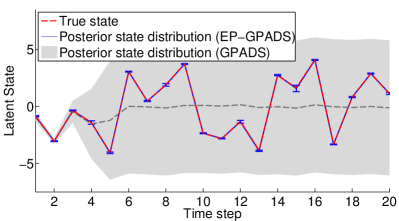
(a) Example trajectory distributions with 95% confidence bounds.

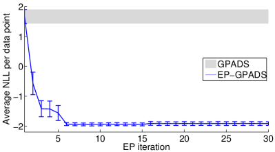
(b) Average NLL_x as a function of the EP iteration with twice the standard error.

Figure 2: 2(a) Posterior latent state distributions using EP-GPADS (blue) and the GPADS (gray). The ground truth is shown in red (dashed). The GPADS quickly loses track of the period of the state revealed by the large posterior uncertainty. EP with moment matching (EP-GPADS) in the GPDS iteratively refines the GPADS posterior and can closely follow the true latent state trajectory. 2(b) Average NLL_x per data point in latent space with standard errors of the posterior state distributions computed by the GPADS and the EP-GPADS as a function of EP iterations.

4.2 Pendulum Tracking

We considered a pendulum tracking problem to demonstrate GPDS inference in multidimensional settings, as well as the ability to handle control inputs. The state $\boldsymbol{x}$ of the system is given by the angle $\phi$ measured from being upright and the angular velocity $\dot{\phi}$. The pendulum used has a mass of $1\,\mathrm{kg}$ and a length of $1\,\mathrm{m}$, and random torques $u\in[-2,2]\,\mathrm{Nm}$ were applied for a duration $200\,\mathrm{ms}$ (zero-order-hold control). The system noise covariance was set to $\boldsymbol{\Sigma}_{w}=\mathrm{diag}(0.3^{2},0.1^{2}).$ The state was measured indirectly by two bearings sensors with coordinates $(x_{1},y_{1})=(-2,0)$ and $(x_{2},y_{2})=(-0.5,-0.5)$, respectively, according to $\boldsymbol{z}=[z_{1},z_{2}]^{\top}+\boldsymbol{v}\,,\,\,\boldsymbol{v}\sim\mathcal{N}\left(\boldsymbol{0},\mathrm{diag}(0.1^{2},0.05^{2})\right)$ with $z_{i}=\arctan\big{(}\tfrac{\sin\phi-y_{i}}{\cos\phi-x_{i}}\big{)}$, $i=1,2$. We trained the GP models using 4 randomly generated trajectories of length $T=20$ time steps, starting from an initial state distribution $p(\boldsymbol{x}_{1})=\mathcal{N}(\boldsymbol{0},\mathrm{diag}(\pi^{2}/16^{2},0.5^{2}))$ around the upright position. For testing, we generated 12 random trajectories starting from $p(\boldsymbol{x}_{1})$.

Table 2: Performance comparison on the pendulum-swing data. Lower values are better.

	NLLx	MAEx	NLLz
GPEKS	${\color[rgb]{1,0,0}\bf-0.35\pm 0.39}$	$0.30\pm 0.02$	$-2.41\pm 0.047$
EP-GPEKS	${\color[rgb]{1,0,0}\bf-0.33\pm 0.44}$	$0.31\pm 0.02$	$-2.39\pm 0.038$
GPADS	${\color[rgb]{0,0,1}\bf-0.80\pm 0.06}$	$0.30\pm 0.02$	$-2.37\pm 0.042$
EP-GPADS	${\color[rgb]{0,0,1}\bf-0.85\pm 0.05}$	$0.29\pm 0.02$	$-2.40\pm 0.037$

Tab. 2 summarizes the performance of the various inference methods. Generally, the (EP-)GPADS performed better than the (EP-)GPEKS across all performance measures. This indicates that the (EP-)GPEKS suffered from overconfident posteriors compared to (EP-)GPADS, which is especially pronounced in the degrading NLL_x values with increasing EP iterations and the relatively high standard errors. In about 20% of the test cases, the inference methods based on explicit linearization of the posterior mean function (GPEKS and EP-GPEKS) ran into numerical problems typical of linearizations [6], i.e., overconfident posterior distributions that caused numerical problems. We excluded these runs from the results in Tab. 2. The inference algorithms based on moment matching (GPADS and EP-GPADS) were numerically stable as their predictions are typically more coherent due to conservative approximations of moment matching.

4.3 Motion Capture Data

We considered motion capture data (from http://mocap.cs.cmu.edu/, subject 64) containing 10 trials of golf swings recorded at $120\,\mathrm{Hz}$, which we subsampled to $20\,\mathrm{Hz}$. After removing observation dimensions with no variability we were left with observations $\boldsymbol{z}_{t}\in\mathds{R}^{56}$, which were then whitened as a pre-processing step. For trials 1–7 (403 data points), we used the GPDM [21] to learn MAP estimates of the latent states $\boldsymbol{x}_{t}\in\mathds{R}^{3}$. These estimated latent states and their corresponding observations are used to train the GP models $\mathcal{GP}_{f}$ and $\mathcal{GP}_{g}$. Trials 8–10 were used as test data without ground truth labels. The GPDM [21] focuses on learning a GPDS; we are interested in good approximate inference in these models.

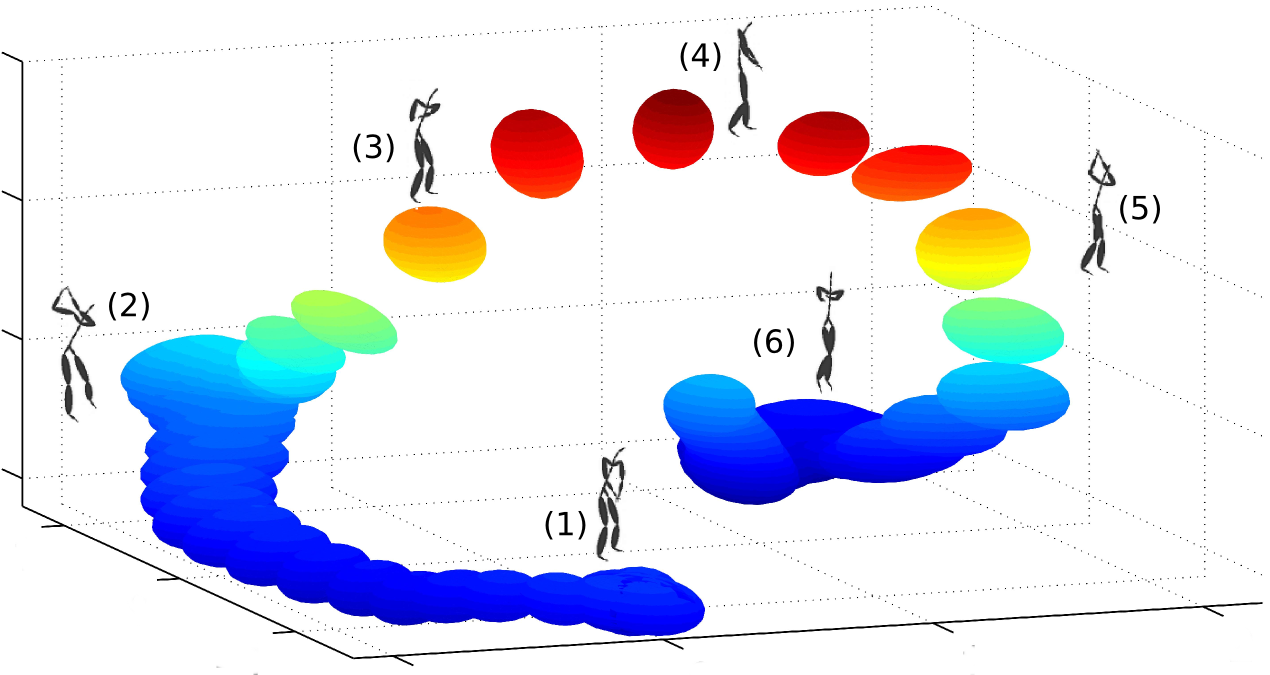
Figure 3: Latent space posterior distribution (95% confidence ellipsoids) of a test trajectory of the golf-swing motion capture data. The further the ellipsoids are separated the faster the movement.

Fig. 3 shows the latent-state posterior distribution of a single test sequence (trial 10) obtained from the EP-GPADS. The most significant prediction errors in observed space occurred in the region corresponding to the yellow/red ellipsoids, which is a low-dimensional embedding of the motion when the golf player hits the ball, i.e., the periods of high acceleration (poses 3–5).

Tab. 3 summarizes the results of inference on the golf data set in all test trials: Iterating forward-backward smoothing by means of EP improved the inferred posterior distributions over the latent states. The posterior distributions in latent space inferred by the EP-GPEKS were tighter than the ones inferred by the EP-GPADS. The NLL_z-values suffered a bit from this overconfidence, but the predictive performance of the EP-GPADS and EP-GPEKS were similar. Generally, inference was more difficult in areas with fast movements (poses 3–5 in Fig. 3) where training data were sparse.

Table 3: Average inference performance (NLL_z, motion capture data set). Lower values are better.

Test trial	GPEKS	EP-GPEKS	GPADS	EP-GPADS
Trial 8	14.20	13.82	14.28	14.09
Trial 9	15.63	14.71	15.19	14.84
Trial 10	26.68	25.73	25.64	25.42

The computational demand the two inference methods for GPDSs we presented is vastly different. High-dimensional approximate inference in the motion capture example using moment matching (EP-GPADS) was about two orders of magnitude slower than approximate inference based on linearization of the posterior GP mean (EP-GPEKS): For updating the posterior and the messages for a single time slice, the EP-GPEKS required less than $0.5\,\mathrm{s}$, the EP-GPADS took about $20\,\mathrm{s}$. Hence, numerical stability and more coherent posterior inference with the EP-GPADS trade off against computational demands.

5 Conclusion

We have presented an approximate message passing algorithm based on EP for improved inference and Bayesian state estimation in GP dynamical systems. Our message-passing formulation generalizes current inference methods in GPDSs to iterative forward-backward smoothing. This generalization allows for improved predictions and comprises existing methods for inference in the wider theory for dynamical systems as a special case. Our new inference approach makes the full power of the GPDS model available for the study of complex time-series data. Future work includes investigating alternatives to linearization and moment matching when computing messages, and the more general problem of learning in Gaussian process dynamical systems.

Appendix A GP Predictions from Test Input Distributions

We will now review two approximations to the predictive distribution

$$p(\boldsymbol{x}_{t})=\iint p(f(\boldsymbol{x}_{t-1})|\boldsymbol{x}_{t-1})p(\boldsymbol{x}_{t-1})\mathrm{d}f\mathrm{d}\boldsymbol{x}_{t-1}\,,$$ (18)

where $f\sim\mathcal{GP}$ and $\boldsymbol{x}_{t-1}\sim\mathcal{N}(\boldsymbol{\mu}_{t-1},\boldsymbol{\Sigma}_{t-1})$.

A.1 Moment Matching

In the moment-matching approach, we analytically compute the mean $\boldsymbol{\mu}_{t}$ and the covariance $\boldsymbol{\Sigma}_{t}$ of $p(\boldsymbol{x}_{t})$. Using the law of iterated expectations, we obtain

$$\boldsymbol{\mu}_{t}=\mathds{E}_{\boldsymbol{x}_{t-1}}\big{[}\mathds{E}_{f}[f(\boldsymbol{x}_{t-1})|\boldsymbol{x}_{t-1}]\big{]}=\mathds{E}_{\boldsymbol{x}_{t-1}}[m_{f}(\boldsymbol{x}_{t-1})]\,,$$ (19)

where $m_{f}$ is the posterior mean function of the dynamics GP. For target dimension $a=1,\dotsc,D$, we obtain

$$\boldsymbol{\mu}_{t}^{a} =\boldsymbol{q}_{a}^{\top}\boldsymbol{\beta}_{a}\,,\quad q_{a_{i}}=\tfrac{\sigma_{f}^{2}}{\sqrt{|\boldsymbol{\Sigma}_{t-1}\boldsymbol{\Lambda}_{a}^{-1}+\boldsymbol{I}|}}\exp\big{(}-\tfrac{1}{2}\boldsymbol{\nu}_{i}^{\top}(\boldsymbol{\Sigma}_{t-1}+\boldsymbol{\Lambda}_{a})^{-1}\boldsymbol{\nu}_{i}\big{)}\,,\quad\boldsymbol{\nu}_{i}\coloneqq(\boldsymbol{x}_{i}-\boldsymbol{\mu}_{t-1})$$ (20)

for $i=1,\dotsc,n$, where $\boldsymbol{\beta}_{a}=\boldsymbol{K}_{a}^{-1}\boldsymbol{y}_{a}$.

Using the law of iterated variances, the entries of $\boldsymbol{\Sigma}_{t}$ for target dimensions $a,b=1,\dotsc,D$ are

$$\sigma_{aa}^{2} \!=\!\mathds{E}_{\boldsymbol{x}_{t-1}}\big{[}\mathrm{var}_{f}[\Delta_{a}|\boldsymbol{x}_{t-1}]\big{]}\!+\!\mathds{E}_{f,\boldsymbol{x}_{t-1}}[\Delta_{a}^{2}]\!-\!(\boldsymbol{\mu}_{t}^{a})^{2},$$ (21)

$$\sigma_{ab}^{2} \!=\!\mathds{E}_{f,\boldsymbol{x}_{t-1}}[\Delta_{a}\Delta_{b}]\!-\!\boldsymbol{\mu}_{t}^{a}\boldsymbol{\mu}_{t}^{b}\,,\quad a\neq b\,,$$ (22)

respectively, where $\mu_{t}^{a}$ is known from (20). The off-diagonal terms $\sigma_{ab}^{2}$ do not contain an additional term $\mathds{E}_{\boldsymbol{x}_{t-1}}[\mathrm{cov}_{f}[\Delta_{a},\Delta_{b}|\boldsymbol{x}_{t-1}]]$ because of the conditional independence assumption used for GP training: Target dimensions do not covary for a given $\boldsymbol{x}_{t-1}$.

For the term common to both $\sigma_{aa}^{2}$ and $\sigma_{ab}^{2}$, we obtain

$$\mathds{E}_{f,\boldsymbol{x}_{t-1}}[\Delta_{a}\Delta_{b}]=\boldsymbol{\beta}_{a}^{\top}\boldsymbol{Q}\boldsymbol{\beta}_{b}\,,\qquad Q_{ij}\!=\!\tfrac{k_{a}(\boldsymbol{x}_{i},{\boldsymbol{\mu}}_{t-1})k_{b}(\boldsymbol{x}_{j},{\boldsymbol{\mu}}_{t-1})}{\sqrt{|\boldsymbol{R}|}}\exp\big{(}\tfrac{1}{2}\boldsymbol{z}_{ij}^{\top}\boldsymbol{R}^{-1}{\boldsymbol{\Sigma}}_{t-1}\boldsymbol{z}_{ij}\big{)}$$ (23)

with $\boldsymbol{R}\coloneqq{\boldsymbol{\Sigma}}_{t-1}(\boldsymbol{\Lambda}_{a}^{-1}+\boldsymbol{\Lambda}_{b}^{-1})+\boldsymbol{I}$ and $\boldsymbol{z}_{ij}\coloneqq\boldsymbol{\Lambda}_{a}^{-1}\boldsymbol{\nu}_{i}+\boldsymbol{\Lambda}_{b}^{-1}\boldsymbol{\nu}_{j}$ with $\boldsymbol{\nu}_{i}$ taken from (20). Hence, the off-diagonal entries $\sigma_{ab}^{2}$ of $\boldsymbol{\Sigma}_{t}$ are fully determined by (20) and (22).

From (21), we see that the diagonal entries $\sigma_{aa}^{2}$ of $\boldsymbol{\Sigma}_{t}$ contain an additional term

$$\mathds{E}_{\boldsymbol{x}_{t-1}}\big{[}\mathrm{var}_{f}[\Delta_{a}|\boldsymbol{x}_{t-1}]\big{]} =\sigma_{f_{a}}^{2}-\mathrm{Tr}\big{(}\boldsymbol{K}_{a}^{-1}\boldsymbol{Q}\big{)}+\sigma_{w_{a}}^{2}$$ (24)

with $\boldsymbol{Q}$ given in (23). This concludes the computation of $\boldsymbol{\Sigma}_{t}$.

The moment-matching approximation minimizes the KL divergence KL$(p||q)$ between the true distribution $p$ and an approximate Gaussian distribution $q$. This is generally a conservative approximation, i.e., $q$ has probability mass where $p$ has mass [2].

A.2 Linearizing the GP Mean Function

An alternative way of approximating the predictive GP distribution for uncertain test inputs is to linearize the posterior GP mean function [9]. This is equivalent to computing the expected linearization of the GP distribution over functions. Given this linearized function, we apply standard results for mapping Gaussian distributions through linear models. Linearizing the posterior GP mean function yields to a predicted mean that corresponds to the posterior GP mean function evaluated at the mean of the input distribution, i.e.,

$$\boldsymbol{\mu}_{t}^{a} =\mathds{E}_{f}[f_{a}(\boldsymbol{\mu}_{t-1})]=\boldsymbol{r}_{a}^{\top}\boldsymbol{\beta}_{a}\,,\qquad r_{a_{i}}=\sigma_{f_{a}}^{2}\exp\big{(}-\tfrac{1}{2}(\boldsymbol{x}_{i}-{\boldsymbol{\mu}}_{t-1})^{\top}\boldsymbol{\Lambda}_{a}^{-1}(\boldsymbol{x}_{i}-{\boldsymbol{\mu}}_{t-1})\big{)}$$ (25)

for $i=1,\dotsc,n$ and target dimensions $a=1,\dotsc,D$, where $\boldsymbol{\beta}_{a}=\boldsymbol{K}_{a}^{-1}\boldsymbol{y}_{a}$. The covariance matrix $\boldsymbol{\Sigma}_{t}$ of the GP prediction is

$$\boldsymbol{\Sigma}_{t} =\boldsymbol{V}{\boldsymbol{\Sigma}}_{t-1}\boldsymbol{V}^{\top}+\boldsymbol{\Sigma}_{w}\,,\qquad\boldsymbol{V}=\tfrac{\partial\boldsymbol{\mu}_{t}}{\partial{\boldsymbol{\mu}}_{t-1}}=\boldsymbol{\beta}_{a}^{\top}\tfrac{\partial\boldsymbol{r}_{a}}{\partial{\boldsymbol{\mu}}_{t-1}}\,,$$ (26)

where $\boldsymbol{r}_{a}$ is given in (25) and $\boldsymbol{V}$ is the Jacobian evaluated at $\boldsymbol{\mu}_{t-1}$. In (26), $\boldsymbol{\Sigma}_{w}$ is a diagonal matrix whose entries are the model uncertainty plus the noise variance evaluated at ${\boldsymbol{\mu}}_{t-1}$. This means “model uncertainty” no longer depends on the density of the data points. Instead it is assumed constant.

Using linearization, the approximation optimality in the KL sense of the moment matching is lost. However, especially in high dimensions, linearization is computationally more beneficial. This speedup is largely due to the simplified treatment of model uncertainty.

References

- [1] B. D. O. Anderson and J. B. Moore. Optimal Filtering. Dover Publications, Mineola, NY, USA, 2005.
- [2] C. M. Bishop. Pattern Recognition and Machine Learning. Information Science and Statistics. Springer-Verlag, 2006.
- [3] A. Damianou, M. K. Titsias, and N. D. Lawrence. Variational Gaussian Process Dynamical Systems. In Advances in Neural Information Processing Systems, 2011.
- [4] M. P. Deisenroth, M. F. Huber, and U. D. Hanebeck. Analytic Moment-based Gaussian Process Filtering. In L. Bouttou and M. L. Littman, editors, Proceedings of the 26th International Conference on Machine Learning, pages 225–232, Montreal, QC, Canada, June 2009. Omnipress.
- [5] M. P. Deisenroth and S. Mohamed. Expectation Propagation in Gaussian Process Dynamical Systems. In Advances in Neural Information Processing Systems, 2012.
- [6] M. P. Deisenroth, R. Turner, M. Huber, U. D. Hanebeck, and C. E. Rasmussen. Robust Filtering and Smoothing with Gaussian Processes. IEEE Transactions on Automatic Control, 57(7):1865–1871, 2012. doi:10.1109/TAC.2011.2179426.
- [7] T. Heskes and O. Zoeter. Expectation Propagation for Approximate Inference in Dynamic Bayesian Networks. In A. Darwiche and N. Friedman, editors, Proceedings of the International Conference on Uncertainty in Artificial Intelligence, pages 216–233, 2002.
- [8] S. J. Julier and J. K. Uhlmann. Unscented Filtering and Nonlinear Estimation. Proceedings of the IEEE, 92(3):401–422, March 2004.
- [9] J. Ko and D. Fox. GP-BayesFilters: Bayesian Filtering using Gaussian Process Prediction and Observation Models. Autonomous Robots, 27(1):75–90, July 2009.
- [10] M. Kuss and C. E. Rasmussen. Assessing Approximate Inference for Binary Gaussian Process Classification. Journal of Machine Learning Research, 6:1679–1704, December 2005.
- [11] T. P. Minka. Expectation Propagation for Approximate Bayesian Inference. In J. S. Breese and D. Koller, editors, Proceedings of the 17th Conference on Uncertainty in Artificial Intelligence, pages 362–369, Seattle, WA, USA, August 2001. Morgan Kaufman Publishers.
- [12] T. P. Minka. A Family of Algorithms for Approximate Bayesian Inference. PhD thesis, Massachusetts Institute of Technology, Cambridge, MA, USA, January 2001.
- [13] T. P. Minka. EP: A Quick Reference. 2008.
- [14] Y. Qi and T. Minka. Expectation Propagation for Signal Detection in Flat-Fading Channels. In Proceedings of the IEEE International Symposium on Information Theory, 2003.
- [15] J. Quiñonero-Candela, A. Girard, J. Larsen, and C. E. Rasmussen. Propagation of Uncertainty in Bayesian Kernel Models—Application to Multiple-Step Ahead Forecasting. In IEEE International Conference on Acoustics, Speech and Signal Processing, volume 2, pages 701–704, April 2003.
- [16] C. E. Rasmussen and C. K. I. Williams. Gaussian Processes for Machine Learning. Adaptive Computation and Machine Learning. The MIT Press, Cambridge, MA, USA, 2006.
- [17] M. W. Seeger. Expectation Propagation for Exponential Families. Technical report, University of California Berkeley, 2005.
- [18] M. W. Seeger. Bayesian Inference and Optimal Design for the Sparse Linear Model. Journal of Machine Learning Research, 9:759–813, 2008.
- [19] M. Toussaint and C. Goerick. From Motor Learning to Interaction Learning in Robotics, chapter A Bayesian View on Motor Control and Planning, pages 227–252. Springer-Verlag, 2010.
- [20] R. Turner, M. P. Deisenroth, and C. E. Rasmussen. State-Space Inference and Learning with Gaussian Processes. In Y. W. Teh and M. Titterington, editors, Proceedings of the Thirteenth International Conference on Artificial Intelligence and Statistics, volume JMLR: W&CP 9, pages 868–875, May 2010.
- [21] J. M. Wang, D. J. Fleet, and A. Hertzmann. Gaussian Process Dynamical Models for Human Motion. IEEE Transactions on Pattern Analysis and Machine Intelligence, 30(2):283–298, 2008.