Maximum likelihood characterization of distributions

Abstract

A famous characterization theorem due to C.F. Gauss states that the maximum likelihood estimator (MLE) of the parameter in a location family is the sample mean for all samples of all sample sizes if and only if the family is Gaussian. There exist many extensions of this result in diverse directions, most of them focussing on location and scale families. In this paper, we propose a unified treatment of this literature by providing general MLE characterization theorems for one-parameter group families (with particular attention on location and scale parameters). In doing so, we provide tools for determining whether or not a given such family is MLE-characterizable, and, in case it is, we define the fundamental concept of minimal necessary sample size at which a given characterization holds. Many of the cornerstone references on this topic are retrieved and discussed in the light of our findings, and several new characterization theorems are provided. Of particular interest is that one part of our work, namely the introduction of so-called equivalence classes for MLE characterizations, is a modernized version of Daniel Bernoulli’s viewpoint on maximum likelihood estimation.

, and

1 Introduction

In probability and statistics, a characterization theorem occurs whenever a given law or a given class of laws is the only one which satisfies a certain property. While probabilistic characterization theorems are concerned with distributional aspects of (functions of) random variables, statistical characterization theorems rather deal with properties of statistics, that is, measurable functions of a set of independent random variables (observations) following a certain distribution. Examples of probabilistic characterization theorems include:

1. [-]

2. Stein-type characterizations of probability laws, inspired from the classical Stein and Chen characterizations of the normal and the Poisson distributions, see Stein [43], Chen [10];

3. maximum entropy characterizations, see Cover and Thomas [12], Chapter 11;

4. conditioning characterizations of probability laws such as, for example, determining the marginal distributions of the random components $X$ and $Y$ of the vector $(X,Y)^{\prime}$ if only the conditional distribution of $X$ given $X+Y$ is known, see Patil and Seshadri [37].

The class of statistical characterization theorems includes:

1. [-]

2. characterizations of probability distributions by means of order statistics, see Galambos [19] and Kotz [29] for an overview on the vast literature on this subject;

3. Cramér-type characterizations, see Cramér [13];

4. characterizations of probability laws by means of one linear statistic, of identically distributed statistics or of the independence between two statistics, see Lukacs [33].

Besides their evident mathematical interest per se, characterization theorems also provide a better understanding of the distributions under investigation and sometimes offer unexpected handles to innovations which might not have been uncovered otherwise. For instance, Chen and Stein’s characterizations are at the heart of the celebrated Stein’s method, see the recent Chen, Goldstein and Shao [11] and Ross [42] for an overview; maximum entropy characterizations are closely related to the development of important tools in information theory (see Akaike [2, 3]), Bayesian probability theory (see Jaynes [25]) or even econometrics (see Wu [48], Park and Bera [36]; characterizations of probability distributions by means of order statistics are, according to Teicher [46], “harbingers of […] characterization theorems”, and have been extensively studied around the middle of the twentieth century by the likes of Kac, Kagan, Linnik, Lukacs or Rao; Cramér-type characterizations are currently the object of active research, see Bourguin and Tudor [6]. This list is by no means exhaustive and for further information about characterization theorems as a whole, we refer to the extensive and still relevant monograph Kagan, Linnik and Rao [27], or to Kotz [29], Bondesson [5], Haikady [22] and the references therein.

In this paper, we focus on a family of characterization theorems which lie at the intersection between probabilistic and statistical characterizations, the so-called MLE characterizations.

1.1 A brief history of MLE characterizations

We call MLE characterization the characterization of a (family of) probability distribution(s) via the structure of the Maximum Likelihood Estimator (MLE) of a certain parameter of interest (location, scale, etc.).

The first occurrence of such a theorem is in Gauss [20], where Gauss showed that the normal (a.k.a. the Gaussian) is the only location family for which the sample mean $\bar{x}=n^{-1}\sum_{i=1}^{n}x_{i}$ is “always” the MLE of the location parameter. More specifically, Gauss [20] proved that, in a location family $g(x-\theta)$ with differentiable density $g$, the MLE for $\theta$ is the sample mean for all samples $\mathbf{x}^{(n)}=(x_{1},\ldots,x_{n})$ of all sample sizes $n$ if, and only if, $g(x)=\kappa_{\lambda}\mathrm{e}^{-\lambda x^{2}/2}$ for $\lambda>0$ some constant and $\kappa_{\lambda}$ the adequate normalizing constant. Discussed as early as in Poincaré [38], this important result, which we will throughout call Gauss’ MLE characterization, has attracted much attention over the past century and has spawned a spree of papers about MLE characterization theorems, the main contributions (extensions and improvements on different levels, see below) being due to Teicher [46], Ghosh and Rao [21], Kagan, Linnik and Rao [27], Findeisen [18], Marshall and Olkin [34] and Azzalini and Genton [4]. (See also Hürlimann [24] for an alternative approach to this topic.) For more information on Gauss’ original argument, we refer the reader to the accounts of Hald [23], pages 354 and 355, and Chatterjee [9], pages 225–227. See Norden [35] or the fascinating Stigler [45] for an interesting discussion on MLEs and the origins of this fundamental concept.

The successive refinements of Gauss’ MLE characterization contain improvements on two distinct levels. Firstly, several authors have worked towards weakening the regularity assumptions on the class of distributions considered; for instance, Gauss requires differentiability of $g$, while Teicher [46] only requires continuity. Secondly, many authors have aimed at lowering the sample size necessary for the characterization to hold (i.e., the “always”-statement); for instance, Gauss requires that the sample mean be MLE for the location parameter for all sample sizes simultaneously, Teicher [46] only requires that it be MLE for samples of sizes 2 and 3 at the same time, while Azzalini and Genton [4] only need that it be so for a single fixed sample size $n\geq 3$. Note that Azzalini and Genton [4] also construct explicit examples of non-Gaussian distributions for which the sample mean is the MLE of the location parameter for the sample size $n=2$. We already draw the reader’s attention to the fact that Azzalini and Genton’s [4] result does not supersede Teicher’s [46], since the former require more stringent conditions (namely differentiability of the $g$’s) than the latter. We will provide a more detailed discussion on this interesting fact again at the end of Section 4.

Aside from these “technical” improvements, the literature on MLE characterization theorems also contains evolutions in different directions which have resulted in a new stream of research, namely that of discovering new (i.e., different from Gauss’ MLE characterization) MLE characterization theorems. These can be subdivided into two categories. On the one hand, MLE characterizations with respect to the location parameter but for other forms than the sample mean have been shown to hold for densities other than the Gaussian. On the other hand, MLE characterizations with respect to other parameters of interest than the location parameter have also been considered. Teicher [46] shows that if, under some regularity assumptions and for all sample sizes, the MLE for the scale parameter of a scale target distribution is the sample mean $\bar{x}$ then the target is the exponential distribution, while if it corresponds to the square root of the sample arithmetic mean of squares $(\frac{1}{n}\sum_{i=1}^{n}x_{i}^{2})^{1/2}$, then the target is the standard normal distribution. Following suit on Teicher’s work, Kagan, Linnik and Rao [27] establish that the sample median is the MLE for the location parameter for all samples of size $n=4$ if and only if the parent distribution is the Laplace law. Also, in Ghosh and Rao [21], it is shown that there exist distributions other than the Laplace for which the sample median at $n=2$ or $n=3$ is MLE. Ferguson [17] generalizes Teicher’s [46] location-based MLE characterization from the Gaussian to a one-parameter generalized normal distribution, and Marshall and Olkin [34] generalize Teicher’s [46] scale-based MLE characterization of the exponential distribution to the gamma distribution with shape parameter $\alpha>0$ by replacing $\bar{x}$ as MLE for the scale parameter with $\bar{x}/\alpha$.

There also exist contributions by Buczolich and Székely [7] where they investigate situations in which a weighted average of ordered sample elements can be an MLE of the location parameter. MLE characterizations in the multivariate setup have been proposed, inter alia, in Marshall and Olkin [34] and Azzalini and Genton [4]. In parallel to all these “linear” MLE characterizations there have also been a number of developments regarding MLE characterizations for spherical distributions, that is distributions taking their values only on the unit hypersphere in higher dimensions, see Duerinckx and Ley [16] and the references therein.

Finally, there exists a different stream of MLE characterization research, inspired by Poincaré [38], in which one relaxes the assumptions made on the role of the parameter $\theta$ and seeks to understand the conditions under which the MLE for this $\theta$ is an arithmetic mean. This approach to MLE characterization theorems is known as Gauss’ principle; quoting Campbell [8] “by Gauss’ principle we shall mean that a distribution should be chosen so that the maximum likelihood estimate of the parameter $\theta$ is the same as the arithmetic mean estimate given by $n^{-1}\sum_{k=1}^{n}T(x_{k})$”, with $\theta={\mathrm{E}}(T(X))$ for some known function $T$. When $T$ is the identity function and one considers one-parameter location families then we recover the MLE characterization problem solved by Gauss [20]. For general one-parameter families the corresponding problem was solved in Poincaré [38]. Campbell [8] broadens Poincaré’s conclusion to general functions $T$ and to the multivariate setup, while Bondesson [5] further extends the above works to exponential families with nuisance parameters. As pointed out by their authors, many of these results remain valid for discrete distributions; for other MLE characterizations of discrete probability laws, we also refer to Puig [39] and Puig and Valero [41].

1.2 Applications of MLE characterizations

Perhaps the most remarkable application of MLE characterizations is to be found in the very origins of this field of study, whose forefathers sought to define families of probability distributions which were “natural” for a given important problem. For instance, the Gaussian distribution was uncovered by Gauss through his effort of finding the location family for which the sample mean $\bar{x}$ is a most probable value for $\theta$, the location parameter. Similarly, Poincaré in his “Calcul des Probabilités” (2nd ed., 1912) derived in Chapter 10 (pages 147–168 in the 1896 edition) a particular case of the exponential families of distributions (see Lehmann and Casella [30], Section 1.5) by asking for which distributions $\bar{x}$ is the MLE of $\theta$, without specifying the role of the parameter. We refer to the historical remarks at the end of Bondesson [5] and the references therein for more information on both the works of Gauss and Poincaré. Following Gauss’ ideas, von Mises [47] defined the circular (i.e., spherical in dimension two) analogue of the Gaussian distribution by looking for the circular distribution whose circular location parameter always has the circular sample mean as MLE; this led to the now famous Fisher–von Mises–Langevin (abbreviated FvML) distribution on spheres.

Of an entirely different nature is Campbell’s [8] use of MLE characterizations. In his paper, Campbell establishes an equivalence between MLE characterizations in the spirit of Gauss’ principle and the minimum discrimination information estimation of probabilities. More recently, Puig [40] has applied MLE characterizations in order to characterize the Harmonic Law as the only statistical model on the positive real half-line that satisfies a certain number of requirements. As a last example, we cite the work of Ley and Paindaveine [32] who solved a long-standing problem on skew-symmetric distributions through an argument resting on Gauss’ MLE characterization.

1.3 Purpose of the paper

As is perhaps intuitively clear, many of the results on MLE characterizations stem from a common origin. As a matter of fact many authors often follow the same “smart path” that can be summarized in three steps: (a) choose the role of the parameter of interest $\theta$ (location or scale); (b) choose a remarkable form for the MLE for $\theta$ (e.g., sample mean, variance or median); (c) use the freedom of choice in the samples as well as the sample size (two samples of respective sizes 2 and 3, one sample of size 3, all samples of all sizes$,\ldots$) to obtain the largest class of distributions satisfying certain assumptions (continuous at a single point, continuous, differentiable$,\ldots$) which share this specific MLE. While similar, the arguments leading to the different results nevertheless are largely ad hoc and rest upon crafty manipulations of the explicit given form of the MLE. Moreover, step (c) contains assumptions on the minimal sample size and on the properties of the distributions being characterized, the necessity of which is barely addressed.

The purpose of the present paper is to unify this important literature by explaining the mechanism behind this “smart path” in the more general context of one-parameter group families (as defined in Section 6) although still with particular focus on location and scale families. In doing so, we will introduce the concept of minimal covering sample size (MCSS), a quantity whose value depends on the structure of the support of the target distribution and from which one deduces the a priori minimal necessary sample size (MNSS) at which an MLE characterization holds for a given family of distributions (see Duerinckx and Ley [16] where this notion was introduced). As we shall see, the MCSS and MNSS explain many of the differences in the “always”-statements appearing throughout the literature on MLE characterization. Moreover our unified perspective on MLE characterizations not only permits to identify the minimal sufficient conditions under which group families are characterized by their MLEs (MLE-characterizable) but also provide tools for (easily) constructing new MLE characterizations of many important families of distributions.

In a nutshell, our goal is to (i) propose a unified perspective on MLE characterizations for one-parameter group families, (ii) answer the question of which such families are MLE-characterizable and find their MNSS, (iii) retrieve, improve on and better understand existing results via our general analysis, and (iv) construct new MLE characterization results. Our contribution to the important literature on MLE characterizations unifies the cornerstone references Teicher [46], Ferguson [17], Kagan, Linnik and Rao [27], Marshall and Olkin [34], Azzalini and Genton [4] (to cite but these) and complements the understanding brought by the seminal works of Poincaré [38], Campbell [8] and Bondesson [5].

1.4 Outline of the paper

In Section 2 we describe the framework of our study, give all necessary notations and introduce the so-called equivalence classes. In Section 3 we establish and interpret the above-mentioned notion of MCSS which will be central to this paper. In Section 4, we derive the MLE characterization for univariate location families, while in Section 5 we proceed in a similar way with univariate scale families. In Section 6 we obtain MLE characterizations for general one-parameter group families, allowing us to study other roles of the parameter (e.g., skewness). In Section 7 we apply our findings to particular families of distributions. We conclude the paper with a discussion, in Section 8, of the different possible extensions that are yet to be explored.

2 Notations and generalities on ML estimators, equivalence classes

Throughout we consider observations $\mathbf{X}^{(n)}=(X_{1},X_{2},\ldots,X_{n})$ that are sampled independently from a distribution $P_{\theta}^{f}$ (with density $f$) which we suppose to be entirely known up to a parameter $\theta\in\Theta\subset\mathbb{R}$. The true parameter value $\theta_{0}\in\Theta$ is estimated by ML estimation on basis of $\mathbf{X}^{(n)}$. As explained in the Introduction, our aim consists in determining which classes of distributions are identifiable by means of the MLE of the parameter of interest $\theta$, a parameter that can, in principle, be of any nature (i.e., location, scale, etc.). On the target family of distributions $\{P_{\theta}^{f}\mathchoice{\nobreak\,\colon}{\nobreak\,\colon}{\nobreak\,\colon\;}{\nobreak\,\colon\;}\theta\in\Theta\}$ we make the following general assumptions:

1. [-]

2. (A1) The parameter space $\Theta$ contains an open set $\Theta_{0}$ of which the true parameter $\theta_{0}$ is an interior point.

3. (A2) For each $\theta\in\Theta_{0}$, the distribution $P_{\theta}^{f}$ has support $S$ independent of $\theta$.

4. (A3) For all $1\leq i\leq n$ the random variable $X_{i}$ has a density $f(x_{i};\theta)$ with respect to the (dominating) Lebesgue measure.

5. (A4) For $\theta\neq\theta^{\prime}\in\Theta_{0}$, we have $P_{\theta}^{f}\neq P_{\theta^{\prime}}^{f}$.

These assumptions are taken from Lehmann and Casella [30], page 444.

Remark 2.1.

Although typically we will be concerned with either location families with densities of the form $f(x;\theta)=f(x-\theta)$ for $\theta\in\mathbb{R}$ the location parameter, or scale families with densities of the form $f(x;\theta)=\theta f(x\theta)$ for $\theta\in\mathbb{R}^{+}_{0}$ the scale parameter, other roles for $\theta$ (skewness, tail behavior…) can also be considered; see Section 6 where we detail our approach for one-parameter group families.

Remark 2.2.

While throughout the paper we restrict our attention to the univariate setting, it is easy to see that our arguments are in some cases transposable word-by-word to the multivariate case. We discuss this matter briefly in Section 8.

Remark 2.3.

Assumption (A2) implies that only densities with full support $\mathbb{R}$ may be considered for ML estimation of a location parameter, while only densities with support either $\mathbb{R}$, $\mathbb{R}^{+}$ or $\mathbb{R}^{-}$ may be considered for ML estimation of a scale parameter. Despite the fact that these restrictions are natural in the present context they can, if deemed necessary, be lifted. We will briefly discuss this topic in Section 8.

We define, for a fixed sample size $n\geq 1$, the MLE of the parameter $\theta$ as (if it exists) the measurable function

$$\hat{\theta}^{(n)}_{f}\mathchoice{\nobreak\,\colon}{\nobreak\,\colon}{\nobreak\,\colon\;}{\nobreak\,\colon\;}S^{n}:=S\times\cdots\times S\to\Theta_{0}\mathchoice{\nobreak\,\colon}{\nobreak\,\colon}{\nobreak\,\colon\;}{\nobreak\,\colon\;}\mathbf{x}^{(n)}:=(x_{1},\ldots,x_{n})\mapsto\hat{\theta}^{(n)}_{f}\bigl{(}\mathbf{x}^{(n)}\bigr{)}$$

for which

$$\prod_{i=1}^{n}f\bigl{(}x_{i};\hat{\theta}^{(n)}_{f}\bigl{(}\mathbf{x}^{(n)}\bigr{)}\bigr{)}\geq\prod_{i=1}^{n}f(x_{i};\theta)$$ (1)

for all $\theta\in\Theta_{0}$ and all samples $\mathbf{x}^{(n)}\in S^{n}$ of size $n$. It is not trivial to provide minimal conditions on $f$ under which $\hat{\theta}^{(n)}_{f}(\mathbf{x}^{(n)})$ exists, is uniquely defined and satisfies the necessary measurability conditions. Consistency of the MLE is also a delicate matter and further regularity conditions are required for the problem to make sense. As in Cramér [14, 15] one may suppose that, for almost all $x$, the density $f(x;\theta)$ is differentiable with respect to $\theta$. This allows to define the MLE as the solution of the local likelihood equation

$$\sum_{i=1}^{n}\varphi_{f}(x_{i};\theta)=0,$$ (2)

where

$$\varphi_{f}(x;\theta):=\frac{\partial}{\partial\theta}\log f(x;\theta)$$

is the score function of the density $f$ associated with the parameter $\theta$ (we set this function to 0 outside the support of $f$). The solution to (2) has, at least asymptotically, the required properties (see Lehmann and Casella [30], Theorem 6.3.7). Furthermore, this way of proceeding allows for a simple sufficient condition for uniqueness of the MLE: the mapping $x\mapsto\varphi_{f}(x;\theta)$ has to be strictly monotone and to cross the $x$-axis. Note that this requirement coincides with strong unimodality or log-concavity of the density $f$ when $\theta$ is a location parameter (see Lehmann and Casella [30], Exercise 6.3.15).

Remark 2.4.

Although in general there is no explicit expression for the MLE of a given parametric family, there exist several important distributions that not only satisfy all the above requirements but also allow for MLEs which take on a remarkable form. Taking $f=\phi$ the standard normal density, the MLE for the location parameter is $\bar{x}:=\frac{1}{n}\sum_{i=1}^{n}x_{i}$, the sample arithmetic mean, while that for the scale parameter is $(\frac{1}{n}\sum_{i=1}^{n}x_{i}^{2})^{1/2}$, the square root of the sample arithmetic mean of squares. Taking $f$ the exponential density, the MLE for the scale parameter becomes $\bar{x}$.

As outlined in Section 1.3, our objective in this paper is to determine minimal conditions under which a given form of MLE for a given type of parameter identifies a specific probability distribution. Upon making this statement there immediately arises a trivial identification problem (due to our definition of maximum likelihood estimators) which we first need to evacuate. Indeed if $\hat{\theta}_{f}^{(n)}$ maximizes the $f$-likelihood function, then it also maximizes the $g$-likelihood function for any function $g=cf^{d}$ with $d>0$ and $c$ a normalizing constant. In fact, from our definitions (1) and (2), it is immediate that any two parametric densities $f(x;\theta)$ and $g(x;\theta)$ with same support $S$ and such that

$$\varphi_{g}(x;\theta)=d\varphi_{f}(x;\theta)\qquad\forall x\in S$$ (3)

for some $d>0$ share the same MLE for $\theta$. This seemingly trivial and innocuous observation leads us to the introduction of a concept that happens to be fundamental for this paper and for MLE characterizations in general: the concept of (parameter-dependent) equivalence classes (e.c. hereafter), meaning that two densities are equivalent if their score functions satisfy (3). It is obvious that e.c.’s constitute a partition of the space of distributions. Stated simply, without further conditions or specifications on the density associated with the target distribution $P_{\theta}^{f}$ (the target density $f$) and on the functions $g$, MLE characterization theorems identify an e.c. of distributions rather than a single well-specified distribution.

Remark 2.5.

Considering, for example, Gauss’ MLE characterization, both Teicher [46] and Azzalini and Genton [4], to cite but these, identify the Gaussian distribution with respect to its location parameter only up to an unknown variance. On the contrary, when dealing with scale characterizations, Teicher [46] imposes a tail-constraint in order to be able to single out the standard exponential and the standard Gaussian distribution.

The use of e.c.’s are far from new in the context of ML estimation. Indeed Daniel Bernoulli, who is considered to be one of the first authors to introduce the idea underlying the concept of maximum likelihood, noted as early as in 1778 that the roots of his “likelihood function” would not change by squaring the semi-circular density he used (see Stigler [44], Chapter 16). Further ideas of Bernoulli can be found in Kendall [28], Section 19, and they clearly demonstrate that the equivalence (3) can be viewed as a modern expression of Bernoulli’s early thoughts.

In what follows, we shall state our results in the most general possible way, without (at least in the main results) considering additional identification constraints. As will become clear from the subsequent sections, the nature of the parameter of interest $\theta$ heavily influences the partition of the space of distributions, so that, for each type of parameter, one needs to identify the e.c.’s (see the beginnings of Sections 4 and 5 for an illustration).

The framework we have developed so far allows us to reformulate the question underpinning the present article in a more transparent form, namely “Do there exist two distinct e.c.’s $\mathcal{F}(\theta)$ and $\mathcal{G}(\theta)$ such that the distributions $P_{\theta}^{f}$ and $P_{\theta}^{g}$ for $f\in\mathcal{F}(\theta)$ and $g\in\mathcal{G}(\theta)$ share a given MLE of the parameter of interest $\theta$”? As is perhaps already clear, the answer to this question is negative – at least in the interesting cases. To see why this ought to be the case let $\mathcal{F}(\theta)$ and $\mathcal{G}(\theta)$ be two e.c.’s which share an MLE for some sample size $n\geq 1$, in other words suppose that, for some $n\geq 1$, some $f\in\mathcal{F}(\theta)$ and some $g\in\mathcal{G}(\theta)$, the estimator $\hat{\theta}^{(n)}_{g}$ coincides with $\hat{\theta}^{(n)}_{f}$, that is,

$$\sum_{i=1}^{n}\log g\bigl{(}x_{i};\hat{\theta}^{(n)}_{f}\bigl{(}\mathbf{x}^{(n)}\bigr{)}\bigr{)}\geq\sum_{i=1}^{n}\log g(x_{i};\theta)$$ (4)

for all $\theta\in\Theta_{0}$ and all samples $\mathbf{x}^{(n)}\in S^{n}$ of size $n$. Then clearly the only way for $f$ and $g$ to satisfy (4) for all samples of size $n$ is that they be strongly related to one another; as we will see, under reasonable conditions, one can go one step further and deduce that if (4) holds true for a “sufficiently large $n$” then $f$ and $g$ must belong to the same e.c. This intuition is the heart of all the literature on MLE characterizations.

3 The minimal covering sample size

The first step towards establishing our general MLE characterizations is to gain a better understanding of the meaning of “sufficiently large $n$” for (4) to induce a characterization theorem. We use the notation $H_{n}$ to denote the hyperplane

$$H_{n}=\Biggl{\{}\mathbf{b}^{(n)}=(b_{1},\ldots,b_{n})\in\mathbb{R}^{n}\bigg{|}\sum_{j=1}^{n}b_{j}=0\Biggr{\}}$$

and associate, with any parametric distribution $P_{\theta}^{f}$ satisfying the requirements of Section 2, the collection(s) of sets

$$B_{n}^{f,\theta}(A)=\bigl{\{}\mathbf{b}^{(n)}\in H_{n}|\exists\mathbf{x}^{(n)}\in A^{n}\mbox{ with }b_{j}=\varphi_{f}(x_{j};\theta)\mbox{ for all }1\leq j\leq n\bigr{\}},$$ (5)

where $A^{n}=A\times\cdots\times A$ is the $n$-fold cartesian product of $A\subseteq S$, the support of the target $f$, and $\theta\in\Theta_{0}$. The interplay between the sets $B_{n}^{f,\theta}$ and the hyperplanes $H_{n}$ determines the minimal sample size $n$ for a characterization theorem to hold. The following lemma is crucial to our approach.

Lemma 3.1

Suppose that for some $\theta\in\Theta_{0}$ the mapping $x\mapsto\varphi_{f}(x;\theta)$ is strictly monotone over some interval $\mathcal{X}\subset S$ and that the (restricted) image $\mathcal{I}_{f,\theta}(\mathcal{X}):=\{\varphi_{f}(x;\theta)|x\in\mathcal{X}\}$ is of the form $(-P^{-}_{f,\theta},P^{+}_{f,\theta})$, for positive constants $P^{-}_{f,\theta},P^{+}_{f,\theta}$ (possibly infinite). Then, for all $n\geq 1$, $B_{n}^{f,\theta}(\mathcal{X})=H_{n}\cap(\mathcal{I}_{f,\theta}(\mathcal{X}))^{n}$. Also, letting

$$N_{f,\theta}=\cases{2,&\quad if $P^{-}_{f,\theta}=P^{+}_{f,\theta}$,\vspace*{2pt}\cr\displaystyle\biggl{\lceil}\frac{\max(P^{+}_{f,\theta},P^{-}_{f,\theta})}{\min(P^{+}_{f,\theta},P^{-}_{f,\theta})}+1\biggr{\rceil},&\quad if $P^{-}_{f,\theta}\neq P^{+}_{f,\theta}$ and $P^{-}_{f,\theta},P^{+}_{f,\theta}<+\infty$,\vspace*{2pt}\cr\infty,&\quad otherwise,}$$ (6)

we get:

• for $n<N_{f,\theta}$, the orthogonal projections $\Pi_{x_{j}}(B_{n}^{f,\theta}(\mathcal{X}))\subsetneq(-P^{-}_{f,\theta},P^{+}_{f,\theta})$ for all $j=1,\ldots,n$;

• for all $n\geq N_{f,\theta}$, $\Pi_{x_{j}}(B_{n}^{f,\theta}(\mathcal{X}))=(-P^{-}_{f,\theta},P^{+}_{f,\theta})$ for all $j=1,\ldots,n$.

The number $N_{f,\theta}$ is called the minimal covering sample size (MCSS) associated to the interval $\mathcal{X}$.

The MCSS, which is by definition greater than 2, is the smallest possible value of the sample size $n$ that ensures that all the projections of $B_{n}^{f,\theta}(\mathcal{X})$ onto the distinct subspaces generated by each observation $x_{j},j=1,\ldots,n$, cover entirely $\mathcal{I}_{f,\theta}(\mathcal{X})$. For ease of reference we will say, whenever this property holds true, that $B_{n}^{f,\theta}(\mathcal{X})$ is projectable.

Example 3.1.

Take $f(x;\theta)=\phi(x-\theta)$ the standard Gaussian density with $\theta\in\mathbb{R}$ a location parameter. We have $S=\mathbb{R}$, $\varphi_{\phi}(x;\theta)=x-\theta$ (and $\hat{\theta}_{\phi}^{(n)}=\bar{x}$, the sample mean). Then $\varphi_{\phi}(x;\theta)$ is invertible over $\mathbb{R}$, $\mathcal{I}_{\phi,\theta}(\mathbb{R})=\mathbb{R}$ (for all $\theta$) and easy computations show that $B_{n}^{\phi,\theta}(\mathbb{R})=H_{n}$ for all $n$. Note that we always have $\Pi_{x_{j}}(B_{n}^{\phi,\theta}(\mathbb{R}))=\mathbb{R}$; in other words, $B_{n}^{\phi,\theta}(\mathbb{R})$ is projectable for all $n\geq 2$ (and all $\theta$) and hence $\mbox{MCSS}=2$.

Example 3.2.

Take $\varphi_{f}(\cdot;\theta)$ to be monotone on $S=\mathbb{R}$ with symmetric image $(-1,1)$, say, independently of $\theta$. Then clearly $B_{2}^{f,\theta}(\mathbb{R})$ is the intersection between the line $H_{2}\equiv x+y=0$ (see Figure 1) and the square $(-1,1)^{2}$, while $B_{3}^{f}(\mathbb{R})$ is the intersection between the plane $H_{3}\equiv x+y+z=0$ and the cube $(-1,1)^{3}$.

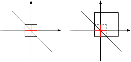
Figure 1: The sets $B_{2}^{f,\theta}(\mathbb{R})$ when $\mathcal{I}_{f,\theta}=[-1,1]$ (left plot) and $\mathcal{I}_{f,\theta}=[-1,3]$ (right plot). The red lines indicate the marginal projections.

Consequently, the coordinates of points on $B_{2}^{f,\theta}(\mathbb{R})$ and $B_{3}^{f,\theta}(\mathbb{R})$ cover the full image $(-1,1)$. Hence, $\mbox{MCSS}=2$.

Example 3.3.

Take $\varphi_{f}(\cdot;\theta)$ to be monotone on $S=\mathbb{R}$ with skewed image $(-1,3)$, say, independently of $\theta$. Then, while $B_{2}^{f,\theta}(\mathbb{R})$ and $B_{3}^{f,\theta}(\mathbb{R})$ remain defined as in Example 3.2 (with $(-1,3)$ replacing $(-1,1)$), coordinates of points in these domains do not cover the full image. In fact, in $B_{2}^{f,\theta}(\mathbb{R})$ these coordinates only cover the interval $(-1,1)$ (see Figure 1), in $B_{3}^{f,\theta}(\mathbb{R})$ these coordinates only cover the interval $(-1,2)$ and it is only from $n\geq 4$ onwards that the coordinates of points in $B_{n}^{f,\theta}(\mathbb{R})$ cover the full image. Hence, $\mbox{MCSS}=4$.

Example 3.4.

Take $f(x;\theta)=\theta\phi(\theta x)$ the Gaussian density with $\theta\in\mathbb{R}^{+}_{0}$ a scale parameter. We have $S=\mathbb{R}$, $\varphi_{\phi}(x;\theta)=\frac{1}{\theta}(1-\theta^{2}x^{2})$. Then $\varphi_{\phi}(\cdot;\theta)$ is invertible over $\mathbb{R}_{0}^{+}$ and $\mathbb{R}_{0}^{-}$, separately, and $\mathcal{I}_{f,\theta}(\mathbb{R}_{0}^{\pm})=(-\infty,1/\theta)$. Note that we have $\Pi_{x_{j}}(B_{n}^{f,\theta}(\mathbb{R}_{0}^{\pm}))=(-(n-1)/\theta,1/\theta)$ for all $j$, all $\theta$ and all $n\geq 2$. In other words, $B_{n}^{f,\theta}(\mathbb{R}_{0}^{\pm})$ is only asymptotically projectable. Hence, $\mbox{MCSS}=+\infty$.

Proof of Lemma 3.1 The assumptions on the image of $\varphi_{f}(\cdot;\theta)$ guarantee the existence of a point in $\mathcal{X}$ where $\varphi_{f}$ crosses the $x$-axis so that $B_{1}^{f,\theta}(\mathcal{X})=\{0\}$. Also, for all $n\geq 1$, we have $B_{n}^{f,\theta}(\mathcal{X})=H_{n}\cap(\mathcal{I}_{f,\theta}(\mathcal{X}))^{n}$; this follows by definition. Regarding the MCSS, first take $P^{-}_{f,\theta}=P^{+}_{f,\theta}=P$ (possibly infinite). Then, for all $n\geq 2$, $H_{n}\cap(-P,P)^{n}$ contains for each of the $n$ coordinates the full interval $(-P,P)$ (see Figure 1); hence $\mbox{MCSS}=2$. Next suppose that $P^{-}_{f,\theta}<P^{+}_{f,\theta}<\infty$ and consider a “worst-case scenario” by taking a point at the extreme of $H_{n}\cap(\mathcal{I}_{f,\theta}(\mathcal{X}))^{n}$, with one coordinate set to $b_{1}=P^{+}_{f,\theta}-\varepsilon$ for some $\varepsilon>0$. Then, in order to construct a sample satisfying $\sum_{i=1}^{n}b_{i}=0$, it is necessary to choose the remaining $n-1$-tuple $(b_{2},\ldots,b_{n})$ so as to satisfy $\sum_{i=2}^{n}b_{i}=-b_{1}$. Since the best choice in this respect consists in setting all $b_{i}$ near the other extremum $-P^{-}_{f,\theta}+\varepsilon^{\prime}$ for $\varepsilon^{\prime}>0$, we see that, depending on the magnitude of the ratio $P^{+}_{f,\theta}/P^{-}_{f,\theta}$, a given sample size $n$ may not be large enough for the equality to hold. In order to palliate this it suffices to take $N_{f,\theta}$ to be the smallest natural number such that $P^{+}_{f,\theta}-(N_{f,\theta}-1)P^{-}_{f,\theta}\leq 0$, that is, $N_{f,\theta}=\lceil{P^{+}_{f,\theta}}/{P^{-}_{f,\theta}}+1\rceil$. The case $P^{+}_{f,\theta}<P^{-}_{f,\theta}<\infty$ follows along the same lines, and hence

$$\mbox{MCSS}=\biggl{\lceil}\frac{\max(P^{+}_{f,\theta},P^{-}_{f,\theta})}{\min(P^{+}_{f,\theta},P^{-}_{f,\theta})}+1\biggr{\rceil}.$$

The same argumentation applies in the case where either one of $P^{+}_{f,\theta}$ or $P^{-}_{f,\theta}$ is infinite, this time with $\mbox{MCSS}=+\infty$. This concludes the proof.

Now look at the connection between the MCSS and MLE characterizations. Let $f$ and $g$ be two representatives of distinct e.c.’s with $f$ the target density. Under the assumption of $\theta$-differentiability of $g$, the defining equation (4) can be re-expressed as

$$\sum_{i=1}^{n}\varphi_{g}\bigl{(}x_{i};\hat{\theta}^{(n)}_{f}\bigl{(}\mathbf{x}^{(n)}\bigr{)}\bigr{)}=0\qquad\mbox{for all }\mathbf{x}^{(n)}\in S^{n},$$

which in turn can be rewritten as

$$\sum_{i=1}^{n}\varphi_{g}(x_{i};\theta)=0\qquad\mbox{for all }\theta\mbox{ and all }\mathbf{x}^{(n)}\mbox{ such that }\sum_{i=1}^{n}\varphi_{f}(x_{i};\theta)=0$$ (7)

(here $\theta$ and $\mathbf{x}^{(n)}$ are interdependent) or, equivalently,

$$\sum_{i=1}^{n}h(y_{i};\theta)=0\qquad\mbox{for all }\theta\mbox{ and all }\mathbf{y}^{(n)}\in B_{n}^{f,\theta}(\mathcal{X})$$ (8)

for each interval $\mathcal{X}$ on which $y\mapsto\varphi_{f}(y;\theta)$ is invertible for all $\theta$, with $h(y;\theta)=\varphi_{g}(\varphi_{f}^{-1}(y;\allowbreak\theta);\theta)$. Equation (8) completely identifies the function $h$ (and hence the interconnection between $g$ and $f$), at least when $B_{n}^{f,\theta}(\mathcal{X})$ is sufficiently rich. This richness depends strongly on the MCSS introduced in Lemma 3.1. Indeed supposing that (8) is only valid for a sample size smaller than the MCSS implies that portions of the images $\mathcal{I}_{f,\theta}(\mathcal{X})$ cannot be reached, so that $h$ cannot be identified over its entire support. This necessarily implies that $\mbox{MNSS}\geq\mbox{MCSS}$. It is, however, pointless to try to solve (8) in all generality and it is now necessary to specify the role of $\theta$ in order to pursue. We will do so in detail in the next sections, first in the case of location parameters; our arguments will afterwards adapt directly to other parameter choices.

4 MLE characterization for location parameter families

We start by identifying the e.c.’s for $\theta$ a location parameter. In such a case, $\Theta_{0}=S=\mathbb{R}$, and the location score functions are of the form $\varphi_{f}(x;\theta)=\varphi_{f}(x-\theta)=-f^{\prime}(x-\theta)/f(x-\theta)$ over $\mathbb{R}$, so that equation (3) turns into a simple first-order differential equation whose solution yields $g(x)=c(f(x))^{d}$ for some $d>0$ and $c$ the normalizing constant. Thus, all densities which are linked one to another via that relationship belong to a same e.c. We here attract the reader’s attention to the fact that, for $f=\phi$ the standard Gaussian density, such transformations reduce to a non-specification of the variance, which is clearly in line with Gauss’ MLE characterization as stated by Teicher [46] or Azzalini and Genton [4].

Our first main theorem is, in essence, a generalization of Gauss’ MLE characterization from the Gaussian distribution to the entire class of log-concave distributions with continuous score function.

Theorem 4.1.

Let $\mathcal{F}(\mathrm{loc})$ and $\mathcal{G}(\mathrm{loc})$ be two distinct location-based e.c.’s and let their respective representatives $f$ and $g$ be two continuously differentiable densities with full support $\mathbb{R}$. Let $x\mapsto\varphi_{f}(x)=-f^{\prime}(x)/f(x)$ be the location score function of $f$. If $\varphi_{f}$ is invertible over $\mathbb{R}$ and crosses the $x$-axis then there exists $N\in\mathbb{N}$ such that, for any $n\geq N$, we have $\hat{\theta}^{(n)}_{f}=\hat{\theta}^{(n)}_{g}$ for all samples of size $n$ if and only if there exist constants $c,d\in\mathbb{R}_{0}^{+}$ such that $g(x)=c(f(x))^{d}$ for all $x\in\mathbb{R}$, that is, if and only if $\mathcal{F}(\mathrm{loc})=\mathcal{G}(\mathrm{loc})$. The smallest integer for which this holds (the minimal necessary sample size) is $\mbox{MNSS}=\max\{N_{f},3\}$, with $N_{f}$ the MCSS as defined in Lemma 3.1.

Proof.

The sufficient condition is trivial. To prove necessity first note how our assumptions on $f$ ensure that the score function $\varphi_{f}$ is strictly increasing on the whole real line $\mathbb{R}$ and has a unique root. This allows us to write the image $\operatorname{Im}(\varphi_{f})$ as $(-P^{-}_{f},P^{+}_{f})$ with $0<P^{-}_{f},P^{+}_{f}\leq\infty$. The differentiability of $g$ and the nature of the parameter $\theta$ permit us to rewrite, for any admissible $\theta$, (7) as

$$\sum_{i=1}^{n}\varphi_{g}(x_{i}-\theta)=0\qquad\mbox{for all }\mathbf{x}^{(n)}\in\mathbb{R}^{n}\mbox{ such that }\sum_{i=1}^{n}\varphi_{f}(x_{i}-\theta)=0,$$ (9)

where $\varphi_{g}(x)=-g^{\prime}(x)/g(x)$. Using the strict monotonicity of $\varphi_{f}$ one then concludes that (9) is equivalent to requiring that $g$ satisfies

$$\sum_{i=1}^{n}h(b_{i})=0\qquad\mbox{for all }(b_{1},\ldots,b_{n})\in B_{n}^{f,\theta}(\mathbb{R}),$$ (10)

where $h=\varphi_{g}\circ\varphi_{f}^{-1}$ and $b_{i}=\varphi_{f}(x_{i}-\theta)$, $i=1,\ldots,n$, as in (5). In what follows, we shall use our liberty of choice among all $n$-tuples $\mathbf{b}^{(n)}\in B_{n}^{f,\theta}(\mathbb{R})$ in order to gain sufficient information on $h$ to conclude.

First, suppose that $P^{-}_{f,\theta}=P^{+}_{f,\theta}=P$, hence that the image of $\varphi_{f}$ is symmetric. We know from Lemma 3.1 that the corresponding MCSS equals 2, hence that two observations suffice to make $B_{n}^{f,\theta}(\mathbb{R})$ projectable. Therefore, for any $n\geq 2$, we can always build an $n$-tuple $b_{1},\ldots,b_{n}$ such that $b_{2}=-b_{1}$ for all $b_{1}\in(-P,P)$ and $b_{i}=0$ for $i=3,\ldots,n$. From (10) we then deduce that $h$ satisfies the equality $h(-a)=-h(a)$ for all $a\in(-P,P)$, hence that $h$ is odd on $(-P,P)$. Evidently this leaves $h$ undetermined, hence the MNSS must at least equal 3. For $n\geq 3$, choose an $n$-tuple such that $b_{3}=-b_{1}-b_{2}$ and $b_{i}=0$ for $i=4,\ldots,n$, for $b_{1},b_{2}\in(-P,P)$ such that $b_{1}+b_{2}\in(-P,P)$. Using (10) combined with the antisymmetry of $h$ we deduce that this function must satisfy

$$h(b)+h(c)=h(b+c)$$ (11)

for all $b,c\in(-P,P)$ such that $b+c\in(-P,P)$. One recognizes in (11) a (restricted) form of the celebrated Cauchy functional equation. Assume that $P<\infty$; then $h(P/2)$, say, is finite and standard arguments (see, e.g., Aczél and Dhombres [1]), imply that our solution $h$ satisfies $h(uP/2)=uh(P/2)$ for all $u\in(-2,2)$ and we conclude that $h(x)=dx$ for all $x\in(-P,P)$, with $d=h(P/2)/(P/2)\in\mathbb{R}$. Considering $x=\varphi_{f}(y)$ for $y\in\varphi_{f}^{-1}(-P,P)=\mathbb{R}$, we obtain that $\varphi_{g}(y)=d\varphi_{f}(y)$. Solving this first-order differential equation gives $g(y)=c(f(y))^{d}$ for all $y\in\mathbb{R}$, with $c$ a constant. In order for the function $g$ to be integrable over $\mathbb{R}$, the constant $d$ must be strictly positive; in order for $g$ to be positive and integrate to 1, the constant $c$ must be a normalizing constant. Thus, for $P<\infty$, the problem is solved. For $P=\infty$, the situation becomes even simpler as (11) is then precisely the Cauchy functional equation, and one may immediately draw the same conclusion as for finite $P$.

Let us now consider the case where $\varphi_{f}$ has a skewed image and set $P=\min(P^{-}_{f},P^{+}_{f})$ (note that $P$ is necessarily finite as otherwise $\operatorname{Im}(\varphi_{f})$ would be symmetric). First restricting our attention to $(-P,P)$, we can repeat the above arguments to deduce that $g(y)=c(f(y))^{d}$ for all $y\in\varphi_{f}^{-1}(-P,P)\subsetneq\mathbb{R}$. We thus further need to investigate the behavior of $h$ on the remaining part of $\operatorname{Im}(\varphi_{f})$ which, for the sake of simplicity, we denote as $\operatorname{Out}(P)$ (it is either $(-P^{-}_{f},-P)$ or $(P,P^{+}_{f})$). To this end, we precisely need to know the MCSS and hence call upon Lemma 3.1. Fixing $n\geq N_{f}$ and taking a sample $(b_{1},\ldots,b_{n})$ such that $\sum_{i=1}^{n}b_{i}=0$ with $b_{1}\in\operatorname{Out}(P)$ and $(b_{2},\ldots,b_{n})\in(-P,P)^{n-1}$, we can apply (10) to get $h(b_{1})+\sum_{i=2}^{n}h(b_{i})=0$ and hence, from our knowledge about the behavior of $h$ on $(-P,P)$, we deduce that

$$h(b_{1})=-\sum_{i=2}^{n}b_{i}h(P)/P=b_{1}h(P)/P,$$

since $h(P)$ is necessarily finite. Consequently we get $h(y)=yh(P)/P$ for all $y\in(-P,P)\cup\operatorname{Out}(P)=\operatorname{Im}(\varphi_{f})$ and $g(y)=c(f(y))^{d}$ for all $y\in\mathbb{R}$, and the conclusion follows.

The proof of the theorem is nearly complete: all that remains is to show that the $\mathrm{MNSS}=\max\{3,N_{f}\}$ is minimal and sufficient. The latter is immediate since if the result holds true for any sample of size $N=\mathrm{MNSS}$ then, for any larger sample size $M>\mathrm{MNSS}$, one can always consider $\mathbf{x}^{(M)}$ such that $\varphi_{f}(\mathbf{x}^{(M)})=\mathbf{b}^{(M)}\in B_{M}^{f,\theta}(\mathbb{R})$ is of the form $(b_{1},\ldots,b_{N},0,\ldots,0)$ and $(b_{1},\ldots,b_{N})\in B_{N}^{f,\theta}(\mathbb{R})$, and work as above to characterize the density. To prove the minimality of the $\mathrm{MNSS}$ it suffices to exhibit specific counter-examples. This is done in Examples 4.1 and 4.2 below. ∎

Example 4.1.

To see that $N=3$ is minimal when $\operatorname{Im}(\varphi_{f})$ is symmetric, we need to construct two distributions $g_{1}$, $g_{2}$ which share $f$’s MLE for all samples of size 2. Construct $g_{1}$ as in the proof of Theorem 4.1. To construct $g_{2}$, it suffices to replace the function $h$ from (10) with any odd function and to solve the resulting equation in $g$ (while ensuring integrability of $g$). If, for example, we choose $h(x)=dx^{3}$, then we readily obtain $g(y)=c\exp(-d\int_{-\infty}^{x}(\varphi_{f}(y))^{3}\,\mathrm{d}y)$; this is however not a density for all $f$, though a good choice for $f=\phi$ the Gaussian (for which $\varphi_{\phi}(x)=x$). Another way of proceeding is to work as in Azzalini and Genton [4] and to choose $h(y)=y+w^{\prime}(y)$ for some differentiable even function $w$.

Example 4.2.

Suppose that $\hat{\theta}^{(n)}_{f}=\hat{\theta}^{(n)}_{g}$ for all samples of size $n$ for some $n<N_{f}$ when $N_{f}>3$. Then, as is clear from Lemma 3.1, the whole domain (i.e., $\mathbb{R}$) of $f$ is not identified by our technique and it suffices to choose any density which is equal to $f$ on the maximal identifiable subdomain but differs elsewhere. Expressed in terms of $h$ for the case $P^{-}_{f}<P^{+}_{f}$, we can only identify $h$ on some interval $(-P^{-}_{f},P^{-}_{f}+a(n))$, say, with $0<a(n)<P^{+}_{f}-P^{-}_{f}$. On the remaining part $(P^{-}_{f}+a(n),P^{+}_{f})$, $h$ is undetermined and hence can take any possible form, implying that the relationship between $g$ and $f$ can only be established on the part $\varphi_{f}^{-1}(-P^{-}_{f},P^{-}_{f}+a(n))\subsetneq\mathbb{R}$.

As in Azzalini and Genton [4], it is sufficient to require in Theorem 4.1 that $g$ be continuously differentiable at a single point for everything to run smoothly. Pursuing in this vein, it is of course natural to enquire whether the result still holds if no such regularity assumption is imposed on $g$, that is, if we only suppose that the target density $f$ is differentiable but $g$ is a priori not. Put simply the question becomes that of enquiring whether the condition

$$\sum_{i=1}^{n}\log g\bigl{(}x_{i}-\hat{\theta}^{(n)}_{f}\bigl{(}\mathbf{x}^{(n)}\bigr{)}\bigr{)}\geq\sum_{i=1}^{n}\log g(x_{i}-\theta)$$ (12)

for all $\mathbf{x}^{(n)}\in\mathbb{R}^{n}$ and all $\theta\in\mathbb{R}$ suffices to determine $g$. This is the approach adopted, for example, in Teicher [46], Kagan, Linnik and Rao [27] or Marshall and Olkin [34], where it is shown that having the likelihood condition (12) with $\hat{\theta}^{(n)}_{f}$ the sample mean implies $g$ is the Gaussian as soon as the result holds for all samples of sizes 2 and 3 simultaneously. Interestingly, in our framework, this arguably more general assumption on $g$ comes with a cost: our method of proof then necessitates imposing more restrictive assumptions on $f$ and requiring the likelihood equations to hold for two sample sizes simultaneously.

Theorem 4.2.

Let $\mathcal{F}(\mathrm{loc})$ and $\mathcal{G}(\mathrm{loc})$ be two distinct location-based e.c.’s and let their respective representatives $f$ and $g$ be two continuous densities with full support $\mathbb{R}$. Suppose that $f$ is symmetric and continuously differentiable, and assume that its location score function $\varphi_{f}(x)$ is invertible over $\mathbb{R}$ and crosses the $x$-axis. Then we have $\hat{\theta}^{(n)}_{f}=\hat{\theta}^{(n)}_{g}$ for all samples of sizes 2 and $n\geq 3$ simultaneously if and only if there exist constants $c,d\in\mathbb{R}_{0}^{+}$ such that $g(x)=c(f(x))^{d}$ for all $x\in\mathbb{R}$, that is, if and only if $\mathcal{F}(\mathrm{loc})=\mathcal{G}(\mathrm{loc})$.

Proof.

Our proof, which extends that of Teicher [46] from the Gaussian case to the entire class of symmetric log-concave densities $f$, proceeds in two main steps: we first show that our assumptions on $g$ in fact entail that $g$ is continuously differentiable, and then conclude by applying Theorem 4.1. The additional sample size $n=2$ needed here stems from the first step.

Condition (12) can be rewritten as

$$\sum_{i=1}^{n}\log g(y_{i})\geq\sum_{i=1}^{n}\log g(y_{i}-\theta)$$

for all $\theta\in\mathbb{R}$ and $y_{1},\ldots,y_{n}$ satisfying $\sum_{i=1}^{n}\varphi_{f}(y_{i})=0$. The latter expression in turn is equivalent to

$$\sum_{i=1}^{n-1}\log g(y_{i})+\log g\Biggl{(}\varphi_{f}^{-1}\Biggl{(}-\sum_{j=1}^{n-1}\varphi_{f}(y_{j})\Biggr{)}\Biggr{)}$$

(13)

$$\quad\geq\sum_{i=1}^{n-1}\log g(y_{i}-\theta)+\log g\Biggl{(}\varphi_{f}^{-1}\Biggl{(}-\sum_{j=1}^{n-1}\varphi_{f}(y_{j})\Biggr{)}-\theta\Biggr{)}.$$

Arguing as in Teicher [46], it is sensible to confine our attention at first to symmetric densities $g$. Using the assumed symmetric nature of $f$ (and hence the oddness of $\varphi_{f}^{-1}$), considering the sample size $n=2$ and setting observation $y_{1}$ equal to some $y\in\mathbb{R}$, (4) simplifies into

$$2\log g(y)\geq\log g(y-\theta)+\log g(y+\theta)$$ (14)

for all $y,\theta\in\mathbb{R}$. Since $\log g$ is everywhere finite, concave according to (14), and inherits measurability from $g$, it is an a.e.-continuously differentiable function. Arrived at this point, we may apply Theorem 4.1 to conclude (note that the oddness of $\varphi_{f}$ makes Theorem 4.1 hold with MNSS equal to $3$).

Finally, for non-necessarily symmetric densities $g$, we can follow exactly the argumentation from Teicher [46] and derive that the previously obtained solution is the only one, hence the claim holds. ∎

We stress the fact that, as in Teicher [46], we may further weaken our assumptions on $g$ by only requiring that it is lower semi-continuous at the origin and need not have full support $\mathbb{R}$. Indeed, as shown in Teicher’s proof, continuity and a.e.-positivity ensue from the above arguments.

One may wonder whether the symmetry assumption on the target density $f$ is necessary or whether this second general location MLE characterization theorem may in fact hold for the entire class of log-concave densities as well. Our method of proof indeed requires this assumption so as to enable us to deal with such quantities as $\varphi_{f}^{-1}(-\sum_{j=1}^{n-1}\varphi_{f}(y_{j}))$ in (4); without any assumption on $f$, for $n=2$, this expression does not simplify into the agreeable form $-y_{1}$. Similarly, one may wonder whether it is necessary to suppose the result to hold for two sample sizes simultaneously or whether one single sample size $N\geq 3$ might not suffice. We leave as open problems the question whether these assumptions are necessary or simply sufficient.

Finally, our Theorems 4.1 and 4.2 do not cover target densities whose location score function is monotone but not invertible over the entire real line, that is, piecewise constant. We do not consider explicitly such setups here since they do not assure that the MLE is defined in a unique way. The strategy we however suggest consists in applying our results on the monotonicity intervals, to draw the necessary conclusions and express $g$ in terms of $f$ on those intervals. If we add the condition of monotonicity of $\varphi_{g}$, the equality $\varphi_{g}(x)=d\varphi_{f}(x)$ has to hold over the entire support $\mathbb{R}$ as monotonicity imposes $\varphi_{g}$ to be constant outside the above-mentioned intervals. Since we here do not implicitly use the intervals where $\varphi_{f}$ is constant, there might exist better strategies, and consequently the smallest possible sample size we obtain by following this scheme is an upper bound for the true MNSS. The most extreme situation takes place when the target is a Laplace distribution, in which case $\varphi_{f}(x)=\operatorname{sign}(x)$; we refer to Kagan, Linnik and Rao [27] for a treatment of this particular distribution. We will return to these matters briefly in Section 8.

5 MLE characterization for scale parameter families

As for location parameter families, we start by identifying the e.c.’s when $\theta$ plays the role of a scale parameter. In such a setup, $\Theta_{0}=\mathbb{R}_{0}^{+}$, $S=\mathbb{R}$, $\mathbb{R}^{+}_{0}$ or $\mathbb{R}^{-}_{0}$ in view of assumption (A2), and the scale score functions are of the form $\varphi_{f}(x;\theta)=\frac{1}{\theta}\psi_{f}(\theta x):=\frac{1}{\theta}(1+\theta xf^{\prime}(\theta x)/f(\theta x))$ over $S$, so that equation (3) turns into another quite simple first-order differential equation whose solution leads to $g(x)=c|x|^{d-1}(f(x))^{d}$ for some $d>0$ (such that $g$ is integrable) and $c$ the normalizing constant. This relationship defines the scale-based e.c.’s. It is to be noted that $c=d=1$ when the origin belongs to the support, that is, when $S=\mathbb{R}$, in which case the e.c.’s reduce to singletons $\{f\}$.

Our main scale MLE characterization theorem is the exact equivalent of Theorem 4.1 with $\psi_{f}$ replacing $\varphi_{f}$, hence its proof is omitted.

Theorem 5.1.

Let $\mathcal{F}(\mathrm{sca})$ and $\mathcal{G}(\mathrm{sca})$ be two distinct scale-based e.c.’s and let their respective representatives $f$ and $g$ be two continuously differentiable densities with common support $S$ (either $\mathbb{R},\mathbb{R}_{0}^{+}$ or $\mathbb{R}_{0}^{-}$). Let $\psi_{f}(x)=1+xf^{\prime}(x)/f(x)$ be the scale score function of $f$. If $\psi_{f}$ is invertible over $S$ and crosses the $x$-axis then there exists $N\in\mathbb{N}$ such that, for any $n\geq N$, we have $\hat{\theta}^{(n)}_{f}=\hat{\theta}^{(n)}_{g}$ for all samples of size $n$ if and only if there exist constants $c,d\in\mathbb{R}_{0}^{+}$ such that $g(x)=c|x|^{d-1}(f(x))^{d}$ for all $x\in S$ (with $c=d=1$ for $S=\mathbb{R}$), that is, if and only if $\mathcal{F}(\mathrm{sca})=\mathcal{G}(\mathrm{sca})$. The smallest integer for which this holds is $\mbox{MNSS}=\max\{N_{f},3\}$, with $N_{f}$ the MCSS as defined in Lemma 3.1.

As in the case of a location parameter, requiring differentiability of the $g$’s is not indispensable. One could indeed restrict the class of target distributions under consideration, as in Teicher [46]. We leave this as an easy exercise.

When dealing with scale families it is natural to work as in Teicher [46] and add a scale-identification condition of the form

$$\lim_{x\rightarrow 0}{g(\lambda x)}/{g(x)}=\lim_{x\rightarrow 0}{f(\lambda x)}/{f(x)}\qquad\forall\lambda>0.$$ (15)

Imposing this condition in Theorem 5.1 allows, at least when the limit is finite, positive and does not equal $1/\lambda$ (which occurs only for pathological cases; we leave as an exercise to the reader to see why this type of limiting behavior precludes identifications), to deduce that $c=d=1$ for $S=\mathbb{R}_{0}^{+}$ and $\mathbb{R}_{0}^{-}$, and hence $g=f$ in all cases. Interestingly Teicher already remarks that this “seemingly ad hoc condition appears to be crucial”; this is clearly the case for a complete identification of the family of densities which share a scale MLE.

The invertibility condition imposed on $\psi_{f}$ is as natural in a scale family context as the invertibility condition on $\varphi_{f}$ in a location family setup (see Lehmann and Casella [30], page 502). Unfortunately it suffers from one major drawback for $S=\mathbb{R}$: requiring invertibility of $\psi_{f}$ over the whole real line forces us to discard several interesting cases such as, for example, the standard normal density $\phi$, for which $\psi_{\phi}(x)=1-x^{2}$ is only invertible over the positive and negative real half-lines, respectively. More generally any symmetric density $f$ for which $\varphi_{f}$ is invertible over $\mathbb{R}$ will suffer from that same problem and hence will not be characterizable by means of Theorem 5.1. This flaw is nevertheless easily fixed, since Lemma 3.1 is applicable even if $\psi_{f}$ is only invertible over portions of its support. This leads to our next general result (whose proof is omitted).

Theorem 5.2.

Let $\mathcal{F}(\mathrm{sca})$ and $\mathcal{G}(\mathrm{sca})$ be two distinct scale-based e.c.’s and let their respective representatives $f$ and $g$ be two continuously differentiable densities with full support $\mathbb{R}$. Let the scale score function $\psi_{f}(x)=1+xf^{\prime}(x)/f(x)$ be invertible and cross the $x$-axis over $\mathbb{R}_{0}^{+}$ and $\mathbb{R}_{0}^{-}$, respectively. Then there exists $N\in\mathbb{N}$ such that, for any $n\geq N$, we have $\hat{\theta}^{(n)}_{f}=\hat{\theta}^{(n)}_{g}$ for all samples of size $n$ if and only if $g(x)=f(x)$ for all $x\in\mathbb{R}$. Moreover the MNSS is given by $\max\{\mbox{MNSS}_{-},\mbox{MNSS}_{+}\}$, where $\mbox{MNSS}_{-}$ and $\mbox{MNSS}_{+}$, respectively, stand for the MNSS required on each half-line.

It should be noted that the scale condition (15) is not necessary here since we are working on the entire support $S=\mathbb{R}$ which imposes that $d=1$ as otherwise the non-vanishing density $g$ would vanish at 0.

Finally note that the separation of the two real half-lines is tailored for scale families because both $\mathbb{R}_{0}^{+}$ and $\mathbb{R}_{0}^{-}$ are invariant under the action of the scale parameter, which permits us to work on each half-line separately and put the ends together by continuity. The same would not hold true for location families due to a lack of invariance, that is, we could not “glue together” location characterizations valid on complementary subsets of the support.

6 MLE characterization for one-parameter group families

The relevance of our approach is not confined to location and scale families, but can be used for other $\theta$-parameter families with $\theta$ neither a location nor a scale parameter. In this section, we shall consider general one-parameter group families and provide them with MLE characterization results. Group families play a central role in statistics as they contain several well-known parametric families (location, scale, several types of skew distributions as shown in Ley and Paindaveine [31]$,\ldots$) and allow for significant simplifications of the data under investigation (see Lehmann and Casella [30], Section 1.4, for more details). To the best of the authors’ knowledge, there exist no MLE characterizations for group families other than the location and scale families.

A univariate group family of distributions is obtained by subjecting a scalar random variable with a fixed distribution to a suitable family of transformations. More prosaically, let $X$ be a random variable with density $f$ defined on its support $S$ and consider a transformation group $\mathcal{H}$ (meaning that it is closed under both composition and inversion) of monotone increasing functions $H_{\theta}\mathchoice{\nobreak\,\colon}{\nobreak\,\colon}{\nobreak\,\colon\;}{\nobreak\,\colon\;}D\subseteq\mathbb{R}\rightarrow S$ depending on a single real parameter $\theta\in\Theta_{0}$. The family of random variables $\{H_{\theta}^{-1}(X),H_{\theta}\in\mathcal{H}\}$ is called a group family. These variables possess densities of the form

$$f_{\mathcal{H}}(x;\theta):=H_{\theta}^{\prime}(x)f\bigl{(}H_{\theta}(x)\bigr{)},$$ (16)

where $H_{\theta}^{\prime}$ stands for the derivative of the mapping $x\mapsto H_{\theta}(x)$ (which we therefore also suppose everywhere differentiable); their support $D$ does not depend on $\theta$. We call $\theta$ a $\mathcal{H}$-parameter for $f(x;\theta)$. The most prominent examples are of course $\mathcal{H}_{\mathrm{loc}}:=\{H_{\theta}(x)=x-\theta,x,\theta\in\mathbb{R}\}$, leading to location families, and $\mathcal{H}_{\mathrm{sca}}:=\{H_{\theta}(x)=\theta x,x\in S,\theta\in\mathbb{R}_{0}^{+}\}$ for $S=\mathbb{R},\mathbb{R}_{0}^{+}$ and $\mathbb{R}_{0}^{-}$, yielding scale families. For further examples, we refer to Lehmann and Casella [30], Section 1.4, and the references therein.

Let us now determine the e.c.’s for $\mathcal{H}$-parameter families. Assuming that the mappings $\theta\mapsto H_{\theta}(x)$ and $\theta\mapsto H_{\theta}^{\prime}(x)$ are differentiable, the $\mathcal{H}$-score function associated with densities of the form (16) corresponds to

$$\varphi_{f}^{\mathcal{H}}(x;\theta):=\frac{\partial_{\theta}H_{\theta}^{\prime}(x)}{H_{\theta}^{\prime}(x)}+\frac{\partial_{\theta}H_{\theta}(x)f^{\prime}(H_{\theta}(x))}{f(H_{\theta}(x))}$$ (17)

over $D$ (it is set to 0 outside $D$). Extracting e.c.’s from equation (3) is all but evident here, as (i) there is no structural reason for $\partial_{\theta}H_{\theta}(x)$ to cross the $x$-axis so as to allow to fix $d$ to 1 as in the scale case over $\mathbb{R}$, and (ii) the generality of the model hampers a clear understanding of the role of $\theta$ inside the densities. Especially the latter point is crucial, as e.c.’s cannot depend on the parameter. We thus need to further specify the form of $f_{\mathcal{H}}(x;\theta)$ or, more exactly, the form of the transformations in $\mathcal{H}$ and thus the action of $\theta$ inside the densities. We choose to restrict our attention to transformations $H_{\theta}$ satisfying the following two factorizations:

$$\cases{\partial_{\theta}H_{\theta}(x)=T(\theta)U_{1}\bigl{(}H_{\theta}(x)\bigr{)},\vspace*{2pt}\cr\displaystyle\frac{\partial_{\theta}H_{\theta}^{\prime}(x)}{H_{\theta}^{\prime}(x)}=T(\theta)U_{2}\bigl{(}H_{\theta}(x)\bigr{)},}$$

where $T$, $U_{1}$ and $U_{2}$ are real-valued functions. At first sight, such restrictions might seem severe, but there exist numerous one-parameter transformations enjoying these factorizations, including:

• transformations of the form $H_{\theta}(x)=a_{1}(x)+a_{2}(\theta)$ defined over the entire real line, with $a_{1}$ a monotone increasing differentiable function over $\mathbb{R}$ and $a_{2}$ any real-valued differentiable function. These transformations lead to “generalized location families” and satisfy the above factorizations with $T(\theta)=a_{2}^{\prime}(\theta)$, $U_{1}(x)=1$ and $U_{2}(x)=0$;

• transformations of the form $H_{\theta}(x)=a_{1}(x)a_{2}(\theta)$ defined over $\mathbb{R},\mathbb{R}_{0}^{+}$ or $\mathbb{R}_{0}^{-}$, with $a_{1}$ a monotone increasing differentiable function over the corresponding domain and $a_{2}$ a positive real-valued differentiable function. These transformations lead to “generalized scale families” and satisfy the above factorizations with $T(\theta)=a_{2}^{\prime}(\theta)/a_{2}(\theta)$, $U_{1}(x)=x$ and $U_{2}(x)=1$;

• transformations of the form $H_{\theta}(x)=\operatorname{sinh}(\operatorname{arcsinh}(x)+\theta)$ defined over $\mathbb{R}$. These are the so-called sinh–arcsinh transformations put to use in Jones and Pewsey [26] in order to define sinh–arcsinh distributions which allow to cope for both skewness and kurtosis. The above factorizations are verified for $T(\theta)=1$, $U_{1}(x)=\sqrt{1+x^{2}}$ and $U_{2}(x)=x/\sqrt{1+x^{2}}$.

Under these premisses, equation (3) becomes

$$d\biggl{(}U_{2}\bigl{(}H_{\theta}(x)\bigr{)}+U_{1}\bigl{(}H_{\theta}(x)\bigr{)}\frac{f^{\prime}(H_{\theta}(x))}{f(H_{\theta}(x))}\biggr{)}$$

$$\quad=U_{2}\bigl{(}H_{\theta}(x)\bigr{)}+U_{1}\bigl{(}H_{\theta}(x)\bigr{)}\frac{g^{\prime}(H_{\theta}(x))}{g(H_{\theta}(x))}\qquad\forall x\in D,$$

which can be rewritten as

$$d\biggl{(}U_{2}(x)+U_{1}(x)\frac{f^{\prime}(x)}{f(x)}\biggr{)}=U_{2}(x)+U_{1}(x)\frac{g^{\prime}(x)}{g(x)}\qquad\forall x\in S.$$

This first-order differentiable equation admits as solution $g(x)=c\exp((d-1)\int^{x}U_{2}(y)/\allowbreak U_{1}(y)\,\mathrm{d}y)(f(x))^{d}$ for some $d>0$ (such that $g$ is integrable) and $c$ a normalizing constant. This relationship establishes the $\mathcal{H}$-based e.c.’s. As for the scale case, $c=d=1$ when there exists $x_{0}\in S$ such that $U_{1}(x_{0})=0$, yielding e.c.’s constituted of singletons $\{f\}$.

For each transformation group $\mathcal{H}$, we obtain the following MLE characterization theorem for one-parameter group families. The proof of this result contains nothing new and is thus omitted.

Theorem 6.1.

Let $\mathcal{F}(\mathcal{H})$ and $\mathcal{G}(\mathcal{H})$ be two distinct $\mathcal{H}$-based e.c.’s and let their respective representatives $f$ and $g$ be two continuously differentiable densities with common full support $S$. Let $\varphi_{f}^{\mathcal{H}}:=U_{2}(x)+U_{1}(x)f^{\prime}(x)/f(x)$ be the $\mathcal{H}$-score function of $f$. If $\varphi_{f}^{\mathcal{H}}$ is invertible over $S$ then there exists $N\in\mathbb{N}$ such that, for any $n\geq N$, we have $\hat{\theta}^{(n)}_{f}=\hat{\theta}^{(n)}_{g}$ for all samples of size $n$ if and only if there exist constants $c,d\in\mathbb{R}_{0}^{+}$ such that $g(x)=c\exp((d-1)\int^{x}U_{2}(y)/U_{1}(y)\,\mathrm{d}y)(f(x))^{d}$ for all $x\in S$ (with $c=d=1$ if there exists $x_{0}\in S$ such that $U_{1}(x_{0})=0$), that is, if and only if $\mathcal{F}(\mathcal{H})=\mathcal{G}(\mathcal{H})$. The smallest integer for which this holds is $\mbox{MNSS}=\max\{N_{f},3\}$, with $N_{f}$ the MCSS as defined in Lemma 3.1.

Aside from location- and scale-based characterizations (or variations thereof) which are already available from Theorems 4.1 and 5.1, Theorem 6.1 allows, inter alia, to characterize asymmetric distributions (namely the sinh–arcsinh distributions of Jones and Pewsey [26]) with respect to their skewness parameter.

7 Examples

In this section, we analyze and discuss several examples of absolutely continuous distributions in light of the findings of the previous sections. We indicate, in each case, the corresponding MNSS. As we shall see, we hereby retrieve a wide variety of existing results, and obtain several new ones. We stress that, in each case discussed below, the minimal sample size provided is optimal in the sense that counter-examples can be constructed if the results only are supposed to hold true for smaller sample sizes. Moreover, we attract the reader’s attention to the fact that, in some examples of scale-based characterizations, we need the scale-identification condition (15), whereas in others it is superfluous, as explained in Section 5.

For the sake of clarity, we will adopt in this section the commonly used notations $\hat{\mu}^{(n)}_{f}$ and $\hat{\sigma}^{(n)}_{f}$ for location and scale ML estimators.

7.1 The Gaussian distribution

Consider the Gaussian distribution whose MLE characterizations for both the location and the scale parameter have been extensively discussed in the literature. For $\phi$ the standard Gaussian density, we get $\varphi_{\phi}(x)=x$ which is invertible over $\mathbb{R}$ and has image $\operatorname{Im}(\varphi_{\phi})=\mathbb{R}$. As already mentioned several times, the MLE $\hat{\mu}^{(n)}_{\phi}$ is given by the sample arithmetic mean $\bar{x}$. Thus, Theorems 4.1 and 4.2 apply, with $\mbox{MNSS}=3$ since $P^{+}_{\phi}=P^{-}_{\phi}=\infty$. The first corresponds to Azzalini and Genton [4], Theorem 1, the second to Teicher [46], Theorem 1. Regarding the scale characterization for $\hat{\sigma}^{(n)}_{\phi}=(n^{-1}\sum_{i=1}^{n}x_{i}^{2})^{1/2}$, direct calculations reveal that $\psi_{\phi}(x)=1-x^{2}$ which is invertible over both $\mathbb{R}^{+}_{0}$ and $\mathbb{R}^{-}_{0}$ and maps both domains onto $(-\infty,1)$. The conditions of Theorem 5.2 are thus fulfilled and yield that the MNSS equals $\infty$. Hence we retrieve Teicher [46], Theorem 3.

7.2 The gamma distribution

Consider the gamma distribution with tail parameter $\alpha>0$, whose density is given by

$$f(x)=\frac{1}{\Gamma(\alpha)}x^{\alpha-1}\exp(-x)\mathbb{I}_{(0,\infty)}(x),$$

where $\mathbb{I}_{A}$ represents the indicator function of the set $A$. The exponential density is a special case of gamma densities obtained by setting $\alpha=1$. Gamma distributions are not natural location families; this can be seen, for instance, by considering the exponential case, where $\varphi_{f}(x)=1$ and hence the location likelihood equations make no sense. Within the framework of the current paper, we anyway do not provide a location-based MLE characterization of gamma densities, since their support is only $\mathbb{R}_{0}^{+}$ instead of $\mathbb{R}$. On the contrary, gamma densities allow for agreeable scale characterizations. Indeed easy computations show that $\varphi_{f}(x)=(-\alpha+1)/{x}+1$, $\psi_{f}(x)=\alpha-x$, which is thus invertible over $\mathbb{R}_{0}^{+}$, $\operatorname{Im}(\psi_{f})=(-\infty,\alpha)$ and $\hat{\sigma}^{(n)}_{f}=\alpha^{-1}\bar{x}$. We can therefore use Theorem 5.1 in combination with the scale-identification condition (15) to obtain that the gamma distribution with shape $\alpha$ is characterizable w.r.t. its scale MLE $\alpha^{-1}\bar{x}$ for an infinite MNSS. We hereby recover Teicher [46], Theorem 2, and the univariate case of Marshall and Olkin [34], Theorem 5.1.

7.3 The generalized Gaussian distribution

Consider the one-parameter generalization of the normal distribution proposed in Ferguson [17], with density

$$f(x)=\frac{|\gamma|\alpha^{\alpha}}{\Gamma(\alpha)}\exp\bigl{(}\alpha\gamma x-\alpha\exp(\gamma x)\bigr{)},$$

where $\alpha>0$ and $\gamma$, the additional parameter, differs from zero (Ferguson has proved that, for $\gamma\rightarrow 0$, this density converges to the Gaussian). This probability law is in fact strongly related to the gamma distribution, as it is defined as $\gamma^{-1}\log(X)$ with $X\sim\operatorname{Gamma}(\alpha)$. Now, direct calculations yield $\varphi_{f}(x)=-\alpha\gamma(1-\exp(\gamma x))$, invertible over $\mathbb{R}$, $\operatorname{Im}(\varphi_{f})=\operatorname{sign}(\gamma)(-\alpha|\gamma|,\infty)$ and $\hat{\mu}^{(n)}_{f}=\gamma^{-1}\log(n^{-1}\sum_{i=1}^{n}\exp(\gamma x_{i}))$. Hence, from Theorem 4.1, we deduce that these distributions can be characterized in terms of their location parameter, with MNSS equal to $\infty$; we retrieve Ferguson [17], Theorem 5. Concerning the scale part, $\psi_{f}(x)=\alpha\gamma x(1-\exp(\gamma x))+1$ is not invertible over the whole real line, but invertible over both $\mathbb{R}^{+}_{0}$ and $\mathbb{R}^{-}_{0}$, and maps both half-lines onto $(-\infty,1)$. Consequently, Theorem 5.2 reveals that this distribution admits as well a scale MLE characterization result, with infinite MNSS.

7.4 The Laplace distribution

Consider the Laplace distribution with density

$$f(x)=\exp\bigl{(}-|x|\bigr{)}/2.$$

One easily obtains $\varphi_{f}(x)=\operatorname{sign}(x)$ and $\psi_{f}(x)=-x\operatorname{sign}(x)+1$. While the former function is clearly not invertible at all (but allows for a location MLE characterization; see the end of Section 5), the latter is invertible on both $\mathbb{R}_{0}^{-}$ and $\mathbb{R}_{0}^{+}$ with $\operatorname{Im}(\psi_{f})=(-\infty,1)$. Hence Theorem 5.2 applies and reveals that the Laplace distribution is also MLE-characterizable w.r.t. its scale parameter (with infinite MNSS), which complements the existing results on MLE characterizations of the Laplace distribution from Ghosh and Rao [21], Kagan, Linnik and Rao [27], Marshall and Olkin [34].

Corollary 7.1.

The statistic

$$\hat{\sigma}^{(n)}_{f}=\Biggl{(}n^{-1}\sum_{i=1}^{n}|x_{i}|\Biggr{)}^{-1}$$

is the MLE of the scale parameter $\sigma$ within scale families over $\mathbb{R}$ for all samples of all sample sizes if and only if the samples are drawn from a Laplace distribution.

For the sake of readability we will, here and in the sequel, content ourselves with such informal statements of our characterization results; rigorous statements are straightforward adaptations of the corresponding theorems from the previous sections.

7.5 The Weibull distribution

Consider the Weibull distribution with density

$$f(x)=kx^{k-1}\exp\bigl{(}-x^{k}\bigr{)}\mathbb{I}_{(0,\infty)}(x),$$

where $k>0$ is the shape parameter. As for gamma distributions, we do not provide a location-based MLE characterization for this distribution on the positive real half-line. Regarding the scale part, we have $\varphi_{f}(x)=-\frac{k-1}{x}+kx^{k-1}$, $\psi_{f}(x)=k(1-x^{k})$, clearly invertible over $\mathbb{R}_{0}^{+}$, and $\operatorname{Im}(\psi_{f})=(-\infty,k)$. Thus, all conditions for Theorem 5.1 are satisfied, from which we derive, under the scale-identification condition (15), the following, to the best of our knowledge new, MLE characterization of the Weibull distribution.

Corollary 7.2.

Let condition (15) hold. Then the statistic

$$\hat{\sigma}^{(n)}_{f}=\Biggl{(}n^{-1}\sum_{i=1}^{n}x_{i}^{k}\Biggr{)}^{-1/k}$$

is the MLE of the scale parameter $\sigma$ within scale families over $\mathbb{R}_{0}^{+}$ for all samples of all sample sizes if and only if the samples are drawn from a Weibull distribution with shape parameter $k$.

7.6 The Gumbel distribution

Consider the Gumbel distribution with density

$$f(x)=\exp\bigl{(}-x-\exp(-x)\bigr{)}.$$

Straightforward manipulations yield $\varphi_{f}(x)=1-\exp(-x)$, invertible over $\mathbb{R}$ and $\operatorname{Im}(\varphi_{f})=(-\infty,1)$. Thus, all conditions for Theorem 4.1 are satisfied, from which we derive the following, to the best of our knowledge new, MLE characterization of the Gumbel distribution (actually, of the power-Gumbel distribution).

Corollary 7.3.

The statistic

$$\hat{\mu}^{(n)}_{f}=\log\Biggl{[}\Biggl{(}n^{-1}\sum_{i=1}^{n}\exp(-x_{i})\Biggr{)}^{-1}\Biggr{]}$$

is the MLE of the location parameter $\mu$ within location families over $\mathbb{R}$ for all samples of all sample sizes if and only if the samples are drawn from a power-Gumbel distribution with density $c\exp(-dx-d\exp(-x))$ for $c,d\in\mathbb{R}_{0}^{+}$.

As for the scale part, it follows that $\psi_{f}(x)=x(-1+\exp(-x))+1$, non-invertible over $\mathbb{R}$ but invertible over both $\mathbb{R}_{0}^{+}$ and $\mathbb{R}_{0}^{-}$, and $\operatorname{Im}(\psi_{f})=(-\infty,1)$. Consequently, Theorem 5.2 applies and shows that the Gumbel distribution (here not a general power-Gumbel distribution) allows as well for a MLE characterization with respect to its scale parameter (with corresponding MNSS equal to $\infty$).

7.7 The Student distribution

Consider the Student distribution with $\nu>0$ degrees of freedom, with density

$$f(x)=\kappa(\nu)\biggl{(}1+\frac{x^{2}}{\nu}\biggr{)}^{-(\nu+1)/2}$$

for $\kappa(\nu)$ the appropriate normalizing constant. Then although the support of $f$ is the whole real line, the location score function $\varphi_{f}(x)=(\nu+1)\frac{x}{\nu+x^{2}}$ is not invertible and thus we cannot provide a location characterization. On the other hand straightforward computations yield

$$\psi_{f}(x)=1-(\nu+1)\frac{x^{2}}{\nu+x^{2}}=-\nu+\frac{\nu(\nu+1)}{\nu+x^{2}}.$$

This function is invertible over both the positive and the negative real half-line with $\operatorname{Im}(\psi_{f})=(-\nu,1)$ and thus the Student distribution with $\nu$ degrees of freedom is by virtue of Theorem 5.2 scale-characterizable with

$$\mathrm{MNSS}=\cases{\displaystyle\biggl{\lceil}1+\frac{1}{\nu}\biggr{\rceil},&\quad if $\nu<1$,\vspace*{2pt}\cr 3,&\quad if $\nu=1$,\vspace*{2pt}\cr\lceil 1+\nu\rceil,&\quad if $\nu>1$.}$$

This result generalizes the scale characterization of the Gaussian distribution, which is a particular case of the Student distributions when $\nu$ tends to infinity. Note that the expression above then indeed yields an infinite MNSS. Moreover, the Cauchy distribution, obtained for $\nu=1$, is MLE-characterizable w.r.t. its scale parameter with an MNSS of 3.

7.8 The logistic distribution

Consider the logistic distribution, whose density is given by

$$f(x)=\frac{\mathrm{e}^{-x}}{(1+\mathrm{e}^{-x})^{2}}.$$

Straightforward manipulations yield $\varphi_{f}(x)=\tanh(x/2)$, which is invertible over $\mathbb{R}$ and $\operatorname{Im}(\varphi_{f})=(-1,1)$. Theorem 4.1 applies and yields the (to the best of our knowledge) first MLE characterization of the (power-)logistic distribution with respect to its location parameter (with corresponding MNSS equal to $3$).

Further, $\psi_{f}(x)=1-x\tanh(x/2)$ is not invertible over the whole real line, but is invertible over both $\mathbb{R}_{0}^{+}$ and $\mathbb{R}_{0}^{-}$, and maps both half-lines onto $(-\infty,1)$. Consequently, Theorem 5.2 applies and yields the (to the best of our knowledge) first scale MLE characterization of the logistic distribution, with infinite MNSS.

7.9 The sinh–arcsinh skew-normal distribution

As a final example, we consider the sinh–arcsinh skew-normal distribution of Jones and Pewsey [26] whose density is given by

$$f(x)=\frac{1}{\sqrt{2\uppi}}\frac{(1+\operatorname{sinh}^{2}(\operatorname{arcsinh}(x)+\delta))^{1/2}}{(1+x^{2})^{1/2}}\mathrm{e}^{-\operatorname{sinh}^{2}(\operatorname{arcsinh}(x)+\delta)/2},$$

where $\delta\in\mathbb{R}$ is a skewness parameter regulating the asymmetric nature of the distribution. Clearly, for $\delta=0$, corresponding to the symmetric situation, one retrieves the standard normal distribution. Now, straightforward but tedious calculations provide us with expressions for $\varphi_{f}$ and $\psi_{f}$ which can both be seen to be non-invertible. Hence, no location-based nor scale-based characterizations can be obtained. However, the sinh–arcsinh skew-normal distribution can be characterized w.r.t. its skewness parameter. As shown in Section 6, the sinh–arcsinh transform belongs to the class of transforms leading to group families. Consequently, its skewness score function is given by

$$\varphi_{f}^{\mathcal{H}}(x)=U_{2}(x)+U_{1}(x)\frac{\phi^{\prime}(x)}{\phi(x)}=\frac{-x^{3}}{(1+x^{2})^{1/2}}$$

with $\phi$ the standard Gaussian density. This mapping is invertible over $\mathbb{R}$ with symmetric image $\mathbb{R}$. Theorem 6.1 therefore applies and yields the (to the best of our knowledge) first MLE characterization of the sinh–arcsinh skew-normal distribution (with respect to its skewness parameter) with an MNSS equal to 3.

8 Discussion and open problems

In this article, we have provided a unified treatment of the topic of MLE characterizations for one-parameter group families of absolutely continuous distributions satisfying certain regularity conditions. A natural question of interest is then in how far our methodology can be adapted to other distributions which do not satisfy these assumptions. Of particular interest are (i) parametric families whose score function is either not invertible or not differentiable at a countable number of points (such as, e.g., the Laplace distribution w.r.t. its location parameter), (ii) families depending on more than one parameter and (iii) discrete families. Although we will not cover these questions in full here, we conclude the paper by providing a number of intuitions on these questions; in all cases it seems clear that our methodology provides – at least in principle – the path towards a satisfactory answer.

Regarding the first point, an interesting issue to investigate is how the non-invertibility of the score function influences the MNSS. Indeed in the case of a Laplace target the MNSS is known to be equal to 4 (see Ghosh and Rao [21], Kagan, Linnik and Rao [27]). This increase is due to the fact that the Laplace score function only takes on two distinct non-zero values so that having (9) for three sample points forces one of the observations to be 0 (otherwise the equality cannot hold) and therefore the case $n=3$ provides no more information than the case $n=2$ (and thus $\mbox{MNSS}\geq 4$). It would of course be interesting to understand the influence of the number of distinct values taken by a given score function on the corresponding MNSS. One would, moreover, need to deal in this case with commensurability issues in order for the corresponding identity (9) to hold; this would most certainly lead to interesting discussions. Aside from these issues, however, the question of characterizability is, to the best of our understanding, covered by our approach (see the end of Section 4).

Regarding the second point, it seems straightforward (but clearly requires some care) to extend our method to a multi-dimensional location parameter, as is already done in Marshall and Olkin [34] for a Gaussian target density. In a nutshell, it suffices to project the now multi-dimensional location score function onto distinct-directional unit vectors and then proceed “as in the univariate case”. On the contrary, dealing with a high-dimensional scale parameter seems more difficult, as the scale parameter becomes a matrix-valued scatter or shape parameter. One possibility could be to try to adapt Marshall and Olkin’s [34] working scheme, who have been able to provide an MLE characterization for the scatter parameter of a multinormal distribution. Along these lines a final issue that we have not considered is that of MLE characterizations of univariate target distributions with respect to multivariate parameters (such as the Gaussian in terms of its two parameters $(\mu,\sigma)$). In support of our optimism for these multivariate setups, see Duerinckx and Ley [16] where our methodology was successfully applied to the (perhaps more complex) case of the spherical location parameter families.

Finally concerning the discrete setup, it seems clear that our approach again yields in principle a satisfactory answer for discrete group families, although this will require a certain amount of work. We defer the systematic treatment of this interesting question to later publications.

We conclude this paper by an intriguing question suggested by an anonymous referee, which is the following: do characterization results survive mixtures of distributions? More concretely, if a given distribution is MLE-characterizable w.r.t. a given parameter of interest, under which conditions will mixtures of this distribution remain MLE-characterizable? This question is all but straightforward to answer. Indeed, we have seen in Section 7 that the Student distribution is only characterizable w.r.t. its scale parameter, whereas the logistic distribution admits an MLE characterization w.r.t. both the location and scale parameter; the Student and the logistic distribution are both scale mixtures of the Gaussian distribution, which is MLE-characterizable both as a location and scale family. We leave this question as an open problem.

References

- [1] {bbook}[mr] \bauthor\bsnmAczél, \bfnmJ.\binitsJ. &\bauthor\bsnmDhombres, \bfnmJ.\binitsJ. (\byear1989). \btitleFunctional Equations in Several Variables with Applications to Mathematics, Information Theory and to the Natural and Social Sciences. \bseriesEncyclopedia of Mathematics and Its Applications \bvolume31. \blocationCambridge: \bpublisherCambridge Univ. Press. \biddoi=10.1017/CBO9781139086578, mr=1004465 \bptokimsref\endbibitem
- [2] {binproceedings}[author] \bauthor\bsnmAkaike, \bfnmH.\binitsH. (\byear1977). \btitleOn entropy maximization principle. In \bbooktitleApplications of Statistics (\beditor\bfnmP. R.\binitsP.R. \bsnmKrishnaiah, ed.) \bpages27–41. \blocationAmsterdam, The Netherlands: \bpublisherNorth-Holland. \bptokimsref\endbibitem
- [3] {barticle}[mr] \bauthor\bsnmAkaike, \bfnmHirotugu\binitsH. (\byear1978). \btitleA Bayesian analysis of the minimum AIC procedure. \bjournalAnn. Inst. Statist. Math. \bvolume30 \bpages9–14. \biddoi=10.1007/BF02480194, issn=0020-3157, mr=0507075 \bptokimsref\endbibitem
- [4] {barticle}[mr] \bauthor\bsnmAzzalini, \bfnmAdelchi\binitsA. &\bauthor\bsnmGenton, \bfnmMarc G.\binitsM.G. (\byear2007). \btitleOn Gauss’s characterization of the normal distribution. \bjournalBernoulli \bvolume13 \bpages169–174. \biddoi=10.3150/07-BEJ5166, issn=1350-7265, mr=2307401 \bptokimsref\endbibitem
- [5] {barticle}[mr] \bauthor\bsnmBondesson, \bfnmLennart\binitsL. (\byear1997). \btitleA generalization of Poincaré’s characterization of exponential families. \bjournalJ. Statist. Plann. Inference \bvolume63 \bpages147–155. \biddoi=10.1016/S0378-3758(95)00007-0, issn=0378-3758, mr=1491575 \bptokimsref\endbibitem
- [6] {barticle}[mr] \bauthor\bsnmBourguin, \bfnmSolesne\binitsS. &\bauthor\bsnmTudor, \bfnmCiprian A.\binitsC.A. (\byear2011). \btitleCramér theorem for gamma random variables. \bjournalElectron. Commun. Probab. \bvolume16 \bpages365–378. \biddoi=10.1214/ECP.v16-1639, issn=1083-589X, mr=2819659 \bptokimsref\endbibitem
- [7] {barticle}[mr] \bauthor\bsnmBuczolich, \bfnmZoltán\binitsZ. &\bauthor\bsnmSzékely, \bfnmGábor J.\binitsG.J. (\byear1989). \btitleWhen is a weighted average of ordered sample elements a maximum likelihood estimator of the location parameter? \bjournalAdv. in Appl. Math. \bvolume10 \bpages439–456. \biddoi=10.1016/0196-8858(89)90024-9, issn=0196-8858, mr=1023943 \bptokimsref\endbibitem
- [8] {barticle}[mr] \bauthor\bsnmCampbell, \bfnmL. L.\binitsL.L. (\byear1970). \btitleEquivalence of Gauss’s principle and minimum discrimination information estimation of probabilities. \bjournalAnn. Math. Statist. \bvolume41 \bpages1011–1015. \bidissn=0003-4851, mr=0267698 \bptokimsref\endbibitem
- [9] {bbook}[mr] \bauthor\bsnmChatterjee, \bfnmShoutir Kishore\binitsS.K. (\byear2003). \btitleStatistical Thought: A Perspective and History. \blocationOxford: \bpublisherOxford Univ. Press. \bidmr=1999246 \bptokimsref\endbibitem
- [10] {barticle}[mr] \bauthor\bsnmChen, \bfnmLouis H. Y.\binitsL.H.Y. (\byear1975). \btitlePoisson approximation for dependent trials. \bjournalAnn. Probab. \bvolume3 \bpages534–545. \bidmr=0428387 \bptokimsref\endbibitem
- [11] {bbook}[author] \bauthor\bsnmChen, \bfnmL. H. Y.\binitsL.H.Y., \bauthor\bsnmGoldstein, \bfnmL.\binitsL. &\bauthor\bsnmShao, \bfnmQ. M.\binitsQ.M. (\byear2010). \btitleNormal Approximation by Stein’s Method. \bseriesSpringer Series in Probability and Its Applications. \blocationNew York: \bpublisherSpringer. \bptokimsref\endbibitem
- [12] {bbook}[mr] \bauthor\bsnmCover, \bfnmThomas M.\binitsT.M. &\bauthor\bsnmThomas, \bfnmJoy A.\binitsJ.A. (\byear2006). \btitleElements of Information Theory, \bedition2nd ed. \blocationHoboken, NJ: \bpublisherWiley. \bidmr=2239987 \bptokimsref\endbibitem
- [13] {barticle}[mr] \bauthor\bsnmCramér, \bfnmHarald\binitsH. (\byear1936). \btitleÜber eine Eigenschaft der Normalen Verteilungsfunktion. \bjournalMath. Z. \bvolume41 \bpages405–414. \biddoi=10.1007/BF01180430, issn=0025-5874, mr=1545629 \bptokimsref\endbibitem
- [14] {barticle}[mr] \bauthor\bsnmCramér, \bfnmHarald\binitsH. (\byear1946). \btitleA contribution to the theory of statistical estimation. \bjournalSkand. Aktuarietidskr. \bvolume29 \bpages85–94. \bidmr=0017505 \bptokimsref\endbibitem
- [15] {bbook}[mr] \bauthor\bsnmCramér, \bfnmHarald\binitsH. (\byear1946). \btitleMathematical Methods of Statistics. \bseriesPrinceton Mathematical Series \bvolume9. \blocationPrinceton, NJ: \bpublisherPrinceton Univ. Press. \bidmr=0016588 \bptokimsref\endbibitem
- [16] {barticle}[mr] \bauthor\bsnmDuerinckx, \bfnmMitia\binitsM. &\bauthor\bsnmLey, \bfnmChristophe\binitsC. (\byear2012). \btitleMaximum likelihood characterization of rotationally symmetric distributions on the sphere. \bjournalSankhyā Ser. A \bvolume74 \bpages249–262. \biddoi=10.1007/s13171-012-0004-x, issn=0976-836X, mr=3021559 \bptokimsref\endbibitem
- [17] {barticle}[mr] \bauthor\bsnmFerguson, \bfnmThomas S.\binitsT.S. (\byear1962). \btitleLocation and scale parameters in exponential families of distributions. \bjournalAnn. Math. Statist. \bvolume33 \bpages986–1001. \bidissn=0003-4851, mr=0141184 \bptokimsref\endbibitem
- [18] {barticle}[mr] \bauthor\bsnmFindeisen, \bfnmP.\binitsP. (\byear1982). \btitleDie Charakterisierung der Normalverteilung nach Gauß. \bjournalMetrika \bvolume29 \bpages55–63. \biddoi=10.1007/BF01893364, issn=0026-1335, mr=0661707 \bptokimsref\endbibitem
- [19] {barticle}[mr] \bauthor\bsnmGalambos, \bfnmJános\binitsJ. (\byear1972). \btitleCharacterization of certain populations by independence of order statistics. \bjournalJ. Appl. Probab. \bvolume9 \bpages224–230. \bidissn=0021-9002, mr=0292127 \bptokimsref\endbibitem
- [20] {bbook}[mr] \bauthor\bsnmGauss, \bfnmCarl Friedrich\binitsC.F. (\byear1809). \btitleTheoria Motus Corporum Coelestium in Sectionibus Conicis Solem Ambientium. \bseriesCambridge Library Collection. \blocationCambridge: \bpublisherCambridge Univ. Press. \bnoteReprint of the 1809 original. \bptokimsref\endbibitem
- [21] {barticle}[author] \bauthor\bsnmGhosh, \bfnmJ. K.\binitsJ.K. &\bauthor\bsnmRao, \bfnmC. R.\binitsC.R. (\byear1971). \btitleA note on some translation parameter families of densities for which the median is an m.l.e. \bjournalSankhyā Ser. A \bvolume33 \bpages91–93. \bptokimsref\endbibitem
- [22] {bbook}[author] \bauthor\bsnmHaikady, \bfnmN. N.\binitsN.N. (\byear2006). \btitleCharacterizations of Probability Distributions, \beditionpart a ed. \bseriesSpringer Handbook of Engineering Statistics. \blocationLondon: \bpublisherSpringer. \bptokimsref\endbibitem
- [23] {bbook}[mr] \bauthor\bsnmHald, \bfnmAnders\binitsA. (\byear1998). \btitleA History of Mathematical Statistics from 1750 to 1930. \bseriesWiley Series in Probability and Statistics: Texts and References Section. \blocationNew York: \bpublisherWiley. \bidmr=1619032 \bptokimsref\endbibitem
- [24] {barticle}[mr] \bauthor\bsnmHürlimann, \bfnmWerner\binitsW. (\byear1998). \btitleOn the characterization of maximum likelihood estimators for location-scale families. \bjournalComm. Statist. Theory Methods \bvolume27 \bpages495–508. \biddoi=10.1080/03610929808832108, issn=0361-0926, mr=1621418 \bptokimsref\endbibitem
- [25] {barticle}[mr] \bauthor\bsnmJaynes, \bfnmE. T.\binitsE.T. (\byear1957). \btitleInformation theory and statistical mechanics. \bjournalPhys. Rev. (2) \bvolume106 \bpages620–630. \bidmr=0087305 \bptokimsref\endbibitem
- [26] {barticle}[mr] \bauthor\bsnmJones, \bfnmM. C.\binitsM.C. &\bauthor\bsnmPewsey, \bfnmArthur\binitsA. (\byear2009). \btitleSinh–arcsinh distributions. \bjournalBiometrika \bvolume96 \bpages761–780. \biddoi=10.1093/biomet/asp053, issn=0006-3444, mr=2564489 \bptokimsref\endbibitem
- [27] {bbook}[mr] \bauthor\bsnmKagan, \bfnmA. M.\binitsA.M., \bauthor\bsnmLinnik, \bfnmYu. V.\binitsYu.V. &\bauthor\bsnmRao, \bfnmC. Radhakrishna\binitsC.R. (\byear1973). \btitleCharacterization Problems in Mathematical Statistics. \blocationNew York: \bpublisherWiley. \bidmr=0346969 \bptokimsref\endbibitem
- [28] {barticle}[mr] \bauthor\bsnmKendall, \bfnmM. G.\binitsM.G. (\byear1961). \btitleStudies in the history of probability and statistics. XI. Daniel Bernoulli on maximum likelihood. \bjournalBiometrika \bvolume48 \bpages1–2. \bidissn=0006-3444, mr=0124988 \bptokimsref\endbibitem
- [29] {barticle}[mr] \bauthor\bsnmKotz, \bfnmSamuel\binitsS. (\byear1974). \btitleCharacterizations of statistical distributions: A supplement to recent surveys. \bjournalInt. Statist. Rev. \bvolume42 \bpages39–65. \bidissn=0306-7734, mr=0353532 \bptokimsref\endbibitem
- [30] {bbook}[mr] \bauthor\bsnmLehmann, \bfnmE. L.\binitsE.L. &\bauthor\bsnmCasella, \bfnmGeorge\binitsG. (\byear1998). \btitleTheory of Point Estimation, \bedition2nd ed. \bseriesSpringer Texts in Statistics. \blocationNew York: \bpublisherSpringer. \bidmr=1639875 \bptokimsref\endbibitem
- [31] {barticle}[mr] \bauthor\bsnmLey, \bfnmChristophe\binitsC. &\bauthor\bsnmPaindaveine, \bfnmDavy\binitsD. (\byear2010). \btitleMultivariate skewing mechanisms: A unified perspective based on the transformation approach. \bjournalStatist. Probab. Lett. \bvolume80 \bpages1685–1694. \biddoi=10.1016/j.spl.2010.07.004, issn=0167-7152, mr=2734229 \bptokimsref\endbibitem
- [32] {barticle}[mr] \bauthor\bsnmLey, \bfnmChristophe\binitsC. &\bauthor\bsnmPaindaveine, \bfnmDavy\binitsD. (\byear2010). \btitleOn the singularity of multivariate skew-symmetric models. \bjournalJ. Multivariate Anal. \bvolume101 \bpages1434–1444. \biddoi=10.1016/j.jmva.2009.10.008, issn=0047-259X, mr=2609504 \bptokimsref\endbibitem
- [33] {binproceedings}[mr] \bauthor\bsnmLukacs, \bfnmEugene\binitsE. (\byear1956). \btitleCharacterization of populations by properties of suitable statistics. In \bbooktitleProceedings of the Third Berkeley Symposium on Mathematical Statistics and Probability, 1954–1955, Vol. II \bpages195–214. \blocationBerkeley, CA: \bpublisherUniv. California Press. \bidmr=0084892 \bptokimsref\endbibitem
- [34] {barticle}[mr] \bauthor\bsnmMarshall, \bfnmAlbert W.\binitsA.W. &\bauthor\bsnmOlkin, \bfnmIngram\binitsI. (\byear1993). \btitleMaximum likelihood characterizations of distributions. \bjournalStatist. Sinica \bvolume3 \bpages157–171. \bidissn=1017-0405, mr=1219297 \bptokimsref\endbibitem
- [35] {barticle}[author] \bauthor\bsnmNorden, \bfnmR. H.\binitsR.H. (\byear1972). \btitleA survey of maximum likelihood estimation. \bjournalInt. Statist. Rev. \bvolume40 \bpages329–254. \bptokimsref\endbibitem
- [36] {barticle}[mr] \bauthor\bsnmPark, \bfnmSung Y.\binitsS.Y. &\bauthor\bsnmBera, \bfnmAnil K.\binitsA.K. (\byear2009). \btitleMaximum entropy autoregressive conditional heteroskedasticity model. \bjournalJ. Econometrics \bvolume150 \bpages219–230. \biddoi=10.1016/j.jeconom.2008.12.014, issn=0304-4076, mr=2535518 \bptokimsref\endbibitem
- [37] {barticle}[mr] \bauthor\bsnmPatil, \bfnmG. P.\binitsG.P. &\bauthor\bsnmSeshadri, \bfnmV.\binitsV. (\byear1964). \btitleCharacterization theorems for some univariate probability distributions. \bjournalJ. R. Stat. Soc. Ser. B Stat. Methodol. \bvolume26 \bpages286–292. \bidissn=0035-9246, mr=0171340 \bptokimsref\endbibitem
- [38] {bbook}[author] \bauthor\bsnmPoincaré, \bfnmH.\binitsH. (\byear1912). \btitleCalcul des Probabilités. \blocationParis: \bpublisherCarré-Naud. \bptokimsref\endbibitem
- [39] {barticle}[mr] \bauthor\bsnmPuig, \bfnmPedro\binitsP. (\byear2003). \btitleCharacterizing additively closed discrete models by a property of their maximum likelihood estimators, with an application to generalized Hermite distributions. \bjournalJ. Amer. Statist. Assoc. \bvolume98 \bpages687–692. \biddoi=10.1198/016214503000000594, issn=0162-1459, mr=2011682 \bptokimsref\endbibitem
- [40] {barticle}[mr] \bauthor\bsnmPuig, \bfnmPedro\binitsP. (\byear2008). \btitleA note on the harmonic law: A two-parameter family of distributions for ratios. \bjournalStatist. Probab. Lett. \bvolume78 \bpages320–326. \biddoi=10.1016/j.spl.2007.07.024, issn=0167-7152, mr=2387553 \bptokimsref\endbibitem
- [41] {barticle}[mr] \bauthor\bsnmPuig, \bfnmPedro\binitsP. &\bauthor\bsnmValero, \bfnmJordi\binitsJ. (\byear2006). \btitleCount data distributions: Some characterizations with applications. \bjournalJ. Amer. Statist. Assoc. \bvolume101 \bpages332–340. \biddoi=10.1198/016214505000000718, issn=0162-1459, mr=2268050 \bptokimsref\endbibitem
- [42] {barticle}[mr] \bauthor\bsnmRoss, \bfnmNathan\binitsN. (\byear2011). \btitleFundamentals of Stein’s method. \bjournalProbab. Surv. \bvolume8 \bpages210–293. \biddoi=10.1214/11-PS182, issn=1549-5787, mr=2861132 \bptokimsref\endbibitem
- [43] {binproceedings}[mr] \bauthor\bsnmStein, \bfnmCharles\binitsC. (\byear1972). \btitleA bound for the error in the normal approximation to the distribution of a sum of dependent random variables. In \bbooktitleProceedings of the Sixth Berkeley Symposium on Mathematical Statistics and Probability (Univ. California, Berkeley, Calif., 1970/1971), Vol. II: Probability Theory \bpages583–602. \blocationBerkeley, CA: \bpublisherUniv. California Press. \bidmr=0402873 \bptokimsref\endbibitem
- [44] {bbook}[mr] \bauthor\bsnmStigler, \bfnmStephen M.\binitsS.M. (\byear1999). \btitleStatistics on the Table: The History of Statistical Concepts and Methods. \blocationCambridge, MA: \bpublisherHarvard Univ. Press. \bidmr=1712969 \bptokimsref\endbibitem
- [45] {barticle}[mr] \bauthor\bsnmStigler, \bfnmStephen M.\binitsS.M. (\byear2007). \btitleThe epic story of maximum likelihood. \bjournalStatist. Sci. \bvolume22 \bpages598–620. \biddoi=10.1214/07-STS249, issn=0883-4237, mr=2410255 \bptokimsref\endbibitem
- [46] {barticle}[mr] \bauthor\bsnmTeicher, \bfnmHenry\binitsH. (\byear1961). \btitleMaximum likelihood characterization of distributions. \bjournalAnn. Math. Statist. \bvolume32 \bpages1214–1222. \bidissn=0003-4851, mr=0130726 \bptokimsref\endbibitem
- [47] {barticle}[author] \bauthor\bparticlevon \bsnmMises, \bfnmR.\binitsR. (\byear1918). \btitleÜber die Ganzzahligkeit der Atomgewichte und verwandte Fragen. \bjournalPhysikalische Zeitschrift \bvolume19 \bpages490–500. \bptokimsref\endbibitem
- [48] {barticle}[mr] \bauthor\bsnmWu, \bfnmXiming\binitsX. (\byear2003). \btitleCalculation of maximum entropy densities with application to income distribution. \bjournalJ. Econometrics \bvolume115 \bpages347–354. \biddoi=10.1016/S0304-4076(03)00114-3, issn=0304-4076, mr=1984780 \bptokimsref\endbibitem