Cascade Source Coding with a Side Information “Vending Machine”

Abstract

The model of a side information “vending machine” (VM) accounts for scenarios in which the measurement of side information sequences can be controlled via the selection of cost-constrained actions. In this paper, the three-node cascade source coding problem is studied under the assumption that a side information VM is available and the intermediate and/or at the end node of the cascade. A single-letter characterization of the achievable trade-off among the transmission rates, the distortions in the reconstructions at the intermediate and at the end node, and the cost for acquiring the side information is derived for a number of relevant special cases. It is shown that a joint design of the description of the source and of the control signals used to guide the selection of the actions at downstream nodes is generally necessary for an efficient use of the available communication links. In particular, for all the considered models, layered coding strategies prove to be optimal, whereby the base layer fulfills two network objectives: determining the actions of downstream nodes and simultaneously providing a coarse description of the source. Design of the optimal coding strategy is shown via examples to depend on both the network topology and the action costs. Examples also illustrate the involved performance trade-offs across the network.

I Introduction

The concept of a side information “vending machine” (VM) was introduced in [1] for a point-to-point model, in order to account for source coding scenarios in which acquiring the side information at the receiver entails some cost and thus should be done efficiently. In this class of models, the quality of the side information $Y$ can be controlled at the decoder by selecting an action $A$ that affects the effective channel between the source $X$ and the side information $Y$ through a conditional distribution $p_{Y|X,A}(y|x,a)$. Each action $A$ is associated with a cost, and the problem is that of characterizing the available trade-offs between rate, distortion and action cost.

Extending the point-to-point set-up, cascade models provide baseline scenarios in which to study fundamental aspects of communication in multi-hop networks, which are central to the operation of, e.g., sensor or computer networks (see Fig. 1). Standard information-theoretic models for cascade scenarios assume the availability of given side information sequences at the nodes (see e.g., [2]-[4]). In this paper, instead, we account for the cost of acquiring the side information by introducing side information VMs at an intermediate node and/ or at the final destination of a cascade model. As an example of the applications of interest, consider the computer network of Fig. 1, where the intermediate and end nodes can obtain side information from remote data bases, but only at the cost of investing system resources such as time or bandwidth. Another example is a sensor network in which acquiring measurements entails an energy cost.

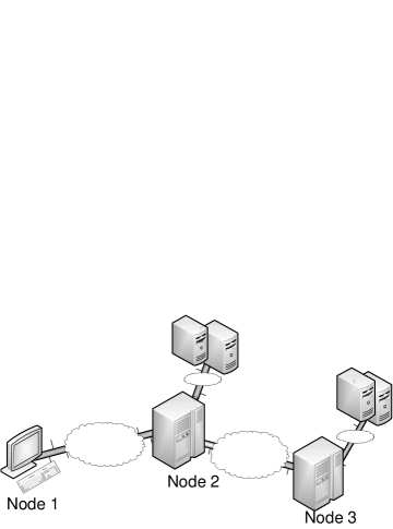
Figure 1: A multi-hop computer network in which intermediate and end nodes can access side information by interrogating remote data bases via cost-constrained actions.

As shown in [1] for a point-to-point system, the optimal operation of a VM at the decoder requires taking actions that are guided by the message received from the encoder. This implies the exchange of an explicit control signal embedded in the message communicated to the decoder that instructs the latter on how to operate the VM. Generalizing to the cascade models under study, a key issue to be tackled in this work is the design of communication strategies that strike the right balance between control signaling and source compression across the two hops.

I-A Related Work

As mentioned, the original paper [1] considered a point-to-point system with a single encoder and a single decoder. Various works have extended the results in [1] to multi-terminal models. Specifically, [5, 6] considered a set-up analogous to the Heegard-Berger problem [7, 8], in which the side information may or may not be available at the decoder. The more general case in which both decoders have access to the same vending machine, and either the side information produced by the vending machine at the two decoders satisfy a degradedness condition, or lossless source reconstructions are required at the decoders is solved in [5]. In [9], a distributed source coding setting that extends [10] to the case of a decoder with a side information VM is investigated, along with a cascade source coding model to be discussed below. Finally, in [11], a related problem is considered in which the sequence to be compressed is dependent on the actions taken by a separate encoder.

The problem of characterizing the rate-distortion region for cascade source coding models, even with conventional side information sequences (i.e., without VMs as in Fig. 2) at Node 2 and Node 3, is generally open. We refer to [2] and references therein for a review of the state of the art on the cascade problem and to [3] for the cascade-broadcast problem.

In this work, we focus on the cascade source coding problem with side information VMs. The basic cascade source coding model consists of three nodes arranged so that Node 1 communicates with Node 2 and Node 2 to Node 3 over finite-rate links, as illustrated for a computer network scenario in Fig. 1 and schematically in Fig. 2-(a). Both Node 2 and Node 3 wish to reconstruct a, generally lossy, version of source $X$ and have access to different side information sequences. An extension of the cascade model is the cascade-broadcast model of Fig. 2-(b), in which an additional "broadcast" link of rate $R_{b}$ exists that is received by both Node 2 and Node 3.

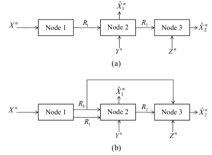
Figure 2: ($a$) Cascade source coding problem and ($b$) cascade-broadcast source coding problem.

Two specific instances of the models in Fig. 2 for which a characterization of the rate-distortion performance has been found are the settings considered in [4] and that in [12], which we briefly review here for their relevance to the present work. In [4], the cascade model in Fig. 2(a) was considered for the special case in which the side information $Y$ measured at Node 2 is also available at Node 1 (i.e., $X=(X,Y)$) and we have the Markov chain $X-Y-Z$ so that the side information at Node 3 is degraded with respect to that of Node 2. Instead, in [12], the cascade-broadcast model in Fig. 2(b) was considered for the special case in which either rate $R_{b}$ or $R_{1}$ is zero, and the reconstructions at Node 1 and Node 2 are constrained to be retrievable also at the encoder in the sense of the Common Reconstruction (CR) introduced in [13] (see below for a rigorous definition).

I-B Contributions

In this paper, we investigate the source coding models of Fig. 2 by assuming that some of the side information sequences can be affected by the actions taken by the corresponding nodes via VMs. The main contributions are as follows.

• Cascade source coding problem with VM at Node 3 (Fig. 3): In Sec. II-B, we derive the achievable rate-distortion-cost trade-offs for the set-up in Fig. 3, in which a side information VM exists at Node 3, while the side information $Y$ is known at both Node 1 and Node 2 and satisfies the Markov chain $X\textrm{---}Y\textrm{---}Z$. This characterization extends the result of [4] discussed above to a model with a VM at Node 3. We remark that in [9], the rate-distortion-cost characterization for the model in Fig. 3 was obtained, but under the assumption that the side information at Node 3 be available in a causal fashion in the sense of [14];

• Cascade-broadcast source coding problem with VM at Node 2 and Node 3, lossless compression (Fig. 4): In Sec. III-B, we study the cascade-broadcast model in Fig. 4 in which a VM exists at both Node 2 and Node 3. In order to enable the action to be taken by both Node 2 and Node 3, we assume that the information about which action should be taken by Node 2 and Node 3 is sent by Node 1 on the broadcast link of rate $R_{b}$. Under the constraint of lossless reconstruction at Node 2 and Node 3, we obtain a characterization of the rate-cost performance. This conclusion generalizes the result in [5] discussed above to the case in which the rate $R_{1}$ and/or $R_{2}$ are non-zero;

• Cascade-broadcast source coding problem with VM at Node 2 and Node 3, lossy compression with CR constraint (Fig. 4): In Sec. III-D, we tackle the problem in Fig. 4 but under the more general requirement of lossy reconstruction. Conclusive results are obtained under the additional constraints that the side information at Node 3 is degraded and that the source reconstructions at Node 2 and Node 3 can be recovered with arbitrarily small error probability at Node 1. This is referred to as the CR constraint following [13], and is of relevance in applications in which the data being sent is of sensitive nature and unknown distortions in the receivers’ reconstructions are not acceptable (see [13] for further discussion). This characterization extends the result of [12] mentioned above to the set-up with a side information VM, and also in that both rates $R_{1}$ and $R_{b}$ are allowed to be non-zero;

• Adaptive actions: Finally, we revisit the results above by allowing the decoders to select their actions in an adaptive way, based not only on the received messages but also on the previous samples of the side information extending [15]. Note that the effect of adaptive actions on rate–distortion–cost region was open even for simple point-to-point communication channel with decoder side non-causal side information VM until recently, when [15] has shown that adaptive action does not decrease the rate–distortion–cost region of point-to-point system. In this paper we have extended this result to the multi-terminal framework and we conclude that, in all of the considered examples, where applicable, adaptive

  

  Figure 3: Cascade source coding problem with a side information “vending machine” at Node 3.

  selection of the actions does not improve the achievable rate-distortion-cost trade-offs.

Our results extends to multi-hop scenarios the conclusion in [1] that a joint representation of data and control messages enables an efficient use of the available communication links. In particular, layered coding strategies prove to be optimal for all the considered models, in which, the base layer fulfills two objectives: determining the actions of downstream nodes and simultaneously providing a coarse description of the source. Moreover, the examples provided in the paper demonstrate the dependence of the optimal coding design on network topology action costs.

Throughout the paper, we closely follow the notation in [12]. In particular, a random variable is denoted by an upper case letter (e.g., $X,Y,Z$) and its realization is denoted by a lower case letter (e.g., $x,y,z$). The shorthand notation $X^{n}$ is used to denote the tuple (or the column vector) of random variables $(X_{1},\ldots,X_{n})$, and $x^{n}$ is used to denote a realization. The notation $X^{n}\sim p(x^{n})$ indicates that $p(x^{n})$ is the probability mass function (pmf) of the random vector $X^{n}$. Similarly, $Y^{n}|\{X^{n}=x^{n}\}\sim p(y^{n}|x^{n})$ indicates that $p(y^{n}|x^{n})$ is the conditional pmf of $Y^{n}$ given $\{X^{n}=x^{n}\}$. We say that $X\textrm{---}Y\textrm{---}Z$ form a Markov chain if $p(x,y,z)=p(x)p(y|x)p(z|y)$, that is, $X$ and $Z$ are conditionally independent of each other given $Y$.

II Cascade Source Coding with A Side information Vending Machine

In this section, we first describe the system model for the cascade source coding problem with a side information vending machine of Fig. 3. We then present the characterization of the corresponding rate-distortion-cost performance in Sec. II-B.

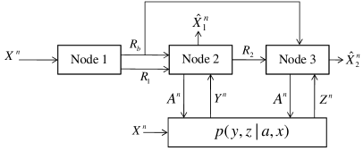
Figure 4: Cascade source coding problem with a side information “vending machine” at Node 2 and Node 3.

II-A System Model

The problem of cascade source coding of Fig. 3, is defined by the probability mass functions (pmfs) $p_{XY}(x,y)$ and $p_{Z|AY}(z|a,y)$ and discrete alphabets $\mathcal{X},\mathcal{Y},\mathcal{Z},\mathcal{A},\mathcal{\hat{X}}_{1},\mathcal{\hat{X}}_{2},$ as follows. The source sequences $X^{n}$ and $Y^{n}$ with $X^{n}\in\mathcal{X}^{n}$ and $Y^{n}\in\mathcal{Y}^{n}$, respectively, are such that the pairs $(X_{i},Y_{i})$ for $i\in[1,n]$ are independent and identically distributed (i.i.d.) with joint pmf $p_{XY}(x,y)$. Node 1 measures sequences $X^{n}$ and $Y^{n}$ and encodes them in a message $M_{1}$ of $nR_{1}$ bits, which is delivered to Node 2. Node 2 estimates a sequence $\hat{X}_{1}^{n}\in\mathcal{\hat{X}}_{1}^{n}$ within given distortion requirements to be discussed below. Moreover, Node 2 maps the message $M_{1}$ received from Node 1 and the locally available sequence $Y^{n}$ in a message $M_{2}$ of $nR_{2}$ bits, which is delivered to Node 3. Node 3 wishes to estimate a sequence $\hat{X}_{2}^{n}\in\mathcal{\hat{X}}_{2}^{n}$ within given distortion requirements. To this end, Node 3 receives message $M_{2}$ and based on this, it selects an action sequence $A^{n},$ where $A^{n}\in\mathcal{A}^{n}.$ The action sequence affects the quality of the measurement $Z^{n}$ of sequence $Y^{n}$ obtained at the Node 3. Specifically, given $A^{n}$ and $Y^{n}$, the sequence $Z^{n}$ is distributed as $p(z^{n}|a^{n},y^{n})=\prod_{i=1}^{n}p_{Z|A,Y}(z_{i}|y_{i},a_{i})$. The cost of the action sequence is defined by a cost function $\Lambda$: $\mathcal{A\rightarrow}[0,\Lambda_{\max}]$ with $0\leq\Lambda_{\max}<\infty,$ as $\Lambda(a^{n})=\sum_{i=1}^{n}\Lambda(a_{i})$. The estimated sequence $\hat{X}_{2}^{n}$ with $\hat{X}_{2}^{n}\in\mathcal{\hat{X}}_{2}^{n}$ is then obtained as a function of $M_{2}$ and $Z^{n}$. The estimated sequences $\hat{X}_{j}^{n}$ for $j=1,2$ must satisfy distortion constraints defined by functions $d_{j}(x,\hat{x}_{j})$: $\mathcal{X}\times\mathcal{\hat{X}}_{j}\rightarrow[0,D_{\max}]$ with $0\leq D_{\max}<\infty$ for $j=1,2,$ respectively. A formal description of the operations at the encoder and the decoder follows.

Figure 5: Cascade-broadcast source coding problem with a side information “vending machine” at Node 2.

Definition 1.

An $(n,R_{1},R_{2},D_{1},D_{2},\Gamma,\epsilon)$ code for the set-up of Fig. 3 consists of two source encoders, namely

$$\mathrm{g}_{1}\text{: }\mathcal{X}^{n}\times\mathcal{Y}^{n}\rightarrow[1,2^{nR_{1}}],$$ (1)

which maps the sequences $X^{n}$ and $Y^{n}$ into a message $M_{1};$

$$\mathrm{g}_{2}\text{:}\text{ }\mathcal{Y}^{n}\times[1,2^{nR_{1}}]\rightarrow[1,2^{nR_{2}}],$$ (2)

which maps the sequence $Y^{n}$ and message $M_{1}$ into a message $M_{2};$ an “action” function

$$\mathrm{\ell}\text{: }[1,2^{nR_{2}}]\rightarrow\mathcal{A}^{n},$$ (3)

which maps the message $M_{2}$ into an action sequence $A^{n};$ two decoders, namely

$$\mathrm{h}_{1}\text{: }[1,2^{nR_{1}}]\times\mathcal{Y}^{n}\rightarrow\mathcal{\hat{X}}_{1}^{n},$$ (4)

which maps the message $M_{1}$ and the measured sequence $Y^{n}$ into the estimated sequence $\hat{X}_{1}^{n};$

$$\mathrm{h}_{2}\text{: }[1,2^{nR_{2}}]\times\mathcal{Z}^{n}\rightarrow\mathcal{\hat{X}}_{2}^{n},$$ (5)

which maps the message $M_{2}$ and the measured sequence $Z^{n}$ into the the estimated sequence $\hat{X}_{2}^{n};$ such that the action cost constraint $\Gamma$ and distortion constraints $D_{j}$ for $j=1,2$ are satisfied, i.e.,

$$\frac{1}{n}\underset{i=1}{\overset{n}{\sum}}\mathrm{E}\left[\Lambda(A_{i})\right] \leq\Gamma$$ (6)

$$\text{ and }\frac{1}{n}\underset{i=1}{\overset{n}{\sum}}\mathrm{E}\left[d_{j}(X_{ji},\textrm{h}_{ji})\right] \leq D_{j}\text{ for }j=1,2,$$ (7)

where we have defined as $\textrm{h}_{1i}$ and $\textrm{h}_{2i}$ the $i$th symbol of the function $\textrm{h}_{1}(M_{1},Y^{n})$ and $\textrm{h}_{2}(M_{2},Z^{n})$, respectively.

Definition 2.

Given a distortion-cost tuple $(D_{1},D_{2},\Gamma)$, a rate tuple $(R_{1},R_{2})$ is said to be achievable if, for any $\epsilon>0$, and sufficiently large $n$, there exists a $(n,R_{1},R_{2},D_{1}+\epsilon,D_{2}+\epsilon,\Gamma+\epsilon)$ code.

Definition 3.

The rate-distortion-cost region $\mathcal{R}(D_{1},D_{2},\Gamma)$ is defined as the closure of all rate tuples $(R_{1},R_{2})$ that are achievable given the distortion-cost tuple $(D_{1},D_{2},\Gamma)$.

Remark 4.

For side information $Z$ available causally at Node 3, i.e., with decoding function (5) at Node 3 modified so that $\hat{X}_{i}$ is a function of $M_{2}$ and $Z^{i}$ only, the rate-distortion region $\mathcal{R}(D_{1},D_{2},\Gamma)$ has been derived in [9].

In the rest of this section, for simplicity of notation, we drop the subscripts from the definition of the pmfs, thus identifying a pmf by its argument.

II-B Rate-Distortion-Cost Region

In this section, a single-letter characterization of the rate-distortion-cost region is derived.

Proposition 5.

The rate-distortion-cost region $\mathcal{R\mbox{$(D_{1},D_{2},\Gamma)$}}$ for the cascade source coding problem illustrated in Fig. 3 is given by the union of all rate pairs $(R_{1},R_{2})$ that satisfy the conditions

$$R_{1} \geq I(X;\hat{X}_{1},A,U|Y)$$ (8a)

$$\ce{and}\mbox{ }R_{2} \geq I(X,Y;A)+I(X,Y;U|A,Z),$$ (8b)

where the mutual information terms are evaluated with respect to the joint pmf

$$p(x,y,z,a,\hat{x}_{1},u)=p(x,y)p(\hat{x}_{1},a,u|x,y)p(z|y,a)$$ , (9)

for some pmf $p(\hat{x}_{1},a,u|x,y)$ such that the inequalities

$$\ce{E}[d_{1}(X,\hat{X}_{1})] \leq D_{1},$$ (10a)

$$\ce{E}[d_{2}(X,\ce{f}(U,Z))] \leq D_{2},$$ (10b)

$$\ce{and}\textrm{ }\ce{E}[\Lambda(A)] \leq \Gamma,$$ (10c)

are satisfied for some function $\ce{f}\textrm{: }\mathcal{U}\times\mathcal{Z}\rightarrow\hat{\mathcal{X}}_{2}$. Finally, $U$ is an auxiliary random variable whose alphabet cardinality can be constrained as $|\mathcal{U}|\leq|\mathcal{X}||\mathcal{Y}||\mathcal{A}|+3$, without loss of optimality.

Remark 6.

For side information $Z$ independent of the action $A$ given $Y$, i.e., for $p(z|a,y)=p(z|y),$ the rate-distortion region $\mathcal{R}(D_{1},D_{2},\Gamma)$ in Proposition 5 reduces to that derived in [4].

The proof of the converse is provided in Appendix A for a more general case of adaptive action to be defined in Sec IV. The achievability follows as a combination of the techniques proposed in [1] and [4, Theorem 1]. Here we briefly outline the main ideas, since the technical details follow from standard arguments. For the scheme at hand, Node 1 first maps sequences $X^{n}$ and $Y^{n}$ into the action sequence $A^{n}$ using the standard joint typicality criterion. This mapping requires a codebook of rate $I(X,Y;A)$ (see, e.g., [16, pp. 62-63]). Given the sequence $A^{n}$, the sequences $X^{n}$ and $Y^{n}$ are further mapped into a sequence $U^{n}$. This requires a codebook of size $I(X,Y;U|A)$ for each action sequence $A^{n}$ from standard rate-distortion considerations [16, pp. 62-63]. Similarly, given the sequences $A^{n}$ and $U^{n},$ the sequences $X^{n}$ and $Y^{n}$ are further mapped into the estimate $\hat{X}_{1}^{n}$ for Node 2 using a codebook of rate $I(X,Y;\hat{X}_{1}|U,A)$ for each codeword pair $(U^{n},A^{n})$. The thus obtained codewords are then communicated to Node 2 and Node 3 as follows. By leveraging the side information $Y^{n}$ available at Node 2, conveying the codewords $A^{n},$ $U^{n}$ and $\hat{X}_{1}^{n}$ to Node 2 requires rate $I(X,Y;U,A)+I(X,Y;\hat{X}_{1}|U,A)-I(U,A,\hat{X}_{1};Y)$ by the Wyner-Ziv theorem [16, p. 280], which equals the right-hand side of (8a). Then, sequences $A^{n}$ and $U^{n}$ are sent by Node 2 to Node 3, which requires a rate equal to the right-hand side of (8b). This follows from the rates of the used codebooks and from the Wyner-Ziv theorem, due to the side information $Z^{n}$ available at Node 3 upon application of the action sequence $A^{n}$. Finally, Node 3 produces $\hat{X}_{2}^{n}$ that leverages through a symbol-by-symbol function as $\hat{X}_{2i}=\textrm{f}(U_{i},Z_{i})$ for $i\in[1,n].$

II-C Lossless Compression

Suppose that the source sequence $X^{n}$ needs to be communicated losslessly at both Node 2 and Node 3, in the sense that $d_{j}(x,\hat{x}_{j})$ is the Hamming distortion measure for $j=1,2$ ($d_{j}(x,\hat{x}_{j})=0$ if $x=\hat{x}_{j}$ and $d_{j}(x,\hat{x}_{j})=1$ if $x\neq\hat{x}_{j}$) and $D_{1}=D_{2}=0$. We can establish the following immediate consequence of Proposition 5.

Corollary 1.

The rate-distortion-cost region $\mathcal{R\mbox{$(0,0,\Gamma)$}}$ for the cascade source coding problem illustrated in Fig. 3 with Hamming distortion metrics is given by the union of all rate pairs $(R_{1},R_{2})$ that satisfy the conditions

$$R_{1} \geq I(X;A|Y)+H(X|A,Y)$$ (11a)

$$\ce{and}\mbox{ }R_{2} \geq I(X,Y;A)+H(X|A,Z),$$ (11b)

where the mutual information terms are evaluated with respect to the joint pmf

$$p(x,y,z,a)=p(x,y)p(a|x,y)p(z|y,a)$$ , (12)

for some pmf $p(a|x,y)$ such that $\ce{E}[\Lambda(A)]\leq\Gamma$.

III Cascade-Broadcast Source Coding with A Side Information Vending Machine

In this section, the cascade-broadcast source coding problem with a side information vending machine illustrated in Fig. 4 is studied. At first, the rate-cost performance is characterized for the special case in which the reproductions at Node 2 and Node 3 are constrained to be lossless. Then, the lossy version of the problem is considered in Sec. III-D, with an additional common reconstruction requirement in the sense of [13] and assuming degradedness of the side information sequences.

III-A System Model

In this section, we describe the general system model for the cascade-broadcast source coding problem with a side information vending machine. We emphasize that, unlike the setup of Fig. 3, here, the vending machine is at both Node 2 and Node 3. Moreover, we assume that an additional broadcast link of rate $R_{b}$ is available that is received by Node 2 and 3 to enable both Node 2 and Node 3 so as to take concerted actions in order to affect the side information sequences. We assume the action sequence taken by Node 2 and Node 3 to be a function of only the broadcast message $M_{b}$ sent over the broadcast link of rate $R_{b}$.

The problem is defined by the pmfs $p_{X}(x)$, $p_{YZ|AX}(y,z|a,x)$ and discrete alphabets $\mathcal{X},\mathcal{Y},{\cal Z},\mathcal{A},$ $\mathcal{\hat{X}}_{1},\mathcal{\hat{X}}_{2},$ as follows. The source sequence $X^{n}$ with $X^{n}\in\mathcal{X}^{n}$ is i.i.d. with pmf $p_{X}(x)$. Node 1 measures sequence $X^{n}$ and encodes it into messages $M_{1}$ and $M_{b}$ of $nR_{1}$ and $nR_{b}$ bits, respectively, which are delivered to Node 2. Moreover, message $M_{b}$ is broadcast also to Node 3. Node 2 estimates a sequence $\hat{X}_{1}^{n}\in\mathcal{\hat{X}}_{1}^{n}$ and Node 3 estimates a sequence $\hat{X}_{2}^{n}\in\mathcal{\hat{X}}_{2}^{n}$. To this end, Node 2 receives messages $M_{1}$ and $M_{b}$ and, based only on the latter message, it selects an action sequence $A^{n},$ where $A^{n}\in\mathcal{A}^{n}.$ Node 2 maps messages $M_{1}$ and $M_{b}$, received from Node 1, and the locally available sequence $Y^{n}$ in a message $M_{2}$ of $nR_{2}$ bits, which is delivered to Node 3. Node 3 receives messages $M_{2}$ and $M_{b}$ and based only on the latter message, it selects an action sequence $A^{n},$ where $A^{n}\in\mathcal{A}^{n}.$ Given $A^{n}$ and $X^{n}$, the sequences $Y^{n}$ and $Z^{n}$ are distributed as $p(y^{n},z^{n}|a^{n},x^{n})=\prod_{i=1}^{n}p_{YZ|A,X}(y_{i},z_{i}|a_{i},x_{i})$. The cost of the action sequence is defined as in previous section. A formal description of the operations at encoder and decoder follows.

Definition 7.

An $(n,R_{1},R_{2},R_{b},D_{1},D_{2},\Gamma,\epsilon)$ code for the set-up of Fig. 5 consists of two source encoders, namely

$$\mathrm{g}_{1}\text{: $\mathcal{X}^{n}\rightarrow[1,2^{nR_{1}}]\times[1,2^{nR_{b}}],$}$$ (13)

which maps the sequence $X^{n}$ into messages $M_{1}$ and $M_{b}$, respectively;

$$\mathrm{g}_{2}\text{:}\text{ }[1,2^{nR_{1}}]\times[1,2^{nR_{b}}]\times\mathcal{Y}^{n}\rightarrow[1,2^{nR_{2}}]$$ (14)

which maps the sequence $Y^{n}$ and messages $(M_{1},M_{b})$ into a message $M_{2};$ an “action” function

$$\mathrm{\ell}\text{: }[1,2^{nR_{b}}]\rightarrow\mathcal{A}^{n},$$ (15)

which maps the message $M_{b}$ into an action sequence $A^{n};$ two decoders, namely

$$\mathrm{h}_{1}\text{: }\text{ }[1,2^{nR_{1}}]\times[1,2^{nR_{b}}]\times\mathcal{Y}^{n}\rightarrow\mathcal{\hat{X}}_{1}^{n},$$ (16)

which maps messages $M_{1}$ and $M_{b}$ and the measured sequence $Y^{n}$ into the estimated sequence $\hat{X}_{1}^{n};$ and

$$\mathrm{h}_{2}\text{: }[1,2^{nR_{2}}]\times[1,2^{nR_{b}}]\times\mathcal{Z}^{n}\rightarrow\mathcal{\hat{X}}_{2}^{n},$$ (17)

which maps the messages $M_{2}$ and $M_{b}$ into the the estimated sequence $\hat{X}_{2}^{n};$ such that the action cost constraint (6) and distortion constraint (7) are satisfied.

Achievable rates $(R_{1},R_{2},R_{b})$ and rate-distortion-cost region are defined analogously to Definitions 2 and 3.

The rate–distortion–cost region for the system model described above is open even for the case without VM at Node 2 and Node 3 (see [3]). Hence, in the following subsections, we characterize the rate region for a few special cases. As in the previous section, subscripts are dropped from the pmf for simplicity of notation.

III-B Lossless Compression

In this section, a single-letter characterization of the rate-cost region $\mathcal{R\mbox{$(0,0,\Gamma)$}}$ is derived for the special case in which the distortion metrics are assumed to be Hamming and the distortion constraints are $D_{1}=0$ and $D_{2}=0$.

Proposition 8.

The rate-cost region $\mathcal{R\mbox{$(0,0,\Gamma)$}}$ for the cascade-broadcast source coding problem illustrated in Fig. 4 with Hamming distortion metrics is given by the union of all rate triples $(R_{1},R_{2},R_{b})$ that satisfy the conditions

$$R_{b} \geq I(X;A)$$ (18a)

$$R_{1}+R_{b} \geq I(X;A)+H(X|A,Y)$$ (18b)

$$\ce{and}\mbox{ }R_{2}+R_{b} \geq I(X;A)+H(X|A,Z)$$ (18c)

where the mutual information terms are evaluated with respect to the joint pmf

$$p(x,y,z,a)=p(x,a)p(y,z|a,x),$$ (19)

for some pmf $p(a|x)$ such that $\textrm{E}[\Lambda(A)]\leq\Gamma$.

Remark 9.

If $R_{1}=0$ and $R_{2}=0,$ the rate-cost region $\mathcal{R}(\Gamma)$ of Proposition 8 reduces to the one derived in [5, Theorem 1].

Remark 10.

The rate region (18) also describes the rate-distortion region under the more restrictive requirement of lossless reconstruction in the sense of the probabilities of error $\textrm{Pr}[X^{n}\neq\hat{X}_{j}^{n}]\leq\epsilon$ for $j=1,2$, as it follows from standard arguments (see [16, Sec. 3.6.4]). A similar conclusion applies for Corollary 1.

The converse proof for bound (18a) follows immediately since $A^{n}$ is selected only as a function of message $M_{b}$. As for the other two bounds, namely (18b)-(18c), the proof of the converse can be established following cut-set arguments and using the point-to-point result of [1]. For achievability, we use the code structure proposed in [1] along with rate splitting. Specifically, Node 1 first maps sequence $X^{n}$ into the action sequence $A^{n}$. This mapping requires a codebook of rate $I(X;A)$. This rate has to be conveyed over link $R_{b}$ by the definition of the problem and is thus received by both Node 2 and Node 3. Given the so obtained sequence $A^{n}$, communicating $X$ losslessly to Node 2 requires rate $H(X|A,Y)$. We split this rate into two rates $r_{1b}$ and $r_{1d}$, such that the message corresponding to the first rate is carried over the broadcast link of rate $R_{b}$ and the second on the direct link of rate $R_{1}$. Note that Node 2 can thus recover sequence $X$ losslessly. The rate $H(X|A,Z)$ which is required to send $X$ losslessly to Node 3, is then split into two parts, of rates $r_{2b}$ and $r_{2d}$. The message corresponding to the rate $r_{2b}$ is sent to Node 3 on the broadcast link of the rate $R_{b}$ by Node 1, while the message of rate $r_{2d}$ is sent by Node 2 to Node 3. This way, Node 1 and Node 2 cooperate to transmit $X$ to Node 3. As per the discussion above, the following inequalities have to be satisfied

$$r_{2b}+r_{2d}+r_{1b} \geq H(X|A,Z),$$

$$r_{1b}+r_{1d} \geq H(X|A,Y),$$

$$R_{1} \geq r_{1d},$$

$$R_{2} \geq r_{2d},$$

$$\textrm{and }R_{b} \geq r_{1b}+r_{2b}+I(X;A),$$

Applying Fourier-Motzkin elimination [16, Appendix C] to the inequalities above, the inequalities in (18) are obtained.

III-C Example: Switching-Dependent Side Information

We now consider the special case of the model in Fig. 4 in which the actions $A\in{\cal A}=\{0,1,2,3\}$ acts a switch that decides whether Node 2, Node 3 or either node gets to observe a side information $W$. The side information $W$ is jointly distributed with source $X$ according to the joint pmf $p(x,w)$. Moreover, defining as e an "erasure" symbol, the conditional pmf $p(y,z|x,a)$ is as follows: $Y=Z=\textrm{e}$ for $A=0$ (neither Node 2 nor Node 3 observes the side information $W$); $Y=W$ and $Z=\textrm{e}$ for $A=1$ (only Node 2 observes the side information $W$); $Y=\textrm{e}$ and $Z=W$ for $A=2$ (only Node 3 observes the side information $W$); and $Y=Z=W$ for $A=3$ (both nodes observe the side information $W$). We also select the cost function such that $\Lambda(j)=\lambda_{j}$ for $j\in{\cal A}$. When $R_{1}=R_{2}=0$, this model reduces to the ones studied in [5, Sec. III]. The following is a consequence of Proposition 2.

Corollary 11.

For the setting of switching-dependent side information described above, the rate-cost region (18) is given by

$$R_{b} \geq I(X;A)$$ (20a)

$$R_{1}+R_{b} \geq H(X)-p_{1}I(X;W|A=1)-p_{3}I(X;W|A=3)$$ (20b)

$$\ce{and}\mbox{ }R_{2}+R_{b} \geq H(X)-p_{2}I(X;W|A=2)-p_{3}I(X;W|A=3)$$ (20c)

where the mutual information terms are evaluated with respect to the joint pmf

$$p(x,y,z,a)=p(x,a)p(y,z|a,x),$$ (21)

for some pmf $p(a|x)$ such that $\sum_{j=0}^{3}p_{j}\lambda_{j}\leq\Gamma$, where we have denoted $p_{j}=\ce{Pr}[A=j]$ for $j\in{\cal A}$.

Proof:

The region (20) is obtained from the rate-cost region (18) by noting that in (18b) we have $I(X;A)+H(X|A,Y)=H(X)-I(X;Y|A)$ and similarly for (18c). ∎

In the following, we will elaborate upon two specific instances of the switching-dependent side information example.

Binary Symmetric Channel (BSC) between $X$ and $W$: Let $(X,W)$ be binary and symmetric so that $p(x)=p(w)=1/2$ for $x,w\in\{0,1\}$ and $\Pr[X\neq W]=\delta$ for $\delta\in[0,1]$. Moreover, let $\lambda_{j}=\infty$ for $j=0,3$ and $\lambda_{j}=1$ otherwise. We set the action cost constraint to $\Gamma=1$. Note that, given this definition of $\Lambda(a)$, at each time, Node 1 can choose whether to provide the side information $W$ to Node 2 or to Node 3 with no further constraints. By symmetry, it can be seen that we can set the pmf $p(a|x)$ with $x\in\{0,1\}$ and $a\in\{1,2\}$ to be a BSC with transition probability $q$. This implies that $p_{1}=\textrm{Pr}[A=1]=q$ and $p_{2}=\textrm{Pr}[A=2]=1-q$. We now evaluate the inequality (20a) as $R_{b}\geq 0$; inequality (20b) as $R_{1}+R_{b}\geq 1-p_{1}I(X;W|A=1)=1-qH(\delta)$; and similarly inequality (18c) as $R_{2}+R_{b}\geq 1-(1-q)H(\delta).$ From these inequalities, it can be seen that, in order to trace the boundary of the rate-cost region, in general, one needs to consider all values of $q$ in the interval $[0,1]$. This

Figure 6: The side information S-channel $p(w|x)$ used in the example of Sec. III-C.

corresponds to appropriate time-sharing between providing side information to Node 2 (for a fraction of time $q$) and Node 3 (for the remaining fraction of time). Note that, as shown in [5, Sec. III], if $R_{1}=R_{2}=0$, it is optimal to set $q=\frac{1}{2}$, and thus equally share the side information between Node 2 and Node 3, in order to minimize the rate $R_{b}$. This difference is due to the fact that in the cascade model at hand, it can be advantageous to provide more side information to one of the two encoders depending on the desired trade-off between the rates $R_{1}$ and $R_{2}$ in the achievable rate-cost region.

S-Channel between $X$ and $W$: We now consider the special case of Corollary 11 in which $(X,W)$ are jointly distributed so that $p(x)=1/2$ and $p(w|x)$ is the S-channel characterized by $p(0|0)=1-\delta$ and $p(1|1)=1$ (see Fig. 6). Moreover, we let $\lambda_{1}=1$, $\lambda_{2}=0$, $\lambda_{0}=\lambda_{3}=\infty$ as above, while the cost constraint is set to $\Gamma\leq 1$. As discussed in [5, Sec. III] for this example with $R_{1}=R_{2}=0$, providing side information to Node 2 is more costly and thus should be done efficiently. In particular, given Fig. 6, it is expected that biasing the choice $A=2$ when $X=1$ (i.e., providing side information to Node 2) may lead to some gain (see [5]). Here we show that in the cascade model, this gain depends on the relative importance of rates $R_{1}$ and $R_{2}$.

To this end, we set $p(a|x)$ as $p(1|0)=\alpha$ and $p(1|1)=\beta$ for $\alpha,\beta\in[0,1]$. We now evaluate the inequality (20a) as $R_{b}\geq 0$; inequality (20b) as

$$R_{1}+R_{b} \geq 1-\Bigl{(}\frac{\alpha+\beta}{2}\Bigr{)}\Bigl{(}H\Bigl{(}\frac{(1-\delta)\alpha}{\alpha+\beta}\Bigr{)}-H(1-\delta)\frac{\alpha}{\alpha+\beta}\Bigr{)};$$ (22)

and inequality (20c) as

$$R_{2}+R_{b} \geq 1-\Bigl{(}\frac{2-\alpha-\beta}{2}\Bigr{)}\Bigl{(}H\Bigl{(}\frac{(1-\delta)(1-\alpha)}{2-\alpha-\beta}\Bigr{)}-H(1-\delta)\frac{1-\alpha}{2-\alpha-\beta}\Bigr{)},$$ (23)

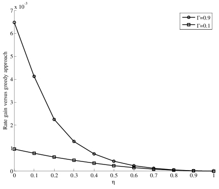
Figure 7: Difference between the weighted sum-rate $R_{1}+\eta R_{2}$ obtained with the greedy and with the optimal strategy as per Corollary 11 ($R_{b}=0.4$, $\delta=0.6$).

We now evaluate the minimum weighted sum-rate $R_{1}+\eta R_{2}$ obtained from (22)-(23) for $R_{b}=0.4$, $\delta=0.6$ and both $\Gamma=0.1$ and $\Gamma=0.9$. Parameter $\eta\geq 0$ rules on the relative importance of the two rates. For comparison, we also compute the performance attainable by imposing that the action $A$ be selected independent of $X$, which we refer to as the greedy approach [1]. Fig. 7 plots the difference between the two weighted sum-rates $R_{1}+\eta R_{2}$ . It can be seen that, as $\eta$ decreases and thus minimizing rate $R_{1}$ to Node 2 becomes more important, one can achieve larger gains by choosing the action $A$ to be dependent on $X$. Moreover, this gain is more significant when the action cost budget $\Gamma$ allows Node 2 to collect a larger fraction of the side information samples.

III-D Lossy Compression with Common Reconstruction Constraint

In this section, we turn to the problem of characterizing the rate-distortion-cost region ${\cal R}(D_{1},D_{2}$ $,\Gamma)$ for $D_{1},D_{2}>0$. In order to make the problem tractable , we impose the degradedness condition $X-(A,Y)-Z$ (as in [5]), which implies the factorization

$$p(y,z|a,x) = p(y|a,x)p(z|y,a);$$ (24)

and that the reconstructions at Nodes 2 and 3 be reproducible by Node 1. As discussed, this latter condition is referred to as the CR constraint [13]. Note that this constraint is automatically satisfied in the lossless case. To be more specific, an $(n,R_{1},R_{2},R_{b},D_{1},D_{2},\Gamma,\epsilon)$ code is defined per Definition 7 with the difference that there are two additional functions for the encoder, namely

$$\psi_{1}\textrm{: }\mathcal{X}^{n}\rightarrow\mathcal{\hat{X}}_{1}^{n}$$ (25a)

and $$\psi_{2}\textrm{: }\mathcal{X}^{n}\rightarrow\mathcal{\hat{X}}_{2}^{n},$$ (25b)

which map the source sequence into the estimated sequences at the encoder, namely $\psi_{1}(X^{n})$ and $\psi_{2}(X^{n})$, respectively; and the CR requirements are imposed, i.e.,

$$\textrm{Pr}\left[\psi_{1}(X^{n})\neq\textrm{h}_{1}(M_{1},M_{b},Y^{n})\right] \leq \epsilon$$ (26a)

$$\textrm{and Pr}\left[\psi_{2}(X^{n})\neq\textrm{h}_{2}(M_{2},M_{b},Z^{n})\right] \leq \epsilon,$$ (26b)

so that the encoder’s estimates $\psi_{1}(\cdot$) and $\psi_{2}(\cdot)$ are equal to the decoders’ estimates (cf. (16)-(17)) with high probability.

Proposition 12.

The rate-distortion region $\mathcal{R\mbox{$(D_{1},D_{2},\Gamma)$}}$ for the cascade-broadcast source coding problem illustrated in Fig. 4 under the CR constraint and the degradedness condition (24) is given by the union of all rate triples $(R_{1},R_{2},R_{b})$ that satisfy the conditions

$$R_{b} \geq I(X;A)$$ (27a)

$$R_{1}+R_{b} \geq I(X;A)+I(X;\hat{X}_{1},\hat{X}_{2}|A,Y)$$ (27b)

$$R_{2}+R_{b} \geq I(X;A)+I(X;\hat{X}_{2}|A,Z)$$ (27c)

$$\mbox{and}\mbox{ }R_{1}+R_{2}+R_{b} \geq I(X;A)+I(X;\hat{X}_{2}|A,Z)+I(X;\hat{X}_{1}|A,Y,\hat{X}_{2}),$$ (27d)

where the mutual information terms are evaluated with respect to the joint pmf

$$p(x,y,z,a,\hat{x}_{1},\hat{x}_{2})=p(x)p(a|x)p(y|x,a)p(z|a,y)p(\hat{x}_{1},\hat{x}_{2}|x,a)$$ , (28)

such that the inequalities

$$\ce{E}[d_{j}(X,\hat{X}_{j})] \leq D_{j}\textrm{, }\;\mbox{for }j=1,2,$$ (29a)

$$\mbox{and}\textrm{ }\ce{E}[\Lambda(A)] \leq \Gamma,$$ (29b)

are satisfied.

Remark 13.

If either $R_{1}=0$ or $R_{b}=0$ and the side information $Y$ is independent of the action $A$ given $X$, i.e., $\ p(y|a,x)=p(y|x),$ the rate-distortion region $\mathcal{R}(D_{1},D_{2},\Gamma)$ of Proposition 12 reduces to the one derived in [12, Proposition 10].

The proof of the converse is provided in Appendix B. The achievability follows similar to Proposition 8. Specifically, Node 1 first maps sequence $X^{n}$ into the action sequence $A^{n}$. This mapping requires a codebook of rate $I(X;A)$. This rate has to be conveyed over link $R_{b}$ by the definition of the problem and is thus received by both Node 2 and Node 3. The source sequence $X^{n}$ is mapped into the estimate $\hat{X}_{2}^{n}$ for Node 3 using a codebook of rate $I(X;\hat{X}_{2}|A)$ for each sequence $A^{n}$. Communicating $\hat{X}_{2}^{n}$ to Node 2 requires rate $I(X;\hat{X}_{2}|A,Y)$ by the Wyner-Ziv theorem. We split this rate into two rates $r_{2b}$ and $r_{2d}$, such that the message corresponding to the first rate is carried over the broadcast link of rate $R_{b}$ and the second on the direct link of rate $R_{1}$. Note that Node 2 can thus recover sequence $\hat{X}_{2}^{n}$. Communicating $\hat{X}_{2}^{n}$ to Node 3 requires rate $I(X;\hat{X}_{2}|A,Z)$ by the Wyner-Ziv theorem. We split this rate into two rates $r_{0b}$ and $r_{0d}$. The message corresponding to the rate $r_{0b}$ is send to Node 3 on the broadcast link of the rate $R_{b}$ by Node 1, while the message of rate $r_{0d}$ is sent by Node 2 to Node 3. This way, Node 1 and Node 2 cooperate to transmit $\hat{X}_{2}$ to Node 3. Finally, the source sequence $X^{n}$ is mapped by Node 1 into the estimate $\hat{X}_{1}^{n}$ for Node 2 using a codebook of rate $I(X;\hat{X}_{1}|A,\hat{X}_{2})$ for each pair of sequences $(A^{n},\hat{X}_{2}^{n})$. Using the Wyner-Ziv coding, this rate is reduced to $I(X;\hat{X}_{1}|A,Y,\hat{X}_{2})$ and split into two rates $r_{1b}$ and $r_{1d}$, which are sent through links $R_{b}$ and $R_{1}$, respectively. As per discussion above, the following inequalities have to be satisfied

$$r_{0b}+r_{0d}+r_{2b} \geq I(X;\hat{X}_{2}|A,Z),$$

$$r_{2b}+r_{2d} \geq I(X;\hat{X}_{2}|A,Y),$$

$$r_{1b}+r_{1d} \geq I(X;\hat{X}_{1}|A,Y,\hat{X}_{2}),$$

$$R_{1} \geq r_{1d}+r_{2d},$$

$$R_{2} \geq r_{0d},$$

$$\textrm{and }R_{b} \geq r_{1b}+r_{2b}+r_{0b}+I(X;A),$$

Applying Fourier-Motzkin elimination [16, Appendix C] to the inequalities above, the inequalities in (27) are obtained.

IV Adaptive Actions

In this section, we assume that actions taken by the nodes are not only a function of the message $M_{2}$ for the model of Fig. 3 or $M_{b}$ for the models of Fig. 4 and Fig. 5, respectively, but also a function of the past observed side information samples. Following [15], we refer to this case as the one with adaptive actions. Note that for the cascade-broadcast problem, we consider the model in Fig. 5, which differs from the one in Fig. 4 considered thus far in that the side information $Z$ is not available at Node 3. At this time, it appears to be problematic to define adaptive actions in the presence of two nodes that observe different side information sequences. For the cascade model in Fig. 3, a $(n,R_{1},R_{2},D_{1},D_{2},\Gamma)$ code is defined per Definition 1 with the difference that the action encoder (3) is modified to be

$$\mathrm{\ell}\text{: }[1,2^{nR_{2}}]\times{\cal Z}^{i-1}\rightarrow\mathcal{A},$$ (30)

which maps the message $M_{2}$ and the past observed decoder side information sequence $Z^{i-1}$ into the $i$th symbol of the action sequence $A_{i}$. Moreover, for the cascade-broadcast model of Fig. 5, the “action” function (15) in Definition 7 is modified as

$$\mathrm{\ell}\text{: }[1,2^{nR_{b}}]\times{\cal Y}^{i-1}\rightarrow\mathcal{A},$$ (31)

which maps the message $M_{b}$ and the past observed decoder side information sequence $Y^{i-1}$ into the $i$th symbol of the action sequence $A_{i}$.

Proposition 14.

The rate-distortion-cost region $\mathcal{R\mbox{$(D_{1},D_{2},\Gamma)$}}$ for the cascade source coding problem illustrated in Fig. 3 with adaptive action-dependent side information is given by the rate region described in Proposition 5.

Proposition 15.

The rate-distortion-cost region $\mathcal{R\mbox{$(D_{1},D_{2},\Gamma)$}}$ for the cascade-broadcast source coding problem under the CR illustrated in Fig. 5 with adaptive action-dependent side information is given by the region described in Proposition 12 by setting $Z=\emptyset$.

Remark 16.

The results above show that enabling adaptive actions does not increase the achievable rate-distortion-cost region. These results generalize the observations in [15] for the point-to-point setting, wherein a similar conclusion is drawn.

To establish the propositions above, we only need to prove the converse. The proofs for Proposition 14 and Proposition 15 are given in Appendix A and B, respectively.

V Concluding Remarks

In an increasing number of applications, communication networks are expected to be able to convey not only data, but also information about control for actuation over multiple hops. In this work, we have tackled the analysis of a baseline communication model with three nodes connected in a cascade with the possible presence of an additional broadcast link. We have characterized the optimal trade-off between rate, distortion and cost for actuation in a number of relevant cases of interest. In general, the results point to the advantages of leveraging a joint representation of data and control information in order to utilize in the most efficient way the available communication links. Specifically, in all the considered models, a layered coding strategy, possibly coupled with rate splitting, has been proved to be optimal. This strategy is such that the base layer has the double role of guiding the actions of the downstream nodes and of providing a coarse description of the source, similar to [1]. Moreover, it is shown that this base compression layer should be designed in a way that depends on the network topology and on the relative cost of activating the different links.

VI ACKNOWLEDGMENTS

The work of O. Simeone is supported by the U.S. National Science Foundation under grant CCF-0914899, and the work of U. Mitra by ONR N00014-09-1-0700, NSF CCF-0917343 and DOT CA-26-7084-00.

Appendix A: Converse Proof for Proposition 5 and 14

Here, we prove the converse part of Proposition 14. Since the setting of Proposition 5 is more restrictive, as it does not allow for adaptive actions, the converse proof for Proposition 5 follows immediately. For any $(n,R_{1},R_{2},D_{1}+\epsilon,D_{2}+\epsilon,\Gamma+\epsilon)$ code, we have

$$nR_{1} \geq H(M_{1})$$

$$\geq H(M_{1}|Y^{n})$$

$$\stackrel{{\scriptstyle(a)}}{{=}}I(M_{1};X^{n},Z^{n}|Y^{n})$$

$$=H(X^{n},Z^{n}|Y^{n})-H(X^{n},Z^{n}|M_{1},Y^{n})$$

$$=H(X^{n}|Y^{n})+H(Z^{n}|X^{n},Y^{n})-H(Z^{n}|Y^{n},M_{1})-H(X^{n}|Z^{n},Y^{n},M_{1})$$

$$\stackrel{{\scriptstyle(a,b)}}{{=}}H(X^{n}|Y^{n})+H(Z^{n}|X^{n},Y^{n},M_{1},M_{2})-H(Z^{n}|Y^{n},M_{1},M_{2})-H(X^{n}|Z^{n},Y^{n},M_{1},M_{2})$$

$$\stackrel{{\scriptstyle(c)}}{{=}}H(X^{n}|Y^{n})-H(X^{n}|Z^{n},Y^{n},M_{1},M_{2},A^{n},\hat{X}_{1}^{n})$$

$$+\sum_{i=1}^{n}H(Z_{i}|Z^{i-1},X^{n},Y^{n},M_{1},M_{2})-H(Z_{i}|Z^{i-1},Y^{n},M_{1},M_{2})$$

$$\stackrel{{\scriptstyle(c,d)}}{{\geq}}\sum_{i=1}^{n}(H(X_{i}|Y_{i})-H(X_{i}|X^{i-1},Y^{i},M_{2},A^{i},Z^{n},\hat{X}_{1i}))$$

$$+\sum_{i=1}^{n}H(Z_{i}|Z^{i-1},X^{n},Y^{n},M_{1},M_{2},A_{i})-H(Z_{i}|Z^{i-1},Y^{n},M_{1},M_{2},A_{i})$$

$$\stackrel{{\scriptstyle(e)}}{{=}}\sum_{i=1}^{n}I(X_{i};\hat{X}_{1i},A_{i},U_{i}|Y_{i})+H(Z_{i}|Y_{i},A_{i})-H(Z_{i}|Y_{i},A_{i})$$

$$=\sum_{i=1}^{n}I(X_{i};\hat{X}_{1i},A_{i},U_{i}|Y_{i}),$$ (32)

where $(a)$ follows since $M_{1}$ is a function of $(X^{n},Y^{n})$; $(b)$ follows since $M_{2}$ is a function of $(M_{1},Y^{n})$; $(c)$ follows since $A_{i}$ is a function of $(M_{2},Z^{i-1})$ and since $\hat{X}_{1}^{n}$ is a function of $(M_{1},Y^{n})$; $(d)$ follows since conditioning decreases entropy and since $X^{n}$ and $Y^{n}$ are i.i.d.; and $(e)$ follows by defining $U_{i}=(M_{2},X^{i-1},Y^{i-1},A^{i-1},Z^{n\backslash i})$ and since $(Z^{i-1},X^{n},Y^{n\backslash i},M_{1},M_{2})\textrm{---}$ $(A_{i},Y_{i})\textrm{---}Z_{i}$ form a Markov chain by construction. We also have

$$nR_{2} \geq H(M_{2})$$

$$= I(M_{2};X^{n},Y^{n},Z^{n})$$

$$= H(X^{n},Y^{n},Z^{n})-H(X^{n},Y^{n},Z^{n}|M_{2})$$ (33)

$$= H(X^{n},Y^{n})+H(Z^{n}|X^{n},Y^{n})-H(Z^{n}|M_{2})-H(X^{n},Y^{n}|M_{2},Z^{n})$$

$$= \overset{n}{\underset{i=1}{\sum}}H(X_{i},Y_{i})+H(Z_{i}|Z^{i-1},X^{n},Y^{n})-H(Z_{i}|Z^{i-1},M_{2})$$

$$-H(X_{i},Y_{i}|X^{i-1},Y^{i-1},M_{2},Z^{n})$$

$$\overset{(a)}{=} \overset{n}{\underset{i=1}{\sum}}H(X_{i},Y_{i})\negmedspace+\negmedspace H(Z_{i}|Z^{i-1},X^{n},Y^{n},M_{2},A_{i})\negmedspace-\negmedspace H(Z_{i}|Z^{i-1},M_{2},A_{i})\negmedspace$$

$$-\negmedspace H(X_{i},Y_{i}|X^{i-1},Y^{i-1},M_{2},Z^{n},A^{i})$$

$$\overset{(b)}{\geq} \overset{n}{\underset{i=1}{\sum}}H(X_{i},Y_{i})+H(Z_{i}|X_{i},Y_{i},A_{i})-H(Z_{i}|A_{i})-H(X_{i},Y_{i}|U_{i},A_{i},Z_{i}),$$

where (a) follows because $M_{2}$ is a function of $(M_{1},Y^{n})$ and thus of $(X^{n},Y^{n})$ and because $A^{i}$ is a function of $(M_{2},Z^{i-1})$ and ($b$) follows since conditioning decreases entropy, since the Markov chain relationship $Z_{i}\textrm{---}(X_{i},Y_{i},A_{i})\textrm{---}$ $(X^{n\backslash i},Y^{n\backslash i},M_{2})$ holds and by using the definition of $U_{i}$.

Defining $Q$ to be a random variable uniformly distributed over $[1,n]$ and independent of all the other random variables and with $X\overset{\triangle}{=}X_{Q}$, $Y\overset{\triangle}{=}Y_{Q}$, $Z\overset{\triangle}{=}Z_{Q}$, $A\overset{\triangle}{=}A_{Q}$, $\hat{X}_{1}\overset{\triangle}{=}\hat{X}_{1Q}$, $\hat{X}_{2}\overset{\triangle}{=}\hat{X}_{2Q}$ and $U\overset{\triangle}{=}(U_{Q},Q),$ from (32) we have

$$nR_{1} \geq I(X;\hat{X}_{1},A,U|Y,Q)\overset{(a)}{\geq}H(X|Y)-H(X|\hat{X}_{1},A,U,Y)=I(X;\hat{X}_{1},A,U|Y),$$

where in ($a$) we have used the fact that $(X^{n},Y^{n})$ are i.i.d and conditioning reduces entropy. Moreover, from (33) we have

$$nR_{2} \geq H(X,Y|Q)+H(Z|X,Y,A,Q)-H(Z|A,Q)-H(X,Y|U,A,Z,Q)$$

$$\overset{(a)}{\geq} H(XY)+H(Z|X,Y,A)-H(Z|A)-H(X,Y|U,A,Z)$$

$$= I(XY;U,A,Z)-I(Z;X,Y|A)$$

$$= I(XY;A)+I(X,Y;U|A,Z),$$

where ($a$) follows since $(X^{n},Y^{n})$ are i.i.d, since conditioning decreases entropy, by the definition of $U$ and by the problem definition. We note that the defined random variables factorize as (9) since we have the Markov chain relationship $X$—$(A,Y)$—$Z$ by the problem definition and that $\hat{X}_{2}$ is a function $\textrm{f}(U,Z)$ of $U$ and $Z$ by the definition of $U$. Moreover, from the cost and distortion constraints (6)-(7), we have

$$D_{j}+\epsilon \geq\textrm{$\frac{1}{n}\sum_{i=1}^{n}$E}[d_{j}(X_{i},\hat{X}_{ji})]=\textrm{E}[d_{j}(X,\hat{X}_{j})],\textrm{ for }j=1,2,$$ (34a)

$$\textrm{and }\Gamma+\epsilon \geq\frac{1}{n}\sum_{i=1}^{n}\textrm{E}\left[\Lambda(A_{i})\right]=\textrm{E}\left[\Lambda(A)\right].$$ (34b)

To bound the cardinality of auxiliary random variable $U$, we fix $p(z|y,a)$ and factorize the joint pmf $p(x,y,z,a,u,\hat{x}_{1})$ as

$$p(x,y,z,a,u,\hat{x}_{1}) = p(u)p(\hat{x}_{1},a,x,y|u)p(z|y,a).$$

Therefore, for fixed $p(z|y,a)$, the quantities (8a)-(10c) can be expressed in terms of integrals given by $\int g_{j}(p(\hat{x}_{1},a,x,y|u))dF(u)$, for $j=1,...,|\mathcal{X}||\mathcal{Y}||\mathcal{A}|+3$, of functions $g_{j}(\cdot)$ that are continuous on the space of probabilities over alphabet $|\mathcal{X}|\text{\texttimes}|\mathcal{Y}|\text{\texttimes}|\mathcal{A}|\text{\texttimes}|\hat{\mathcal{X}}_{1}|$. Specifically, we have $g_{j}$ for $j=1,...,|\mathcal{X}||\mathcal{Y}||\mathcal{A}|-1$, given by the pmf $p(a,x,y)$ for all values of $x\in\mathcal{X}$, $y\in\mathcal{Y}$ and $a\in\mathcal{A}$, (except one), $g_{|\mathcal{X}||\mathcal{Y}||\mathcal{A}|}=H(X|A,Y,\hat{X}_{1},U=u)$, $g_{|\mathcal{X}||\mathcal{Y}||\mathcal{A}|+1}=H(X,Y|A,Z,U=u)$, and $g_{|\mathcal{X}||\mathcal{Y}||\mathcal{A}|+1+j}=\textrm{E}[d_{j}(X,\hat{X}_{j})|U=u],$ for $j=1,2$. The proof in concluded by invoking the Fenchel–Eggleston–Caratheodory theorem [16, Appendix C].

Appendix B: Proof of Proposition 12

Here, we prove the converse parts of Proposition 12 and Proposition 15. We start by proving Proposition 12. The proof of Proposition 15 will follow by setting $Z=\emptyset$, and noting that in the proof below the action $A_{i}$ can be made to be a function of $Y^{i-1}$, in addition to being a function of $M_{b}$, without modifying any steps of the proof. By the CR requirements (26), we first observe that for any $(n,R_{1},R_{2},R_{b},D_{1}+\epsilon,D_{2}+\epsilon,\Gamma+\epsilon)$ code, we have the Fano inequalities

$$H(\psi_{1}(X^{n})|\textrm{h}_{1}(M_{1},M_{b},Y^{n})) \leq n\delta(\epsilon),$$ (35a)

$$\textrm{and }H(\psi_{2}(X^{n})|\textrm{h}_{2}(M_{2},M_{b},Z^{n})) \leq n\delta(\epsilon),$$ (35b)

where $\delta(\epsilon)$ denotes any function such that $\delta(\epsilon)\rightarrow 0$ if $\epsilon\rightarrow 0$. Next, we have

$$nR_{b} \geq H(M_{b})$$

$$\stackrel{{\scriptstyle(a)}}{{=}}I(M_{b};X^{n},Y^{n})$$

$$=H(X^{n},Y^{n})-H(X^{n},Y^{n}|M_{b})$$

$$\stackrel{{\scriptstyle(a)}}{{=}}H(X^{n})+H(Y^{n}|X^{n},M_{b})-H(X^{n},Y^{n}|M_{b})$$

$$\stackrel{{\scriptstyle(b)}}{{=}}\sum_{i=1}^{n}H(X_{i})+H(Y_{i}|Y^{i-1},X^{n},M_{b},A_{i})-H(X_{i},Y_{i}|X^{i-1},Y^{i-1},M_{b},A_{i})$$

$$=\sum_{i=1}^{n}H(X_{i})+H(Y_{i}|Y^{i-1},X^{n},M_{b},A_{i})-H(X_{i}|X^{i-1},Y^{i-1},M_{b},A_{i})$$

$$-H(Y_{i}|X^{i},Y^{i-1},M_{b},A_{i})$$

$$\stackrel{{\scriptstyle(c)}}{{=}}\sum_{i=1}^{n}H(X_{i})+H(Y_{i}|X_{i},A_{i})-H(X_{i}|X^{i-1},Y^{i-1},M_{b},A_{i})-H(Y_{i}|X_{i},A_{i})$$

$$\stackrel{{\scriptstyle(d)}}{{\geq}}\sum_{i=1}^{n}H(X_{i})-H(X_{i}|A_{i}),$$ (36)

where $(a)$ follows since $M_{b}$ is a function of $X^{n}$; $(b)$ follows since $A_{i}$ is a function of $M_{b}$ and since $X^{n}$ is i.i.d.; $(c)$ follows since $(Y^{i-1},X^{n\backslash i},M_{b})\textrm{---}(A_{i},X_{i})\textrm{---}Y_{i}$ forms a Markov chain by problem definition; and $(d)$ follows conditioning reduces entropy. In the following, for simplicity of notation, we write $\textrm{h}_{1},\textrm{h}_{2},\psi_{1},\psi_{2}$ for the values of corresponding functions in Sec. III-D. Next, We can also write

$$n(R_{1}+R_{b}) \geq H(M_{1},M_{b})$$

$$\overset{(a)}{=} I(M_{1},M_{b};X^{n},Y^{n},Z^{n})$$

$$= H(X^{n},Y^{n},Z^{n})-H(X^{n},Y^{n},Z^{n}|M_{1},M_{b})$$

$$= H(X^{n})+H(Y^{n},Z^{n}|X^{n})-H(Y^{n},Z^{n}|M_{1},M_{b})-H(X^{n}|Y^{n},Z^{n},M_{1},M_{b})$$

$$\overset{(b)}{=} H(X^{n})+H(Y^{n},Z^{n}|X^{n},M_{b})-H(Y^{n}|M_{1},M_{b})$$

$$-H(Z^{n}|M_{1},M_{b},Y^{n},A^{n})-H(X^{n}|Y^{n},Z^{n},M_{1},M_{b},M_{2},A^{n})$$

$$\overset{(b,c)}{=} \overset{n}{\underset{i=1}{\sum}}H(X_{i})+H(Y_{i},Z_{i}|X_{i},A_{i})-H(Y_{i}|Y^{i-1},M_{1},M_{b},A_{i})$$

$$-H(Z_{i}|Z^{i-1},M_{1},M_{b},Y^{n},A^{n})-H(X_{i}|X^{i-1},Y^{n},Z^{n},M_{1},M_{b},A^{n},M_{2},\textrm{h}_{1},\textrm{h}_{2})$$

$$\overset{(d)}{\geq} \overset{n}{\underset{i=1}{\sum}}H(X_{i})\negmedspace+\negmedspace H(Y_{i}|X_{i},A_{i})+\negmedspace H(Z_{i}|Y_{i},A_{i})-H(Y_{i}|A_{i})-H(Z_{i}|Y_{i},A_{i})$$

$$-H(X_{i}|Y_{i},A_{i},\textrm{h}_{1},\textrm{h}_{2})\negmedspace$$

$$= \overset{n}{\underset{i=1}{\sum}}I(X_{i};Y_{i},A_{i},\textrm{h}_{1},\textrm{h}_{2})-I(Y_{i};X_{i}|A_{i})$$ (37)

$$= \overset{n}{\underset{i=1}{\sum}}I(X_{i};Y_{i},A_{i},\textrm{h}_{1},\textrm{h}_{2},\psi_{1},\psi_{2})-I(X_{i};\psi_{1},\psi_{2}|Y_{i},A_{i},\textrm{h}_{1},\textrm{h}_{2})-I(Y_{i};X_{i}|A_{i})$$

$$\overset{(e)}{\geq} \overset{n}{\underset{i=1}{\sum}}I(X_{i};Y_{i},A_{i},\psi_{1},\psi_{2})-H(\psi_{1},\psi_{2}|Y_{i},A_{i},\textrm{h}_{1},\textrm{h}_{2})$$

$$+H(\psi_{1},\psi_{2}|Y_{i},A_{i},\textrm{h}_{1},\textrm{h}_{2},X_{i})-I(Y_{i};X_{i}|A_{i})$$

$$\overset{(f)}{\geq} \overset{n}{\underset{i=1}{\sum}}I(X_{i};Y_{i},A_{i},\psi_{1},\psi_{2})-I(Y_{i};X_{i}|A_{i})+n\delta(\epsilon)$$

$$= \overset{n}{\underset{i=1}{\sum}}I(X_{i};A_{i})+I(X_{i};\psi_{1},\psi_{2}|Y_{i},A_{i})+n\delta(\epsilon),$$

where ($a$) follows because $(M_{1},M_{b})$ is a function of $X^{n}$; ($b$) follows because $M_{b}$ is a function of $X^{n}$, $A^{n}$ is a function of $M_{b}$ and $M_{2}$ is a function of $(M_{1},M_{b},Y^{n})$; ($c$) follows since $H(Y^{n},Z^{n}|X^{n},M_{b})=\sum_{i=1}^{n}H(Y_{i},Z_{i}|$ $Y^{i-1},Z^{i-1},X^{n},M_{b},A_{i})=\sum_{i=1}^{n}H(Y_{i},Z_{i}|X_{i},A_{i})$ and since $\textrm{h}_{1}$ and $\textrm{h}_{2}$ are functions of $(M_{1},M_{b},Y^{n})$ and $(M_{2},M_{b},Z^{n})$, respectively and because $(Y_{i},Z_{i})\textrm{---}(X_{i},A_{i})\textrm{---}$ $(X^{n\backslash i},Y^{i-1},Z^{i-1},M_{b})$ forms a Markov chain; ($d$) follows since conditioning reduces entropy, since side information VM follows $p(y^{n},z^{n}|a^{n},x^{n})$$=\prod_{i=1}^{n}p_{Y|A,X}(y_{i}|a_{i},x_{i})$ $p_{Z|A,Y}(z_{i}|a_{i},y_{i})$ from (24) and because $Z_{i}\textrm{---}(Y_{i},A_{i})\textrm{---}$ $(Y^{n\backslash i},Z^{i-1},M_{1},M_{b})$ forms a Markov chain; ($e$) follows by the chain rule for mutual information and the fact that mutual information is non-negative; and ($f$) follows by the Fano inequality (35) and because entropy is non-negative. We can also write

$$n(R_{2}+R_{b}) \geq H(M_{2},M_{b})$$

$$\stackrel{{\scriptstyle(a)}}{{=}} I(M_{2},M_{b};X^{n},Y^{n},Z^{n})$$

$$= H(X^{n},Y^{n},Z^{n})-H(X^{n},Y^{n},Z^{n}|M_{2},M_{b})$$

$$\stackrel{{\scriptstyle(a)}}{{=}} H(X^{n})+H(Y^{n},Z^{n}|X^{n},M_{b})-H(Z^{n}|M_{2},M_{b})-H(X^{n},Y^{n}|Z^{n},M_{2},M_{b})$$

$$\stackrel{{\scriptstyle(b)}}{{=}} \sum_{i=1}^{n}H(X_{i})+H(Y_{i},Z_{i}|Y^{i-1},Z^{i-1},X^{n},M_{b},A_{i})-H(Z_{i}|Z^{i-1},M_{2},M_{b},A_{i})$$

$$- H(X_{i},Y_{i}|X^{i-1},Y^{i-1},M_{2},M_{b},Z^{n},A_{i})$$

$$= \sum_{i=1}^{n}H(X_{i},Y_{i})-H(Y_{i}|X_{i})+H(Y_{i},Z_{i}|Y^{i-1},Z^{i-1},X^{n},M_{b},A_{i})$$

$$- H(Z_{i}|Z^{i-1},M_{2},M_{b},A_{i})-H(X_{i},Y_{i}|X^{i-1},Y^{i-1},M_{2},M_{b},Z^{n},A_{i})$$

$$\stackrel{{\scriptstyle(c)}}{{=}}\sum_{i=1}^{n}H(X_{i},Y_{i})-H(Y_{i}|X_{i})+H(Y_{i}|X_{i},A_{i})+H(Z_{i}|A_{i},Y_{i},X_{i})$$

$$-H(Z_{i}|Z^{i-1},M_{2},M_{b},A_{i})-H(X_{i},Y_{i}|X^{i-1},Y^{i-1},M_{2},M_{b},Z^{n},A_{i})$$

$$\stackrel{{\scriptstyle(d)}}{{=}}\sum_{i=1}^{n}H(X_{i},Y_{i})-I(Y_{i};A_{i}|X_{i})+H(Z_{i}|A_{i},Y_{i},X_{i})-H(Z_{i}|Z^{i-1},M_{2},M_{b},A_{i})$$

$$-H(X_{i},Y_{i}|X^{i-1},Y^{i-1},M_{2},M_{b},\textrm{h}_{2},Z^{n},A_{i})$$

$$\stackrel{{\scriptstyle(e)}}{{\geq}}\sum_{i=1}^{n}H(X_{i},Y_{i})+I(X_{i};A_{i})-I(Y_{i},X_{i};A_{i})+H(Z_{i}|A_{i},Y_{i},X_{i})$$

$$-H(Z_{i}|A_{i})-H(X_{i},Y_{i}|\textrm{h}_{2},A_{i},Z_{i})$$

$$=\sum_{i=1}^{n}I(X_{i},Y_{i};\textrm{h}_{2},A_{i},Z_{i},\psi_{2i})-I(X_{i},Y_{i};\psi_{2i}|\textrm{h}_{2},A_{i},Z_{i})+I(X_{i};A_{i})$$

$$-I(Y_{i},X_{i};A_{i})-I(X_{i},Y_{i};Z_{i}|A_{i})$$

$$\geq\sum_{i=1}^{n}I(X_{i},Y_{i};A_{i},Z_{i},\psi_{2i})-H(\psi_{2i}|\textrm{h}_{2},A_{i},Z_{i})+H(\psi_{2i}|\textrm{h}_{2},A_{i},X_{i},Y_{i},Z_{i})$$

$$+I(X_{i};A_{i})-I(X_{i},Y_{i};Z_{i},A_{i})$$

$$\stackrel{{\scriptstyle(f)}}{{\geq}}\sum_{i=1}^{n}I(X_{i};A_{i})+I(X_{i},Y_{i};\psi_{2i}|A_{i},Z_{i})+n\delta(\epsilon),$$ (38)

where $(a)$ follows since $M_{b}$ is a function of $X^{n}$ and because $M_{2}$ is a function of $(M_{1},M_{b},Y^{n})$ and thus of $(X^{n},Y^{n})$; $(b)$ follows since $A_{i}$ is a function of $M_{b}$ and since $X^{n}$ is i.i.d.; $(c)$ follows since $(Y_{i},Z_{i})\textrm{---}(X_{i},A_{i})\textrm{---}$ $(X^{n\backslash i},Y^{i-1},Z^{i-1},M_{b})$ forms a Markov chain and since $p(y^{n},z^{n}|a^{n},x^{n})$ $=\prod_{i=1}^{n}p_{Y|A,X}(y_{i}|a_{i},x_{i})$$p_{Z|A,Y}(z_{i}|a_{i},y_{i})$; $(d)$ follows since $\textrm{h}_{2}$ is a function of $(M_{2},M_{b},Z^{n})$; $(e)$ follows since conditioning reduces entropy; and $(f)$ follows since entropy is non-negative and using the Fanos inequality. Moreover, with the definition $M=(M_{1},M_{2},M_{b})$, we have the chain of inequalities

$$n(R_{1}+R_{2}+R_{b}) \geq H(M)$$

$$\stackrel{{\scriptstyle(a)}}{{=}}I(M;X^{n},Y^{n},Z^{n})$$

$$=H(X^{n},Y^{n},Z^{n})-H(X^{n},Y^{n},Z^{n}|M)$$

$$\stackrel{{\scriptstyle(a)}}{{=}}H(X^{n})+H(Y^{n},Z^{n}|X^{n},M_{b})-H(X^{n},Y^{n},Z^{n}|M)$$

$$=I(X^{n};A^{n})+H(Y^{n},Z^{n}|X^{n},M_{b})-H(Y^{n},Z^{n}|M)$$

$$-H(X^{n}|Y^{n},Z^{n},M)+H(X^{n}|A^{n})$$

$$=I(X^{n};A^{n})+H(Y^{n},Z^{n}|X^{n},M_{b})-H(Y^{n},Z^{n}|M)+I(X^{n};Y^{n},Z^{n},M|A^{n})$$

$$=I(X^{n};A^{n})+I(M;X^{n}|Y^{n},A^{n},Z^{n})+H(Y^{n},Z^{n}|X^{n},M_{b})$$

$$-H(Y^{n},Z^{n}|M)+I(X^{n};Y^{n},Z^{n}|A^{n})$$

$$\stackrel{{\scriptstyle(b)}}{{=}}H(X^{n})-H(X^{n}|A^{n})+H(X^{n}|Y^{n},A^{n},Z^{n})-H(X^{n}|Y^{n},A^{n},Z^{n},M)$$

$$-H(Y^{n},Z^{n}|M)+H(Y^{n},Z^{n}|A^{n})$$

$$=H(X^{n})-H(X^{n}|A^{n})+H(X^{n},Y^{n},Z^{n}|A^{n})-H(X^{n}|Y^{n},A^{n},Z^{n},M)$$

$$-H(Y^{n},Z^{n}|M)$$

$$=H(X^{n})+H(Y^{n},Z^{n}|A^{n},X^{n})-H(X^{n}|Y^{n},A^{n},Z^{n},M)-H(Y^{n},Z^{n}|M)$$

$$\stackrel{{\scriptstyle(c)}}{{=}}\sum_{i=1}^{n}H(X_{i})+H(Y_{i}|A_{i},X_{i})+H(Z_{i}|A_{i},Y_{i})-H(X_{i}|X^{i-1},Y^{n},A^{n},Z^{n},M)$$

$$-H(Z_{i}|Z^{i-1},M,A_{i})-H(Y_{i}|Y^{i-1},Z^{n},M,A_{i})$$

$$\stackrel{{\scriptstyle(d)}}{{=}}\sum_{i=1}^{n}H(X_{i})\negmedspace+\negmedspace H(Y_{i}|A_{i},X_{i})\negmedspace+\negmedspace H(Z_{i}|A_{i},Y_{i})\negmedspace-\negmedspace H(X_{i}|X^{i-1},\negmedspace Y^{n},A^{n},Z^{n},M,\textrm{h}_{1},\textrm{h}_{2})$$

$$-H(Z_{i}|Z^{i-1},M,A_{i})-H(Y_{i}|Y^{i-1},Z^{n},M,A_{i},\textrm{h}_{2})$$

$$\geq\sum_{i=1}^{n}H(X_{i})+H(Y_{i}|A_{i},X_{i})+H(Z_{i}|A_{i},Y_{i})-H(X_{i}|Y_{i},A_{i},\textrm{h}_{1},\textrm{h}_{2})$$

$$-H(Z_{i}|A_{i})-H(Y_{i}|Z_{i},A_{i},\textrm{h}_{2})$$

$$\stackrel{{\scriptstyle(e)}}{{\geq}}I(X_{i};A_{i},Y_{i},\psi_{1},\psi_{2})+H(Y_{i}|A_{i},X_{i})+H(Z_{i}|A_{i},Y_{i})$$

$$-H(Z_{i}|A_{i})-H(Y_{i}|Z_{i},A_{i},\psi_{2})-n\delta(\epsilon),$$ (39)

where $(a)$ follows since $(M_{1},M_{b})$ is a function of $X^{n}$ and $M_{2}$ is a function of $(M_{1},M_{b},Y^{n})$; $(b)$ follows since $H(Y^{n},Z^{n}|X^{n},M_{b})=\sum_{i=1}^{n}H(Y_{i},Z_{i}|$ $Y^{i-1},Z^{i-1},X^{n},M_{b},A_{i})=\sum_{i=1}^{n}H(Y_{i},Z_{i}|$ $X_{i},A_{i})=H(Y^{n},Z^{n}|X^{n},A^{n})$; $(c)$ follows since $A_{i}$ is a function of $M_{b}$; $(d)$ follows since $\textrm{h}_{1},\textrm{h}_{2}$ are functions of $(M,Y^{n})$ and $(M,Z^{n})$, respectively; and $(e)$ follows since entropy is non-negative and by Fano’s inequality. Next, from (39) we have

$$n(R_{1}+R_{2}+R_{b}) \geq I(X_{i};A_{i},Y_{i},\psi_{1},\psi_{2})+H(Y_{i}|A_{i},X_{i})+H(Z_{i}|A_{i},Y_{i})-H(Z_{i}|A_{i})$$

$$-H(Y_{i},Z_{i}|A_{i},\psi_{2})+H(Z_{i}|A_{i},\psi_{2})-n\delta(\epsilon)$$

$$=I(X_{i};A_{i},Y_{i},\psi_{1},\psi_{2})+H(Y_{i}|A_{i},X_{i})-H(Z_{i}|A_{i})-H(Y_{i}|A_{i},\psi_{2})$$

$$+H(Z_{i}|A_{i},\psi_{2})-n\delta(\epsilon)$$

$$=I(X_{i};A_{i},Y_{i},\psi_{1},\psi_{2})-I(X_{i};Y_{i}|A_{i},\psi_{2})-I(Z_{i};\psi_{2}|A_{i})-n\delta(\epsilon)$$

$$\stackrel{{\scriptstyle(a)}}{{=}}I(X_{i};A_{i},Y_{i},\psi_{1},\psi_{2})-I(X_{i};Y_{i}|A_{i},\psi_{2})-I(Y_{i};A_{i}|X_{i})-I(Z_{i};Y_{i}|A_{i})$$

$$+I(Y_{i};A_{i},\psi_{2}|X_{i})+I(Z_{i};Y_{i}|\psi_{2},A_{i})-n\delta(\epsilon)$$

$$\stackrel{{\scriptstyle(b)}}{{=}}I(X_{i};A_{i},Y_{i},\psi_{1},\psi_{2})-I(X_{i};Y_{i}|A_{i},\psi_{2})+I(X_{i};A_{i})-I(Y_{i},X_{i};A_{i})$$

$$-I(Z_{i};X_{i},Y_{i}|A_{i})\negmedspace+\negmedspace I(X_{i},Y_{i};A_{i},\psi_{2})\negmedspace+\negmedspace I(Z_{i};X_{i},Y_{i}|\psi_{2},A_{i})-\negmedspace I(X_{i};A_{i},\psi_{2})\negmedspace-\negmedspace n\delta(\epsilon)$$

$$=I(X_{i};A_{i})+I(X_{i};A_{i},Y_{i},\psi_{1},\psi_{2})+I(X_{i},Y_{i};A_{i},\psi_{2},Z_{i})-I(A_{i},Z_{i};X_{i},Y_{i})$$

$$-I(X_{i};Y_{i},A_{i},\psi_{2})-n\delta(\epsilon)$$

$$=I(X_{i};A_{i})\negmedspace+\negmedspace I(X_{i};A_{i},Y_{i},\psi_{1},\psi_{2})\negmedspace+\negmedspace I(X_{i},Y_{i};\psi_{2}|A_{i},Z_{i})\negmedspace-\negmedspace I(X_{i};Y_{i},A_{i},\psi_{2})\negmedspace-\negmedspace n\delta(\epsilon)$$

$$=I(X_{i};A_{i})+I(X_{i},Y_{i};\psi_{2}|A_{i},Z_{i})+I(X_{i};\psi_{1}|A_{i},Y_{i},\psi_{2})-n\delta(\epsilon),$$ (40)

where $(a)$ is true since

$$I(Y_{i};A_{i}|X_{i})+I(Z_{i};Y_{i}|A_{i})-I(Y_{i};A_{i},\psi_{2}|X_{i})-I(Z_{i};Y_{i}|\psi_{2},A_{i})$$

$$=H(Y_{i}|X_{i})-H(Y_{i}|X_{i},A_{i})+H(Z_{i}|A_{i})-H(Z_{i}|A_{i},Y_{i})-H(Y_{i}|X_{i})+H(Y_{i}|X_{i},A_{i})$$

$$-H(Z_{i}|\psi_{2},A_{i})+H(Z_{i}|A_{i},Y_{i})$$

$$=H(Z_{i}|A_{i})-H(Z_{i}|\psi_{2},A_{i});$$

$(b)$ follows because $I(Z_{i};X_{i},Y_{i}|A_{i})=I(Z_{i};Y_{i}|A_{i})$ and $I(Z_{i};X_{i},Y_{i}|A_{i},\psi_{2})=I(Z_{i};Y_{i}|A_{i},\psi_{2})$.

Next, define $\hat{X}_{ji}=\psi_{ji}(X^{n})$ for $j=1,2$ and $i=1,2,...,n$ and let $Q$ be a random variable uniformly distributed over $[1,n]$ and independent of all the other random variables and with $X\overset{\triangle}{=}X_{Q}$, $Y\overset{\triangle}{=}Y_{Q}$, $A\overset{\triangle}{=}A_{Q}$, from (36), we have

$$nR_{b} \overset{}{\geq}H(X|Q)-H(X|A,Q)\overset{(a)}{\geq}H(X)-H(X|A)=I(X;A),$$

where ($a$) follows since $X^{n}$ is i.i.d. and since conditioning decreases entropy. Next, from (37), we have

$$n(R_{1}+R_{b}) \overset{}{\geq} I(X;A|Q)+I(X;\hat{X}_{1},\hat{X}_{2}|Y,A,Q)$$

$$\overset{(a)}{\geq} I(X;A)+I(X;\hat{X}_{1},\hat{X}_{2}|Y,A),$$

where ($a$) follows since $X^{n}$ is i.i.d., since conditioning decreases entropy and by the problem definition. From (38), we also have

$$n(R_{2}+R_{b}) \overset{}{\geq} I(X;A|Q)+I(X,Y;\hat{X}_{2}|A,Z,Q)$$

$$\overset{(a)}{\geq} I(X;A)+H(X,Y|A,Z,Q)-H(X,Y|A,Z,\hat{X}_{2})$$

$$\overset{(b)}{=} I(X;A)+H(Y|A,Z)+H(X|A,Y,Z)-H(X,Y|A,Z,\hat{X}_{2})$$

$$= I(X;A)+I(X,Y;\hat{X}_{2}|A,Z)$$

$$\geq I(X;A)+I(X;\hat{X}_{2}|A,Z)$$

where ($a$) follows since $X^{n}$ is i.i.d. and by conditioning reduces entropy; and ($b$) follows by the problem definition. Finally, from (40), we have

$$n(R_{1}+R_{2}+R_{b}) \overset{}{\geq}I(X,A|Q)+I(X,Y;\hat{X}_{2}|A,Z,Q)+I(X;\hat{X}_{1}|A,Y,\hat{X}_{2},Q)$$

$$\overset{(a)}{\geq}I(X,A)+H(X,Y|A,Z,Q)-H(X,Y|A,Z,\hat{X}_{2})+I(X;\hat{X}_{1}|A,Y,\hat{X}_{2})$$

$$\overset{(b)}{=}I(X;A)\negmedspace+\negmedspace H(Y|A,Z)\negmedspace+\negmedspace H(X|A,Y,Z)\negmedspace-\negmedspace H(X,Y|A,Z,\hat{X}_{2})\negmedspace+\negmedspace I(X;\hat{X}_{1}|A,Y,\hat{X}_{2})$$

$$=I(X;A)+I(X,Y;\hat{X}_{2}|A,Z)+I(X;\hat{X}_{1}|A,Y,\hat{X}_{2})$$

$$\geq I(X;A)+I(X;\hat{X}_{2}|A,Z)+I(X;\hat{X}_{1}|A,Y,\hat{X}_{2})$$ (41)

where ($a$) follows since $X^{n}$ is i.i.d, since conditioning decreases entropy, and by the problem definition; and ($b$) follows by the problem definition. From cost constraint (6), we have

$$\Gamma+\epsilon \geq\frac{1}{n}\sum_{i=1}^{n}\textrm{E}\left[\Lambda(A_{i})\right]=\textrm{E}\left[\Lambda(A)\right].$$ (42)

Moreover, let $\mathcal{B}$ be the event $\mathcal{B}=\{\left(\psi_{1}\textrm{(}X^{n})\neq h_{1}(M_{1},M_{b},Y^{n})\right)\wedge\left(\psi_{2}\textrm{(}X^{n})\neq h_{2}(M_{2},M_{b})\right)\}$. Using the CR requirement (26), we have $\textrm{Pr}(\mathcal{B})\leq\epsilon$. For $j=1,2$, we have

$$\textrm{E}\left[d(X_{j},\hat{X}_{j})\right] = \frac{1}{n}\sum_{i=1}^{n}\textrm{E}\left[d(X_{ji},\hat{X}_{ji})\right]$$ (43)

$$= \frac{1}{n}\sum_{i=1}^{n}\textrm{E}\negmedspace\left[d(X_{ji},\hat{X}_{ji})\Big{|}\mathcal{B}\right]\negmedspace\textrm{Pr}(\mathcal{B})\negmedspace+\negmedspace\frac{1}{n}\sum_{i=1}^{n}\textrm{E}\negmedspace\left[d(X_{ji},\hat{X}_{ji})\Big{|}\mathcal{B}^{c}\right]\negmedspace\textrm{Pr}(\mathcal{B}^{c})$$

$$\negmedspace\negmedspace\overset{(a)}{\leq}\negmedspace\negmedspace \frac{1}{n}\sum_{i=1}^{n}\textrm{E}\left[d(X_{ji},\hat{X}_{ji})\Big{|}\mathcal{B}^{c}\right]\textrm{Pr}(\mathcal{B}^{c})+\epsilon D_{max}$$

$$\negmedspace\negmedspace\overset{(b)}{\leq}\negmedspace\negmedspace \frac{1}{n}\sum_{i=1}^{n}\textrm{E}\left[d(X_{ji},h_{ji})\right]+\epsilon D_{max}$$

$$\negmedspace\negmedspace\overset{(c)}{\leq}\negmedspace\negmedspace D_{j}+\epsilon D_{max},$$

where ($a$) follows using the fact that $\textrm{Pr}(\mathcal{B})\leq\epsilon$ and that the distortion is upper bounded by $D_{max}$; ($b$) follows by the definition of $\hat{X}_{ji}$ and $\mathcal{B}$; and ($c$) follows by (7).

References

• [1] H. Permuter and T. Weissman, “Source coding with a side information “vending machine”,” IEEE Trans. Inf. Theory, vol. 57, pp. 4530–4544, Jul 2011.
• [2] R. Tandon, S. Mohajer, and H. V. Poor, “Cascade source coding with erased side information,” in Proc. IEEE Symp. Inform. Theory, St. Petersburg, Russia, Aug. 2011.
• [3] D. Vasudevan, C. Tian, and S. N. Diggavi, “Lossy source coding for a cascade communication system with side-informations,” In Proc. 44th Annual Allerton Conference on Communications, Control and Computing, Monticello, IL, September 2006.
• [4] Y. K. Chia, H. Permuter and T. Weissman, “Cascade, triangular and two way source coding with degraded side information at the second user,” http://arxiv.org/abs/1010.3726.
• [5] Y. Chia, H. Asnani, and T. Weissman, "Multi-terminal source coding with action dependent side information," in Proc. IEEE International Symposium on Information Theory (ISIT 2011), July 31-Aug. 5, Saint Petersburg, Russia, 2011.
• [6] B. Ahmadi and O. Simeone, "Robust coding for lossy computing with receiver-side observation costs," in Proc. IEEE International Symposium on Information Theory (ISIT 2011), July 31-Aug. 5, Saint Petersburg, Russia, 2011.
• [7] C. Heegard and T. Berger, "Rate distortion when side information may be absent," IEEE Trans. Inf. Theory, vol. 31, no. 6, pp. 727-734, Nov. 1985.
• [8] A. Kaspi, "Rate-distortion when side-information may be present at the decoder," IEEE Trans. Inf. Theory, vol. 40, no. 6, pp. 2031–2034, Nov. 1994.
• [9] B. Ahmadi and O. Simeone, “Distributed and cascade lossy source coding with a side information "Vending Machine",” http://arxiv.org/abs/1109.6665.
• [10] T. Berger and R. Yeung, “Multiterminal source encoding with one distortion criterion,” IEEE Trans. Inform. Theory, vol. 35, pp. 228–236, Mar 1989.
• [11] L. Zhao, Y. K. Chia, and T. Weissman, “Compression with actions,” in Allerton conference on communications, control and computing, Monticello, Illinois, September 2011.
• [12] B. Ahmadi, R. Tandon, O. Simeone, and H. V. Poor, “Heegard-Berger and cascade source coding problems with common reconstruction constraints,” arXiv:1112.1762v3, 2011.
• [13] Y. Steinberg, “Coding and common reconstruction,” IEEE Trans. Inform. Theory, vol. 55, no. 11, 2009.
• [14] T. Weissman and A. El Gamal, “Source coding with limited-look-ahead side information at the decoder,” IEEE Trans. Inf. Theory, vol. 52, no. 12, pp. 5218–5239, Dec. 2006.
• [15] C. Choudhuri and U. Mitra, “How useful is adaptive action?,” Submitted to Globecom 2012.
• [16] A. El Gamal and Y. Kim, Network Information Theory, Cambridge University Press, Dec 2011.