Solar Stereoscopy with STEREO/EUVI A and B spacecraft from small ($6^{\circ}$) to large $(170^{\circ})$ spacecraft separation angles

Abstract

We performed for the first time stereoscopic triangulation of coronal loops in active regions over the entire range of spacecraft separation angles ($\alpha_{sep}\approx 6^{\circ},43^{\circ},89^{\circ},127^{\circ}$, and $170^{\circ}$). The accuracy of stereoscopic correlation depends mostly on the viewing angle with respect to the solar surface for each spacecraft, which affects the stereoscopic correspondence identification of loops in image pairs. From a simple theoretical model we predict an optimum range of $\alpha_{sep}\approx 22^{\circ}-125^{\circ}$, which is also experimentally confirmed. The best accuracy is generally obtained when an active region passes the central meridian (viewed from Earth), which yields a symmetric view for both STEREO spacecraft and causes minimum horizontal foreshortening. For the extended angular range of $\alpha_{sep}\approx 6^{\circ}-127^{\circ}$ we find a mean 3D misalignment angle of $\mu_{PF}\approx 21^{\circ}-39^{\circ}$ of stereoscopically triangulated loops with magnetic potential field models, and $\mu_{FFF}\approx 15^{\circ}-21^{\circ}$ for a force-free field model, which is partly caused by stereoscopic uncertainties $\mu_{SE}\approx 9^{\circ}$. We predict optimum conditions for solar stereoscopy during the time intervals of 2012–2014, 2016–2017, and 2021–2023.

1 Introduction

Ferdinand Magellan’s expedition was the first that completed the circumnavigation of our globe during 1519-1522, after discovering the Strait of Magellan between the Atlantic and Pacific ocean in search for a westward route to the “Spice Islands” (Indonesia), and thus gave us a first $360^{\circ}$ view of our planet Earth. Five centuries later, NASA has sent two spacecraft of the STEREO mission on circumsolar orbits, which reached in 2011 vantage points on opposite sides of the Sun that give us a first $360^{\circ}$ view of our central star. Both discovery missions are of similar importance for geographic and heliographic charting, and the scientific results of both missions rely on geometric triangulation.

The twin STEREO/A(head) and B(ehind) spacecraft (Kaiser et al. 2008), launched on 2006 October 26, started to separate at end of January 2007 by a lunar swingby and became injected into a heliocentric orbit, one propagating “ahead” and the other “behind” the Earth, increasing the spacecraft separation angle (measured from Sun center) progressively by about $45^{\circ}$ per year. The two spacecraft reached the largest separation angle of $180^{\circ}$ on 2011 February 6. A STEREO SECCHI COR1-A/B intercalibration was executed at $180^{\circ}$ separation (Thompson et al. 2011). Thus, we are now in the possession of imaging data from the two STEREO/EUVI instruments (Howard et al. 2008; Wülser et al. 2004) that cover the whole range from smallest to largest stereoscopic angles and can evaluate the entire angular range over which stereoscopic triangulation is feasible. It was anticipated that small angles in the order of $\approx 10^{\circ}$ should be most favorable, similar to the stereoscopic depth perception by eye, while large stereoscopic angles that are provided in the later phase of the mission would be more suitable for tomographic 3D reconstruction.

The first stereoscopic triangulations using the STEREO spacecraft have been performed for coronal loops in active regions, observed on 2007 May 9 with a separation angle of $\alpha_{sep}=7.3^{\circ}$ (Aschwanden et al. 2008) and observed on 2007 June 8 with $\alpha_{sep}=12^{\circ}$ (Feng et al. 2007). Further stereoscopic triangulations have been applied to oscillating loops observed on 2007 June 26 with a stereoscopic angle of $\alpha_{sep}=15^{\circ}$ (Aschwanden 2009), to polar plumes observed on 2007 Apr 7 with $\alpha_{sep}=3.6^{\circ}$ (Feng et al. 2009), to an erupting filament observed on 2007 May 19 with $\alpha_{sep}=8.5^{\circ}$ (Liewer et al. 2009), to an erupting prominence observed on 2007 May 9 with $\alpha_{sep}=7.3^{\circ}$ (Bemporad 2009), and to a rotating, erupting, quiescent polar crown prominence observed on 2007 June 5-6 with $\alpha_{sep}=11.4^{\circ}$ (Thompson 2011). Thus, all published stereoscopic triangulations have been performed within a typical (small) stereoscopic angular range of $\alpha_{sep}\approx 3^{\circ}-15^{\circ}$, as it was available during the initial first months of the STEREO mission. The largest stereoscopic angle used for triangualtion of coronal loops was used for active region 10978, observed on 2007 December 11, with a spacecraft separation of $\alpha_{sep}=42.7^{\circ}$ (Aschwanden and Sandman 2010; Sandman and Aschwanden 2011), which produced results with similar accuracy as those obtained from smaller stereoscopic angles. So there exists also an intermediate rangle of aspect angles that can be used for stereoscopic triangulation.

However, nothing is known whether stereoscopy is also feasible at large angles, say in the range of $\alpha_{sep}\approx 50^{\circ}-180^{\circ}$, and how the accuracy of 3D reconstruction depends on the aspect angle, in which range the stereoscopic correspondence problem is intractable, and whether stereoscopy at a maximum angle near $\alpha_{sep}\lower 1.72218pt\hbox{$\;\buildrel<\over{\scriptstyle\sim}\;$}180^{\circ}$ is equally feasible as for $\alpha_{sep}\lower 1.72218pt\hbox{$\;\buildrel>\over{\scriptstyle\sim}\;$}0^{\circ}$ for optically thin structures (as it is the case in soft X-ray and EUV wavelengths), due to the $180^{\circ}$ symmetry of line-of-sight intersections. In this study we are going to explore stereoscopic triangulation of coronal loops in the entire range of $\alpha_{sep}\approx 6^{\circ}-170^{\circ}$ and quantify the accuracy and quality of the results as a function of the aspect angle.

Observations and data analysis are reported in Section 2, while a discussion of the results is given in Section 3, with conclusions in Section 4.

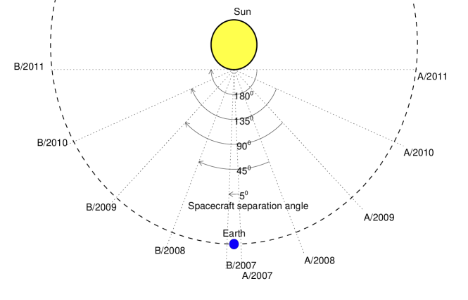
Figure 1.: Schematic figure of the spacecraft orbits of STEREO/A and B relative to Earth, with the spacecraft separation angles $\alpha_{sep}=\alpha_{A}-\alpha_{B}$ indicated approximately at the beginning of the years, ranging from $\approx 5^{\circ}$ in April 2007 to $\approx 180^{\circ}$ in February 2011.

2 OBSERVATIONS AND DATA ANALYSIS

2.1 Observations

We select STEREO observations at spacecraft separation angles with increments of $\approx 45^{\circ}$ over the range of $\alpha_{sep}\approx 0^{\circ}$ to $\approx 180^{\circ}$, which corresponds to time intervals of about a year during the past mission lifetime 2007–2011. A geometric sketch of the spacecraft positions STEREO/A+B relative to the Earth-Sun axis is shown in Fig. 1. Additional constraints in the selection are: (i) The presence of a relatively large prominent active region; (ii) a position in the field-of-view of both spacecraft (since the mutual coverage overlap drops progressively from $180^{\circ}$ initially to $0^{\circ}$ during the first 4 years of the mission); (iii) a time near the central meridian passage of an active region viewed from Earth (to minimize confusion by foreshortening); and (iii) the availability of both STEREO/EUVI/A+B and calibrated SOHO/MDI data. The selection of 5 datasets is listed in Table 1, which includes the following active regions: (1) NOAA 10953 observed on 2007 April 30 (also described in DeRosa et al. 2009; Sandman et al. 2009, Aschwanden and Sandman 2010; Sandman and Aschwanden 2011, Aschwanden et al. 2012), (2) NOAA region 10978 observed on 2007 December 11 (also described in Aschwanden and Sandman 2010, Aschwanden et al. 2012, and subject to an ongoing study by Alex Engell and Aad Van Ballegooijen, private communication), (3) NOAA 11010 observed on 2009 Jan 12, (4) NOAA 11032 observed on 2009 Nov 21, and (5) NOAA 11127 observed on 2010 Nov 23. This selection covers spacecraft separation angles of $\alpha_{sep}\approx 6^{\circ},43^{\circ},89^{\circ},127^{\circ}$, and $170^{\circ}$.

For each of the 5 datasets we stacked the images during a time interval of 20–30 minutes in order to increase the signal-to-noise ratio of the EUVI images. During the first 3 years (2006-2008) the nominal cadence of 171 Å images was 150 s, which yields 8 stacked images per 20 minute interval. Later in the mission, the highest cadence was chosen for the 195 Å wavelength, but dropped from 150 s to 300 s due to the reduced telemetry rate at larger spacecraft distances, which yields 6–12 stacked images per 30 minute interval. In one case (2010 Nov 23) the cadence in EUVI/A and B are not equal, either due to data loss or different telemetry priorities (see time intervals and number of stacked images in Table 1). The solar rotation during the time interval of stacked image sequences was removed to first order by shifting the images by an amount corresponding to the rotation rate at the extracted subimage centers.

Table 1.: Data selection of 5 active regions observed with STEREO/EUVI and SOHO/MDI.

Active	Observing	Observing	Wave-	Number of	Spacecraft
Region	date	times	length	stacked images	separation
		(UT)	(A)	$N_{A}$, $N_{B}$	angle (deg)
10953 (E23S10)	2007-Apr-30	23:00-23:20	171	8, 8	6.1∘
10978 (E14S01)	2007-Dec-11	16:30-16:50	171	8, 8	42.7∘
11010 (E05N18)	2009-Jan-12	00:30-01:00	171	6, 6	89.3∘
11032 (W03N16)	2009-Nov-21	00:30-01:00	195	12, 12	126.9∘
11127 (W08N25)	2010-Nov-23	00:30-01:00	195	12, 6	169.4∘

2.2 Stereoscopic Triangulation

The geometric principles of stereoscopic triangulation are described in Aschwanden et al. (2008; Sections 3.1 and 3.2 therein) for the general case of different spacecraft distances $d_{A}$ and $d_{B}$ from the Sun. The given formulas work correctly up to spacecraft separation angles of $\alpha_{sep}\lower 1.72218pt\hbox{$\;\buildrel<\over{\scriptstyle\sim}\;$}90^{\circ}$, but there is a sign ambiguity for larger separation angles. However, using the publicly available SSW/IDL software in the framework of the Wold Coordinate System (WCS) (Thompson 2006), we can transform a pair of STEREO/A+B images into epipolar coordinates (Inhester 2006), by coaligning to the same Sun center position, derotating the spacecraft roll angles, and rescaling to the same solar distance $d_{A}$), where stereoscopic triangulation is most straightforward. If $(x_{A},y_{A})$ are the cartesian coordinates of a loop position in a STEREO/A image (in units of solar radii measured from Sun center), the relationship between the heliocentric longitudes $(l_{A},l_{B})$ and latitudes $(b_{A},b_{B})$ in the images $A$ and $B$, and the cartesian coordinates $(x_{B},y_{B})$ in the image $B$ are (in the far-field approximation),

$$\begin{array}[]{ll}b_{A}&=\arcsin{(y_{A}/r)}\\ l_{A}&=\arcsin{[x_{A}/(r\ \cos{b_{A}})]}\\ l_{B}&=l_{A}+\alpha_{sep}\\ b_{B}&=b_{A}\\ x_{B}&=r\ \sin(l_{B})\cos(b_{B})\\ y_{B}&=y_{A}\end{array}\ .$$ (1)

where $r=1+h$ is the stereoscopically triangulated distance from Sun center (in units of solar radii). The conversion of image $A$ pixel coordinates $(i_{A},j_{A})$ into dimensionless Sun center coordinates $(x_{A},y_{A})$ is, with $r_{pix}$ the solar radius in units of EUVI pixels sizes,

$$\begin{array}[]{ll}x_{A}&=(i_{A}-i_{0})/r_{pix}\\ y_{A}&=(j_{A}-j_{0})/r_{pix}\end{array}\ ,$$ (2)

and the back-transformation into image $B$ pixel coordinates is,

$$\begin{array}[]{ll}i_{B}&=i_{0}+x_{B}\ r_{pix}\\ j_{B}&=j_{0}+y_{B}\ r_{pix}\end{array}\ ,$$ (3)

where $(i_{0},j_{0})$ are the pixel coordinates of the Sun center in the co-registered epipolar STEREO image pair. There is no sign ambiguity in the coordinate transformation, as long as the triangulated feature is in front of the visible hemisphere (and plane-of-sky through Sun center) for each spacecraft, or more specifically, if the triangulated positions have positive values $z_{A}>0$ and $z_{B}>0$ in each spacecraft coordinate system.

2.3 Magnetic Field Models

Since the two STEREO/A+B spacecraft have an almost symmetric separation angle in east and west direction with respect to Earth, their overlapping field-of-view is always centered closely to the Sun’s central meridian for spacecraft separation angles of $\alpha_{sep}\leq 180^{\circ}$, and thus we have always also a magnetogram from an Earth-bound satellite available, such as from SOHO/MDI, during the considered time period of 2006-2011. We make use of the Michelson Doppler Imager (MDI) daily magnetic field synoptic full-disk data, which are taken every 96 minutes, and thus are near-simultaneous with the STEREO/EUVI images within $\approx 1$ hour. The maximum magnetic field strengths of the 5 analyzed active regions are listed in Table 2, reaching up $B\approx 3100$ G.

We calculate a magnetic potential-field model of each analyzed active region by the method of buried unipolar magnetic charges, which is described to first approximation in Aschwanden and Sandman (2010), and with a higher accuracy including the curvature of the solar surface in Aschwanden et al. (2012). Essentially, a line-of-sight magnetogram $B_{z}(x,y)$ is decomposed into a number (typically $n_{c}=200$) components of buried magnetic charges, each one parameterized with 4 parameters ($B_{j},x_{j},y_{i},z_{j})$ that characterize the surface field strength $B_{j}$ and the 3D position of the magnetic charge below the photospheric surface. The coronal potential field ${\bf B}({\bf x})$ is calculated from the superposition of all $N_{m}$ magnetic charges,

$${\bf B}({\bf x})=\sum_{j=1}^{N_{m}}{\bf B}_{j}({\bf x})=\sum_{j=1}^{N_{m}}B_{j}\left({d_{j}\over r}\right)^{2}{{\bf r}\over r}\ ,$$ (4)

with ${\bf r}=[(x-x_{j}),(y-y_{j}),(z-z_{j})]$ being the distance of a coronal position $[x,y,z]$ from the magnetic charge $j$, ${\bf r}_{j}=(x_{j},y_{j},z_{j})$ is the subphotospheric position of the buried charge, and $d_{j}=\sqrt{1-x_{j}^{2}-y_{j}^{2}-z_{j}^{2}}$ is the depth of the magnetic charge.

We calculate magnetic field lines by starting at photospheric footpoints and extrapolating along the local magnetic field vector ${\bf B}({\bf x})=(B_{x},B_{y},B_{z})$ in steps of $\Delta s=0.004$ solar radii. We initiate the field line footpoints in a regular grid (of say $50\times 50$) footpoints positions, but plot only those field lines that have a photospheric field strength above some threshold, say $B\geq 100$ G.

For the first three active regions where we have sufficient constraints by stereoscopic loops ($N_{loops}\lower 1.72218pt\hbox{$\;\buildrel>\over{\scriptstyle\sim}\;$}20$), we calculate also a nonlinear force-free field (NLFFF) solution according to a new code based on an analytical approximation of divergence-free and force-free fields that includes an azimuthal magnetic field component with vertical twist and is accurate to second-order (of the force-free parameter $\alpha$). This new NLFFF code uses the constraints of a line-for-sight magnetogram to define the potential field (Eq. 4) and is suitable for fast forward-fitting to coronal field constraints, such as the stereoscopically triangulated 3D loop coordinates as calculated here. The analytical theory of this new NLFFF code is described in Aschwanden (2012), the numerical code and tests in Aschwanden and Malanushenko (2012), and first solar applications to four stereoscopically observed active regions in Aschwanden et al. (2012).

2.4 Data Analysis and Results

In Figs. 2–6 we present the results of stereoscopically triangulated loops for the 5 analyzed active regions and compare them with magnetic potential field and force-free field models. In each of the Figures we use the following layout of panels: Partial STEREO/A and B images are shown in the top panels, each one with a field-of-view that encompasses the active region of interest. The STEREO/A and B images are shown for the brightness on a logarithmic color scale (top panels), as well as in a highpass-filtered version (by unsharp masking, i.e., by subtracting a $3\times 3$ boxcar-smoothed image from the original image) to enhance the loop structures (panels in second row). The SOHO/MDI magnetogram is shown in the bottom right panel, which has a different field-of-view from an Earth-bound vantage point. In addition we show a side view of the active region by rotating the magnetogram view by $90^{\circ}$ to the north (bottom left panel). In all panels, the projections of stereoscopically triangulated loops are shown in blue color, and the magnetic potential field lines in red color.

Table 2.: Data analysis of selection 5 active regions.

Active	Number	Misalignment	Misalignment	Stereoscopy	Magnetic
Region	of	angle	angle	error	field strength
	loops	$\mu_{PF}$ (deg)	$\mu_{FFF}$ (deg)	$\mu_{SE}$ (deg)	B(Gauss)
10953	100	27.7∘	$19.8^{\circ}$	9.4∘	[-3134,+1425]
10978	52	20.8∘	$15.1^{\circ}$	8.9∘	[-2270,+2037]
11007	20	36.2∘	$16.5^{\circ}$	…	[ -737,+1342]
11035	15	29.8∘	$17.4^{\circ}$	…	[ -997, +774]
11161	5	39.4∘	$21.2^{\circ}$	…	[-2033, +884]

The first case is active region NOAA 10953 (Fig. 2), where we display the same 100 loop segments that have been triangulated in an earlier study (Aschwanden and Sandman 2010). The spacecraft separation angle is $\alpha_{sep}=6.1^{\circ}$ and the almost identical direction of the line-of-sights of both STEREO/A and B spacecraft makes it easy to identify the corresponding loops in A and B, and thus the triangulation is very reliable. Note that the height range where discernable loops can be traced in the highpass-filtered images is about $h_{max}\approx 0.1$ solar radii (or $\approx 70$ Mm), which is commensurable with the hydrostatic density scale height expected for a temperature of $T=1.0$ MK that corresponds to the peak sensitivity of the EUVI 171 Å filter. This is particularly well seen in the side view shown in the bottom left panel in Fig. 2. A measurement of the mean misalignment angle averaged over 10 positions of the 100 reconstructed loops with the local magnetic potential field shows a value of $\mu_{PF}=27.7^{\circ}$ (Table 2), similar to earlier work (Aschwanden and Sandman 2010; Sandman and Aschwanden 2011). However, forward-fitting of a nonlinear force-free field model reduces the misalignment to $\mu_{FFF}=19.8^{\circ}$, which implies that this active region is slightly nonpotential. The remaining misalignment is attributed to at least two reasons, partially to inadequate parameterization of the force-free field model, and partially to stereoscopic measurement errors $\alpha_{SE}$ due to misidentified loop correspondences and limited spatial resolution. An empirical estimate of the stereoscopic error was devised in Aschwanden and Sandman (2010), based on the statistical non-parallelity of closely-spaced triangulated loop 3D trajectories, which yielded for this case a value of $\alpha_{SE}=9.4^{\circ}$. In summary, we find that this active region is very suitable for stereoscopy, allows to discern a large number (100) of loops, minimizes the stereoscopic correspondence problem due to the small ($\alpha_{sep}=6.1^{\circ}$) spacecraft separation angle, displays a moderate misalignment angle and stereoscopic measurement error ($\mu_{SE}=9.4^{\circ}$). This well-defined case will serve as a reference for stereoscopy at larger angles.

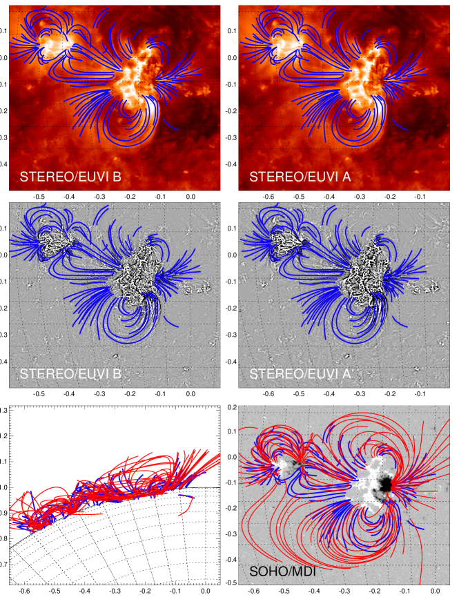
Figure 2.: STEREO/EUVI spacecraft A (top right) and spacecraft B image (top left), of active region AR 10953, observed on 2007 Apr 30, 23:00 UT in the 171 Å wavelength, with a spacecraft separation angle of $\alpha_{sep}=6.1^{\circ}$. The images are highpass-filtered to enhance loop structures (middle left and right panels). A near-simultaneous SOHO/MDI magnetogram is shown (bottom right), overlaid with the stereoscopically triangulated loops (blue curves) and magnetic field lines computed with a nonlinear force-free model (red curves), viewed from the direction of Earth or SOHO/MDI (bottom right), and rotated by $90^{0}$ to the north (bottom left).

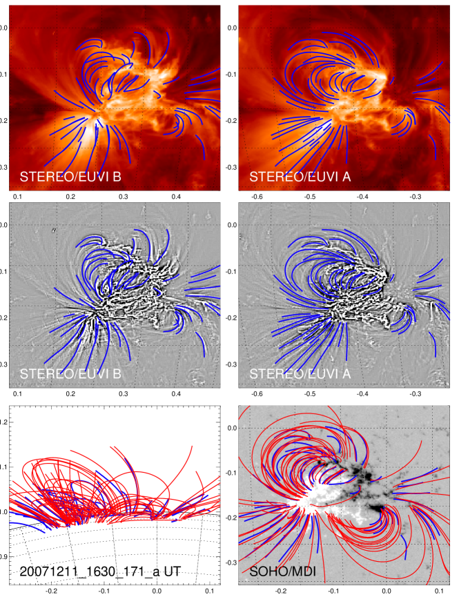
Figure 3.: Active region AR 10978, observed on 2007 Dec 11, 16:30 UT in the 171 Å wavelength, with a spacecraft separation angle of $\alpha_{sep}=42.7^{\circ}$. A SOHO/MDI magnetogram is shown (bottom right), overlaid with the stereoscopically triangulated loops (blue curves) and magnetic field lines computed with a nonlinear force-free model (red curves).

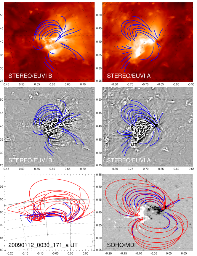
Figure 4.: Active region AR 11010, observed on 2009 Jan 12, 00:30 UT in the 171 Å wavelength, with a spacecraft separation angle of $\alpha_{sep}=89.3^{\circ}$. A SOHO/MDI magnetogram is shown (bottom right), overlaid with the stereoscopically triangulated loops (blue curves) and magnetic field lines computed with a nonlinear force-free model (red curves).

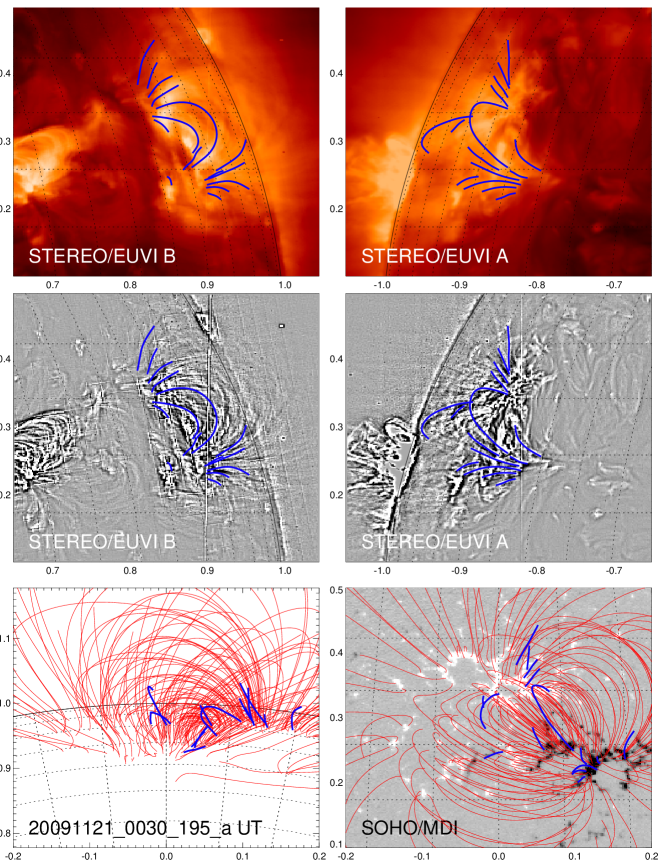
Figure 5.: Active region AR 11032, observed on 2009 Nov 21, 00:30 UT in the 195 Å wavelength, with a spacecraft separation angle of $\alpha_{sep}=126.9^{\circ}$. A SOHO/MDI magnetogram is shown, overlaid with the stereoscopically triangulated loops (blue curves) and magnetic field lines computed with a potential field model. Magnetic field lines have a footpoint threshold of $B>100$ G.

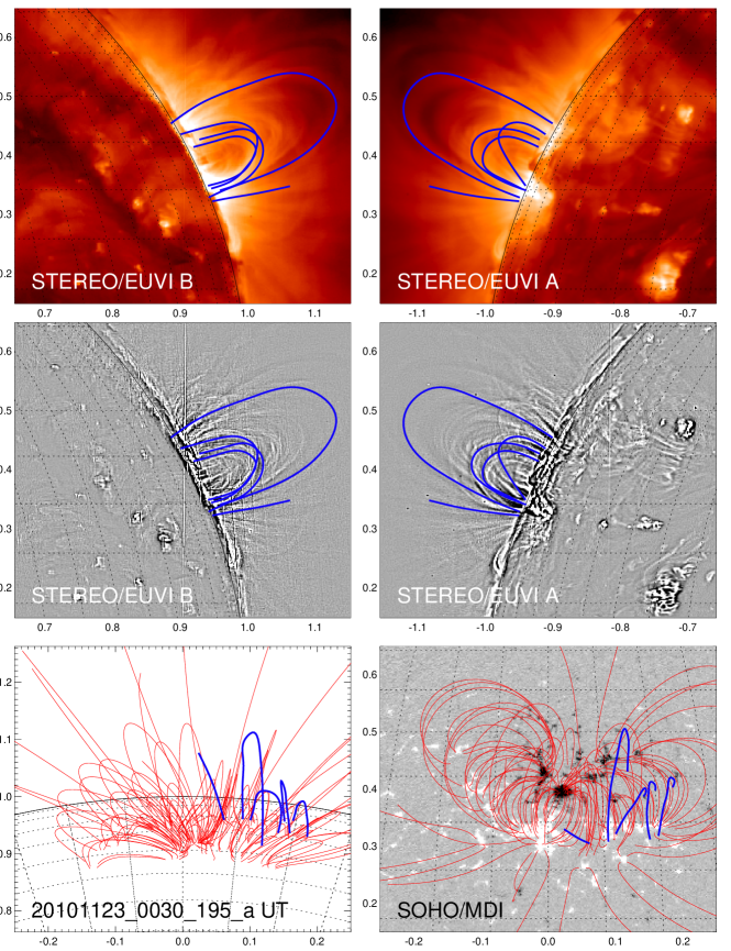
Figure 6.: Active region AR 11127, observed on 2010 Nov 23, 00:30 UT in the 195 Å wavelength, with a spacecraft separation angle of $\alpha_{sep}=169.4^{\circ}$. A SOHO/MDI magnetogram is shown, overlaid with the stereoscopically triangulated loops (blue curves) and magnetic field lines computed with a potential field model. Magnetic field lines have a footpoint threshold of $B>100$ G.

The second case is active region NOAA 10978 (Fig. 3), observed on 2007 Dec 11 with a spacecraft separation angle of $\alpha_{sep}=42.7^{\circ}$. Note that the views from EUVI/A and B appear already to be significantly different with regard to the orientation of the triangulated loops, as seen from a distinctly different aspect angle. A set of 52 coronal loops were stereoscopically triangulated in this region (Aschwanden and Sandman 2010), a mean misalignment angle of $\mu_{PF}=20.8^{\circ}$ is found for a potential field model, and a reduced value of $\mu_{FFF}=15.1^{\circ}$ is found for the force-free model (Table 2), while a stereoscopic error of $\alpha_{SE}=8.9^{\circ}$ is estimated (Aschwanden and Sandman 2010). Thus, the quality of stereoscopic triangulation (as well as the degree of non-potentiality) is similar to the first active region, although we performed stereoscopy with a 7 times larger spacecraft separation angle ($\alpha_{sep}=42.7^{\circ}$) than before ($\alpha_{sep}=6.1^{\circ}$). Apparently, stereoscopy is still easy at such angles, partially helped by the fact that the active region is located near the central meridian ($\pm 20^{\circ}$) for both spacecraft, which provides an unobstructed view from top down, so that the peripheral loops of the active region do not overarch the core of the active region, where the bright reticulated moss pattern (Berger et al. 1999) makes it almost impossible to discern faint loops in the highpass-filtered images. The top-down view provides also an optimum aspect angle to disentangle closely-spaced loops, which is an important criterion in the stereosopic correspondence identification.

The third case is active region NOAA 11010 (Fig. 4), observed on 2009 Jan 12 with a near-orthogonal spacecraft separation angle of $\alpha_{sep}=89.3^{\circ}$. Due to the quadrature of the spacecraft, only a sector of $\pm 45^{\circ}$ east and west of the central meridian (viewed from Earth) is jointly visible by both spacecraft. This particular active region is seen at a $45^{\circ}$ angle by both STEREO/A and STEREO/B. This symmetric view is the optimum condition to discern a large number of inclined loop segments and to identify the stereoscopic correspondence. We triangulate some 20 loop segments, which appear almost mirrored in the STEREO/A and B image due to the east-west symmetry of the magnetic dipole. A mean misalignment angle of $\mu_{PF}=36.2^{\circ}$ with the potential field model is found, and a reduced value of $\mu_{FFF}=16.5^{\circ}$ with the force-free field model. An estimate of the statistical (non-parallelity) stereoscopic error is not possible due to the small number of triangulated loops. Thus, we conclude that stereoscopy is still possible in quadrature. Mathematically, the orthogonal projections should yield the most accurate 3D coordinates of a curvi-linear structure, but in practice, confusion of multiple structures with near-aligned projections can cause a disentangling problem in the stereoscopic correspondence identification at this intermediate angle.

The fourth case is active region NOAA 11032 (Fig. 5), observed on 2009 Nov 21 with a large spacecraft separation angle of $\alpha_{sep}=126.9^{\circ}$. STEREO/A sees the active region near the east limb from an almost side-on perspective, while STEREO/B sees a similar mirror image near the west limb, where confusion near the limb makes the stereoscopic correspondence identification more difficult. We trace some 15 loop segments, but do not succeed in pinning down a larger number of loops, partially because this active region is small and does not exhibit numerous bright loops, and partially because of increasing confusion problems near the limb. We searched for larger active regions over several months around this time, but were not successful due to a dearth of solar activity during this time. We find a misalignment angle of $\mu_{PF}=29.8^{\circ}$ for the potential field, and $\mu_{FFF}=17.4^{\circ}$ for the force-free field model, which is still comparable with the previous active regions triangulated at smaller sterescopic angles. Thus, stereoscopy seems to be still feasible at such large stereoscopic angles.

The last case is active region NOAA 11127 (Fig. 6), observed on 2010 Nov 23 with a very large spacecraft separation angle of $\alpha_{sep}=169.4^{\circ}$, only two months before the two STEREO spacecraft pass the largest separation point. At this point, the common field-of-view that is overlapping from STEREO/A and B is only the central meridian zone seen from Earth (or the opposite meridian behind the Sun). STEREO/A observes active region NOAA 11127 at its east limb, while STEREO/B sees it at its west limb, so both spacecraft see only the vertical structure of the active region from a side view (see Fig. 6 top). This particular configuration is very unfavorable for stereoscopy. Although the vertical structure in altitude can be measured very accurately, the uncertainty in horizontal direction in longitude is very large and suffers moreover the sign ambiguity of positive or negative longitude difference with respect to the limb seen from Earth. Consequently, we have reliable information on the altitude and latitude of loops, while the longitude is essentially ill-defined. In order to reduce the large scatter in the measurement of $z$-coordinates along a loop, introduced by the near-infinite amplification of parallax uncertainties tangentially at the limb, we restrict the general solution of geometric 3D triangulation to planar loops, by applying a linear regression fit of the $z(y)$ coordinates. The example in Fig. 6 shows that we can trace some (5) loops in the plane of the sky and have no problem in identifying the stereoscopic counterparts in both STEREO/A and B images, but the stereoscopic triangulation is ill-defined at this singularity of the sign change in the parallax effect. The misalignment between the three loop directions and the potential field is $\mu_{PF}=39.4^{\circ}$, and for the force-free field model is $\mu_{FFF}=21.2^{\circ}$, which indicates that the orientation of the loop planes is less reliably determined. Stereoscopic triangulation brakes down at this singularity of separation angles at $\alpha_{sep}\approx 180^{\circ}$, although the stereoscopic correspondence problem is very much reduced for the “mirror images”, similar to the near-identical images at small separation angles $\alpha_{sep}\lower 1.72218pt\hbox{$\;\buildrel>\over{\scriptstyle\sim}\;$}0^{\circ}$.

3 DISCUSSION

We are discussing now the pro’s and con’s of stereoscopy at small and large aspect angles, which includes quantitative estimates of the formal error of stereoscopic triangulation (Section 3.1), the stereoscopic correspondence and confusion problem (Section 3.2), and the statistical probability of stereoscopable active regions during the full duration of the STEREO mission (Section 3.3), all as a function of the stereoscopic aspect angle (or spacecraft separation angle $\alpha_{sep}$ in the case of the STEREO mission).

3.1 Stereoscopic Triangulation Error

Stereoscopic triangulation involves a parallax angle around the normal of the epipolar plane. For the STEREO mission, the epipolar plane intersects the Sun center and the two spacecraft A and B positions, which are separated mostly in east-west direction. No parallax effect occurs when the loop axis coincides with the epipolar plane, i.e., when the loop axis points in east-west direction. Thus, the accuracy of stereoscopic triangulation depends most sensitively on this orientation angle $\vartheta$, which we define as the angle between the loop direction and the normal of the epipolar plane (i.e., approximately the y-axis of a solar image in north-south direction). If the position of a loop centroid can be determined with an accuracy of a half pixel size $\Delta_{pix}/2$, the dependence of the stereoscopic error on the orientation angle $\vartheta$ is then (Aschwanden et al. 2008),

$$\sigma(\vartheta)={\Delta_{pix}\over 2}\sqrt{1+\tan^{2}(\vartheta)}={\Delta_{pix}\over 2}{1\over\cos(\vartheta)}\ .$$ (5)

Thus, for a highly inclined loop that has an eastern and western footpoint at the same latitude, the stereoscopic error is minimal near the loop footpoints (pointing in north-south direction) and at maximum near the loop apex (pointing in east-west direction).

In addition, the accuracy of stereoscopic triangulation depends also on the aspect angle (or spacecraft separation angle $\alpha_{sep}$), which can be quantified with an error trapezoid as shown in Fig. 7. If the half separation angle $\alpha_{sep}/2$ is defined symmetrically to the Earth-Sun axis (z-axis), the uncertainty in z-direction is $\sigma_{z}=(\Delta_{pix}/2)/\sin(\alpha_{sep}/2)$ and is in the x-direction (in the epipolar plane) $\sigma_{x}=(\Delta_{pix}/2)/\sin([\pi-\alpha_{sep}]/2)$. Including also a half pixel-size error $\sigma_{y}=(\Delta_{pix}/2)$ in the y-direction, we have then a combined error for the 3D position of a triangulated point as,

$$\sigma(\alpha_{sep})=\sqrt{\sigma_{x}^{2}+\sigma_{y}^{2}+\sigma_{z}^{2}}={\Delta_{pix}\over 2}\sqrt{1+{1\over\sin^{2}({\alpha_{sep}/2})}+{1\over\sin^{2}{[(\pi-\alpha_{sep})/2]}}}\ .$$ (6)

This positional error is symmetric for small $\alpha_{sep}$ and large stereoscopic angles $(\pi-\alpha_{sep})$, and has a minimum at an orthogonal angle of $\alpha_{sep}=\pi/2$. The error is largest in z-direction for small spacecraft separation angles, while it is largest in x-direction for separation angles near $\alpha_{sep}\lower 1.72218pt\hbox{$\;\buildrel<\over{\scriptstyle\sim}\;$}180^{\circ}$.

Figure 7.: The error trapezoid of stereoscopic triangulation is shown (grey area), given by the two line-of-sights of the two observer directions A and B, separated by an angle $\alpha_{sep}$. The uncertainties $\Delta x$ in x-direction and spacecraft in z-direction depend on the pixel width $\Delta_{pix}$ and half aspect angle $\alpha_{sep}/2$.

To compare the relative importance of the two discussed sources of errors we can evaluate the parameters that increase the individual errors by a factor of two. This is obtained when the orientation angle of a loop segment (with respect to the east-west direction) increases from $\vartheta=0^{\circ}$ to $\vartheta\approx 60^{\circ}$, or if the spacecraft separation angle changes from the optimum angle $\alpha_{sep}=90^{\circ}$ to $\alpha_{sep}=25^{\circ}$ (or $\alpha_{sep}=155^{\circ}$, respectively). If stereoscopy at small angles of $\alpha_{sep}=5^{\circ}$ is attempted, the positional error is about ten-fold (corresponding to $\approx 8\Delta_{pix}$), compared with the optimum angle at $\alpha_{sep}=90^{\circ}$ (corresponding to $\approx 0.8\Delta_{pix}$). For STEREO/EUVI with a pixel size of $\Delta_{pix}=1.6\hbox{${}^{\prime\prime}$}\approx 1.2$ Mm, this amounts to an accuracy range of $\approx 1-10$ Mm.

3.2 Stereoscopic Correspondence and Confusion Error

The previous considerations are valid for isolated loops that can be unambiguously disentangled in an active region, in both the STEREO/A and B images. However, this is rarely the case. In crowded parts of active regions, the correspondence of a particular loop in image A with the identical loop in image B can often not properly be identified. We call this confusion problem also the stereoscopic correspondence problem, which appears in every stereoscopic tie-point triangulation method. In order to quantify this source of error, we have to consider the area density of loops and their relative orientation. A top-down view of an active region, e.g., as seen for small stereoscopic angles by both spacecraft for an active region near disk center (e.g., Fig. 2), generally allows a better separation of individual loops, because only the lowest density scale height is detected (due to hydrostatic gravitational stratification), and neighbored loop segments do not obstruct each other due to the foreshortening projection effect near the footpoints. In contrast, every active region seen near the limb, shows many loops at different longitudes, but at similar latitudes, cospatially on top of each other, which represents the most severe confusion problem. Thus, we can essentially quantify the degree of confusion by the loop number density per pixel, which approximately scales with the inverse cosine-function of the center-to-limb angle due to foreshortening. In other words, we can define a quality factor $C(\rho)$ for identifying the stereoscopic correspondence $C$ of properly disentangled coronal loops, which drops from $C(\rho=0)=1$ at disk center to $C(\rho=\pi/2)=0$ at the limb, where $\rho$ is the center-to-limb angle measured from Sun center,

$$C(\rho)=|\cos(\rho)|\qquad 0\leq|\rho|\leq\pi/2\ .$$ (7)

Figure 8.: Quality factor $Q$ of stereoscopic triangulation as a function of the spacecraft separation angle $\alpha_{sep}$, which is a function of the accuracy $A$ of triangulated stereoscopic positions and the stereoscopic correspondence quality factor $C$. The best quality (within a factor of 2) occurs in the range of $\alpha_{sep}=22^{\circ}-125^{\circ}$.

The orbits of the STEREO mission reduce the overlapping area on the solar surface that can be jointly viewed by both spacecraft A and B linearly with increasing spacecraft separation angle, so that the center-to-limb distance $\rho$ of an active region located on the central meridian (viewed from Earth) is related to the spacecraft separation angle by

$$\rho={\alpha_{sep}\over 2}\ ,$$ (8)

increasing linearly with the separation angle from $\rho=0$ at the beginning of the mission to $\rho=\pi/2$ at maximum spacecraft separation angle. The location of an active region at the central meridian provides the best view for both spacecraft, because an asymmetric location would move the active region closer to the limb for one of the spacecraft, and thus would increase the degree of confusion, as we verified by triangulating a number of asymmetric cases. Thus, we can express the quality factor of stereoscopic correspondence $C$ (Eq. 7) by the spacecraft separation angle (Eq. 8) and obtain the relationship,

$$C(\alpha_{sep})=\cos(\alpha_{sep}/2)\qquad 0\leq\alpha_{sep}\leq\pi\ .$$ (9)

Defining a quality factor $Q$ for stereoscopic triangulation by combining the stereoscopic correspondence quality $C$ (Eq. 9) with the accuracy $A$ of stereoscopic positions (Eq. 6), which we may define by the normalized inverse error (i.e., $A=\sigma(\alpha_{sep,min})/\sigma(\alpha_{sep})$), we obtain

$$Q(\alpha_{sep})=C\times A={\sqrt{3}\ \cos{(\alpha_{sep}/2)}\over\sqrt{1+{1/\sin^{2}{(\alpha_{sep}/2)}}+{1/\sin^{2}{[(\pi-\alpha_{sep})/2}]}}}\ .$$ (10)

We plot the functional dependence of this stereoscopic quality factor $Q(\alpha_{sep})$ together with their underlying factors $A(\alpha_{sep})$ and $C(\alpha_{sep})$ in Fig. 8 and obtain now an asymmetric function of time (or spacecraft separation angle) that favors smaller stereoscopic angles. The stereoscopic quality factor is most favorable (within a factor of 2) in the range of $\alpha_{sep}=22^{\circ}-125^{\circ}$, which corresponds to the mission phase between August 2007 and November 2009. The same optimum range will repeat again at the backside of the Sun 5 years later between August 2012 and November 2014.

From our analysis of 5 active regions spread over the entire spacecraft separation angle range we find acceptable results regarding triangulation accuracy in the range of separation angles of $\alpha_{sep}=6^{\circ}$ and $127^{\circ}$ (based on acceptable misalignment angles of $\alpha_{PF}\lower 1.72218pt\hbox{$\;\buildrel<\over{\scriptstyle\sim}\;$}35^{\circ}$, which coincides with the predicted optimum range of $\alpha_{sep}\approx 22^{\circ}-125^{\circ}$, while stereoscopy definitely brakes down at $\alpha_{sep}\lower 1.72218pt\hbox{$\;\buildrel<\over{\scriptstyle\sim}\;$}170^{\circ}$, as predicted by theory (Fig. 8 and Eq. 10).

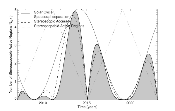
Figure 9.: The statistically expected variation of the number of active regions $N(t)$ during the solar cycle (thin solid curve), the spacecraft separation angle $\alpha_{sep}(t)$ (dotted curve), the stereoscopic accuracy $A(t)$ (dashed curve), and the expected number of stereoscopable active regions $N_{AR}(t)$ (curve with grey area) as a function of time during a full 16-year mission cycle of the STEREO mission.

3.3 The Statistical Probability of Stereoscopy

There are different factors that affect the quality or feasibility of solar stereoscopy, such as (i) the availability of large active regions (which varies statistically as a function of solar cycle), (ii) the simultaneous viewing by both spacecraft STEREO/A and B (which depends on the spacecraft separation angle), (iii) the geometric foreshortening that affects the stereoscopic correspondence problem (which depends on the center-to-limb distance for each spacecraft view), and (iv) the time of the central meridian passage of the active region for a viewer from Earth (which determines the symmetry of views for both spacecraft, where minimum confusion occurs in the stereoscopic correspondence identification). All but the first factor depend on the spacecraft separation angle $\alpha_{sep}(t)$, which is a specific function of time for the STEREO mission (with a complete cycle of 16 years). In order to assess the science return of the STEREO mission or future missions with stereoscopic capabilities, it is instructive to quantify the statistical probability of acceptable stereoscopic results as a function of spacecraft separation angle or time.

We already quantified the quality of stereoscopy $Q(\alpha_{sep})$ as a function of the stereoscopic angle in Eq. (10). Let us define the number probability $N(t)$ of existing active regions at a given time $t$ with a squared sinusoidal modulation during the solar cycle,

$$N(t)=N_{0}\ \sin{\left({\pi(t-t_{0})\over T_{cycle}}\right)}\ ,$$ (11)

where $N_{0}\approx 10$ is the maximum number of active regions existing on the total solar surface during the maximum of the solar cycle, $t_{0}$ is the time of the solar minimum (e.g., $t_{min}\approx 2009$), and $T_{cycle}\approx 10.3$ yrs the current average solar cycle length.

The second effect is the overlapping area on the solar surface that is simultaneously seen by both spacecraft STEREO/A and B, which decreases linearly with the spacecraft separation angle from 50% at $\alpha_{sep}(t=t_{1})$ (with $t_{1}=2007.1$ at the start of spacecraft separation) to 0% at $\alpha_{sep}(t=t_{2})$ (with $t_{2}=2011.1$ at maximum separation), and then increases linearly again for the next quarter phase of a mission cycle. If we fold the variation $N(t)$ of the solar cycle (Eq. 11) with the triangular stereoscopic overlap area variation $A(t)$ together, we obtain a statistical probability for the number of stereoscopically triangulable active regions. However, the number of accurate stereoscopical triangulations scales with the quality factor $Q(\alpha_{sep})$ (Eq. 10), where the spacecraft separation angle $\alpha_{sep}(t)$ is a piece-wise linear (triangular) function of time $t$ according to the spacecraft orbit. Essentially we are assuming that the probability of successfull stereoscopic triangulations at a given time scales with the quality factor or feasibility of accurate stereoscopy at this time. So, we obtain a combined probability of stereoscopically triangulable active regions of,

$$N_{AR}(t)=N(t)\times Q[\alpha_{sep}(t)]\ .$$ (12)

In Fig. 9 we show this combined statistical probability of feasible stereoscopy in terms of the expected number of active regions for a full mission cycle of 16 years, from 2006 to 2022. It shows that the best periods for solar stereoscopy are during 2012-2014, 2016-2017, and 2021-2023.

4 CONCLUSIONS

After the STEREO mission reached for the first time a full $360^{\circ}$ view of the Sun this year (2007 Feb 6), the two STEREO A and B spacecraft covered also for the first time the complete range of stereoscopic viewing angles from $\alpha_{sep}\lower 1.72218pt\hbox{$\;\buildrel>\over{\scriptstyle\sim}\;$}0^{\circ}$ to $\alpha_{sep}\lower 1.72218pt\hbox{$\;\buildrel<\over{\scriptstyle\sim}\;$}180^{\circ}$. We explored the feasibility of stereoscopic triangulation for coronal loops in the entire angular range by selecting 5 datasets with viewing angles at $\alpha_{sep}\approx 6^{\circ},43^{\circ},89^{\circ},127^{\circ}$ and $169^{\circ}$. Because previous efforts for solar stereoscopy covered only a range of small stereoscopic angles ($\alpha_{sep}\lower 1.72218pt\hbox{$\;\buildrel<\over{\scriptstyle\sim}\;$}45^{\circ}$), we had to generalize the stereoscopic triangulation code for large angles up to $\alpha_{sep}\leq 180^{\circ}$. We find that stereoscopy of coronal loops is feasible with good accuracy for cases in the range $\alpha_{sep}\approx 6^{\circ}-127^{\circ}$, a range that is also theoretically predicted by taking into account the triangulation errors due to finite spatial resolution and confusion in the stereoscopic correspondence identification in image pairs, which is hampered by projection effects and foreshortening for viewing angles near the limb. Accurate stereoscopy (within a factor of 2 of the best possible accuracy) is predicted for a spacecraft separation angle range of $\alpha_{sep}\approx 22^{\circ}-125^{\circ}$. Based on this model we predict that the best periods for stereoscopic 3D reconstruction during a full 16-year STREREO mission cycle occur during 2012-2014, 2016-2017, and 2021-2023, taking the variation in the number of active regions during the solar cycle into account also.

Why is the accuracy of stereoscopic 3D reconstruction so important? Solar stereoscopy has the potential to quantify the coronal magnetic field independently of conventional 2D magnetogram and 3D vector magnetograph extrapolation methods, and thus serves as an important arbiter in testing theoretical models of magnetic potential fields, linear force-free field models (LFFF), and nonlinear force-free field models (NLFFF). A benchmark test of a dozen of NLFFF codes has been compared with stereoscopic 3D reconstruction of coronal loops and a mismatch in the 3D misalignment angle of $\mu\approx 24^{\circ}-44^{\circ}$ has been identified (DeRosa et al. 2009), which is attributed partially to the non-force-freeness of the photospheric magnetic field, and partially to insufficient constraints of the boundary conditions of the extrapolation codes. Empirical estimates of the error of stereoscopic triangulation based on the non-parallelity of loops in close proximity has yielded uncertainties of $\mu_{SE}\approx 7^{\circ}-12^{\circ}$. Thus the residual difference in the misalignment is attributed to either the non-potentiality of the magnetic field (in the case of potential field models), or to the non-force-freeness of the photospheric field (for NLFFF models). We calculated also magnetic potential fields here for all stereoscopically triangulated active regions and found mean misalignment angles of $\mu_{PF}\approx 21^{\circ}-39^{\circ}$, which improved to $\mu_{FFF}\approx 15^{\circ}-21^{\circ}$ for a nonlinear force-free model, which testifies the reliability of stereoscopic reconstruction for the first time over a large angular range. The only case where stereoscopy clearly fails is found for an extremely large separation angle of ($\alpha_{sep}\approx 170^{\circ}$), which is also reflected in the largest deviation of misalignment angles found ($\mu_{NP}\approx 39^{\circ}$, $\mu_{FFF}\approx 21^{\circ}$). Based on these positive results of stereoscopic accuracy over an extended angular range from small to large spacecraft separation angles we anticipate that 3D reconstruction of coronal loops by stereoscopic triangulation will continue to play an important role in testing theoretical magnetic field models for the future phases of the STEREO mission, especially since stereoscopy of a single image pair does not require a high cadence and telemetry rate at large distances behind the Sun.

This work is supported by the NASA STEREO mission under NRL contract N00173-02-C-2035. The STEREO/ SECCHI data used here are produced by an international consortium of the Naval Research Laboratory (USA), Lockheed Martin Solar and Astrophysics Lab (USA), NASA Goddard Space Flight Center (USA), Rutherford Appleton Laboratory (UK), University of Birmingham (UK), Max-Planck-Institut für Sonnensystemforschung (Germany), Centre Spatiale de Liège (Belgium), Institut d’Optique Théorique et Applique (France), Institute d’Astrophysique Spatiale (France). The USA institutions were funded by NASA; the UK institutions by the Science & Technology Facility Council (which used to be the Particle Physics and Astronomy Research Council, PPARC); the German institutions by Deutsches Zentrum für Luft- und Raumfahrt e.V. (DLR); the Belgian institutions by Belgian Science Policy Office; the French institutions by Centre National d’Etudes Spatiales (CNES), and the Centre National de la Recherche Scientifique (CNRS). The NRL effort was also supported by the USAF Space Test Program and the Office of Naval Research.

References

Aschwanden, M.J., Wülser, J.P., Nitta, N., Lemen, J. 2008, Astrophys. J. 679, 827.

Aschwanden, M.J. 2009, Space Science Rev. 149, 31.

Aschwanden, M.J. and Sandman, A.W. 2010, Astronom. J. 140, 723.

Aschwanden, M.J. 2012, Sol.Phys. (subm.), A nonlinear force-free magnetic field approximation suitable for fast forward-fitting to coronal loops. I. Theory, http:www.lmsal.com/~aschwand/eprints/2012˙fff1.pdf

Aschwanden, M.J. and Malanushenko,A. 2012, Sol.Phys. (subm), A nonlinear force-free magnetic field approximation suitable for fast forward-fitting to coronal loops. II. Numeric Code and Tests, http://www.lmsal.com/~aschwand/eprints/2012˙fff2.pdf

Aschwanden, M.J., Wuelser,J.-P., Nitta, N.V., Lemen, J.R., Schrijver, C.J., DeRosa, M., and Malanushenko, A. 2012, ApJ (subm), First 3D Reconstructions of Coronal Loops with the STEREO A and B Spacecraft: IV. Magnetic Field Modeling with Twisted Force-Free Fields, http://www.lmsal.com/~aschwand/eprints/2012˙stereo4.pdf, http://www.lmsal.com/~aschwand/movies/STEREO˙fff˙movies

Bemporad, A. 2009, Astrophys. J. 701, 298.

Berger, T.E., DePontieu, B., Fletcher, L., Schrijver, C.J., Tarbell, T.D., and Title, A.M. 1999, Solar Phys. 190, 409.

DeRosa, M.L., Schrijver, C.J., Barnes, G., Leka, K.D., Lites, B.W., Aschwanden, M.J., Amari, T., Canou, A., McTiernan, J.M., Regnier, S., Thalmann, J., Valori, G., Wheatland, M.S., Wiegelmann, T., Cheung, M.C.M., Conlon, P.A., Fuhrmann, M., Inhester, B., and Tadesse, T. 2009, Astrophys. J. 696, 1780.

Feng, L., Inhester, B., Solanki, S., Wiegelmann, T., Podlipnik, B., Howard, R.A., and Wülser, J.P. 2007, Astrophys. J. 671, L205.

Feng, L., Inhester, B., Solanki, S.K., Wilhelm, K., Wiegelmann, T., Podlipnik, B., Howard, R.A., Plunkett, S.P., Wülser, J.P., and Gan, W.Q. 2009, Astrophys. J. 700, 292.

Howard, R.A., Howard,R.A., Moses, J.D., Vourlidas, A., Newmark, J.S., Socker, D.G., Plunkett, S.P., Korendyke, C.M., Cook, J.W., Hurley, A., Davila, J.M. and 36 co-authors, 2008, Space Science Rev. 136, 67.

Inhester, B. 2006, ArXiv e-print: astro-ph/0612649.

Kaiser, M.L., Kucera, T.A., Davila, J.M., St. Cyr, O.C., Guhathakurta, M., and Christian, E. 2008, Space Science Rev. 136, 5.

Liewer, P.C., DeJong, E.M., Hall, J.R., Howard, R.A., Thompson, W.T., Culhane, J.L., Bone, L., van Driel-Gesztelyi, L. 2009, Solar Phys. 256, 57.

Sandman, A., Aschwanden, M.J., DeRosa, M., Wülser, J.P., and Alexander, D. 2009, Solar Phys. 259, 1.

Sandman, A.W. and Aschwanden, M.J. 2011, Solar Phys. 270, 503.

Thompson, W.T. 2006, Astron. Astrophys. 449, 791.

Thompson, W.T. 2011, J. Atmos. Solar-Terr. Phys. 73, 1138.

Thompson, W.T., Davila, J.M., St. Cyr, O.C., and Reginald, N.L. 2011, Solar Phys. 272, 215.

Wülser, J.P., Lemen, J.R., Tarbell, T.D., Wolfson, C.J., Cannon, J.C., Carpenter, B.A., Duncan, D.W., Gradwohl, G.S., Meyer, S.B., Moore, A.S., and 24 co-authors, 2004, SPIE 5171, 111.