A Nonlinear Force-Free Magnetic Field Approximation Suitable for Fast Forward-Fitting to Coronal Loops. II. Numeric Code and Tests

Abstract

Based on a second-order approximation of nonlinear force-free magnetic field solutions in terms of uniformly twisted field lines derived in Paper I, we develop here a numeric code that is capable to forward-fit such analytical solutions to arbitrary magnetogram (or vector magnetograph) data combined with (stereoscopically triangulated) coronal loop 3D coordinates. We test the code here by forward-fitting to six potential field and six nonpotential field cases simulated with our analytical model, as well as by forward-fitting to an exactly force-free solution of the Low and Lou (1990) model. The forward-fitting tests demonstrate: (i) a satisfactory convergence behavior (with typical misalignment angles of $\mu\approx 1^{\circ}-10^{\circ}$), (ii) relatively fast computation times (from seconds to a few minutes), and (iii) the high fidelity of retrieved force-free $\alpha$-parameters ($\alpha_{\rm fit}/\alpha_{\rm model}\approx 0.9-1.0$ for simulations and $\alpha_{\rm fit}/\alpha_{\rm model}\approx 0.7\pm 0.3$ for the Low and Lou model). The salient feature of this numeric code is the relatively fast computation of a quasi-forcefree magnetic field, which closely matches the geometry of coronal loops in active regions, and complements the existing nonlinear force-free field (NLFFF) codes based on photospheric magnetograms without coronal constraints.

1 Introduction

This paper contains a description of a new numerical code that performs fast forward-fitting of nonlinear force-free magnetic fields (NLFFF). An alternative NLFFF forward-fitting code has been pioneered by Malanushenko et al.(2009), which first fits separate linear force-free solutions to individual loops, and in a next step retrieves a self-consistent NLFFF solution from the obtained linear force-free $\alpha$-values (Malanushenko et al., 2011). Since any calculation of a single NLFFF solution requires substantial computing time, we expore here a much faster NLFFF forward-fitting code that retrieves a self-consistent quasi-forcefree magnetic field with somewhat reduced accuracy (i.e., second order in $\alpha$), but should be still sufficient for most practical applications.

The NLFFF models are thought to describe the magnetic field in the solar corona in a most realistic way, because the required force-freeness and divergence -freeness fulfill Maxwell’s electrodynamic equations for a steady-state situation. Except for very dynamic episodes, such as flares or magnetic reconnection events, the magnetic field corona is thought to evolve close to a force-free steady state. NLFFF models reveal also the magnitude and topology of field-aligned currents, which are crucial for undestanding energetic processes in the solar corona.

About a dozen NLFFF codes exist that have been described in detail and quantitatively compared (Schrijver et al., 2005, 2006; Metcalf et al., 2008; DeRosa et al., 2009), which includes: (i) divergence-free and force-free optimization algorithms (Wheatland et al., 2000; Wiegelmann, 2004), (ii) the evolutionary magneto-frictional method (Yang et al., 1986; Valori et al., 2007), or a Grad-Rubin-style (Grad and Rubin, 1958) current-field iteration method (Amari et al., 2006; Wheatland, 2006; Malanushenko et al., 2009). Most of these NLFFF algorithms are using a photospheric boundary condition (in form of a magnetogram or 3D vector magnetograph data) and extrapolate the magnetic field in a coronal box above the photospheric boundary, by optimizing the conditions of divergence-freeness and force-freeness (for a general overview of non-potential field calculation methods see, e.g., Aschwanden, 2004). Only the code of Malanushenko et al.(2009) uses loop coordinates as additional constraints from the coronal volume. The methods have different degrees of accuracy, which can be quantified by an average misalignment angle between the theoretical model and observed (stereoscopically triangulated) coronal loops, which typically amounts to $\mu\approx 24^{\circ}-44^{\circ}$ (see Table 1 in DeRosa et al., 2009). These NLFFF codes are relatively computing-intensive (with typical computation times of several hours to a over a day), and thus are not suitable for forward-fitting, which requires many iterations.

In Paper I (Aschwanden, 2012) we derived an approximation of a general solution of a class of NLFFF models (with twisted magnetic fields) that is suitable for fast forward-fitting to coronal loops. The accuracy of this “quasi-NLFFF solution” is of second-order in the force-free parameter $\alpha$. Obviously, we have a trade-off between accuracy and computation speed. This fast forward-fitting code can be applied to virtually every kind of simulated or observed magnetogram or 3D vector magnetograph data, combined with constraints from coronal loop coordinates, in form of 2D or 3D coordinates as they can be obtained by stereoscopic triangulation (e.g., Feng et al., 2007a; Aschwanden et al., 2008a). In this Paper II we describe this first “fast” NLFFF forward-fitting code and test it with simulated data and analytical NLFFF solutions, such as obtained from the Low and Lou (1990) model.

Figure 1.: A flow chart of 10 modules of the forward-fitting code that calculates nonlinear force-free field solutions from various forms of inputs (simulations, analytical solutions, observational data). The 10 modules are described in Section 2.

2 Numeric Code

A scheme of the numeric code that performs forward-fitting of nonlinear force-free magnetic fields (NLFFF) is shown in Figure 1. The ten different modules of the algorithm can be organized into three groups: Input modules (1-4), forward-fitting modules (5-6), and output modules (7-10), which we will describe in some more detail in the following.

(1) Simulated Input: This module serves to create test cases and defines a 3D magnetic field model directly by $n=5N_{\rm m}$ free parameters, which includes the surface magnetic field strength $B_{j}$ and subphotospheric position $(x_{j},y_{j},z_{j})$ of the buried magnetic charges, as well as the force-free parameters $\alpha_{j}$ of the twisted magnetic field for every magnetic charge $j=1,...,N_{\rm m}$ (see definitions in Paper I). We will use models with $N_{\rm m}=1-10$ magnetic charges, so we deal with $n=5-50$ input parameters per test case. Our models will use unipolar ($N_{\rm m}=1$), dipolar ($N_{\rm m}=2$), quadrupolar ($N_{\rm m}=4$), and random distributions of $N_{\rm m}=10$ magnetic charges, where the models with multiple charges are grouped into pairs of opposite magnetic polarity with identical force-free parameters $\alpha_{j}=\alpha_{j+1}$ for pairs with conjugate magnetic polarization (to mimic a nearly force-free field). The purpose of this simulation module is mostly to test the convergence of the code (with a large number of free parameters), so that the output can be compared with a known input, regardless of other problems, such as the suitability of our parameterization (which is unknown for external analytical or observational data) or the fulfillment of the divergence-free and force-free conditions (that define a NLFFF solution).

(2) Analytical NLFFF Solutions: This module accesses external magnetic field data (in form of 3D cubes of magnetic field vectors) and extrapolated field lines (which serve as proxy for coronal loops) from a known analytical NLFFF solution. In our tests described here we will use solutions of a particular NLFFF model described in Low and Lou (1990), which is also summarized and used in Malanushenko et al.(2009; Appendix A). The Low and Lou field depends on two free parameters in the Grad-Shafranov equation, which contains a constant $a$ and the harmonic number $n$ of the Legendre polynomial. We will use a model with $[a=0.6,n=2.0]$, which are also rendered in Malanushenko et al.(2009). Since the Low and Lou model represents an exact analytical solution, we can test whether our code is capable to retrieve the correct force-free parameters $\alpha({\bf x})$ in the 3D cube, as well as along individual loops, $\alpha(s)$. Furthermore, it will reveal whether our choice of magnetic field parameterization $(B_{j},x_{j},y_{j},z_{j},\alpha_{j})$ is suitable to represent this particular NLFFF magnetic field, whether the forward-fitting code converges to the correct solution, and how divergence-free and force-free our analytical approximation of second order is compared with an exact NLFFF solution.

(3) Observational Data Input: This module inputs external data directly, such as line-of-sight magnetograms $B_{z}(x,y)$ from SOHO/MDI or SDO/HMI, or alternatively vector fields $[B_{x}(x,y),B_{y}(x,y),B_{z}(x,y)]$ if available. In addition, constraints on coronal field lines can be obtained from stereoscopic triangulation from STEREO/A and B (e.g., Feng et al., 2007a; Aschwanden et al., 2008a), in form of 3D field line coordinates $[x(s),y(s),z(s)]$, where $s$ is a field line coordinate that extends from one loop footpoint $s=0$ to the other loop footpoint at $s=L$, or to an open-field boundary of the 3D computation box. For future applications we envision also modeling with (automated) 2D loop tracings alone (e.g., from SOHO/EIT, TRACE, Hinode/EIS, or SDO/AIA), without the necessity of STEREO observations. However, 2D loop tracings represent weaker constraints than 3D loop triangulations, and thus may imply larger ambiguities in the NLFFF forward-fitting solution.

(4) Input Coordinate System: After we get input from one of the three options (Figure 1 top), we need to bring the input data into the same self-consistent coordinate system. Since magnetograms are measured in the photosphere, the curvature of the solar surface has to be taken into account. If a longitudinal magnetic field strength $B_{z}(x,y)$ is measured at image position $(x,y)$, the corresponding line-of-sight cordinate $z$ is defined by $x^{2}+y^{2}+z^{2}=R_{\odot}^{2}$, which defines the 3D position of the magnetic field, $B_{z}(x,y,z)$. No correction of the coordinates of the magnetogram is needed for simulated and observed input data. However, the analytical NLFFF solution of Low and Lou (1990) neglects the curvature of the solar surface and yields the 3D magnetic field vectors ${\bf B}({\bf x})$ in a cartesian grid. Hence we place the cartesian Low and Lou solution tangentially to the solar surface and extrapolate the magnetic field vectors to the exact position of the curved (photospheric) solar surface (assuming an $r^{-2}$-dependence). After we transformed all input into the same coordinate system, normalized to length units of solar radii ($R_{\odot}=1$) from Sun center $[0,0]$, we have magnetograms in form of $B_{z}(x,y,z_{\rm ph})$, or vector magnetograph data in form of $[B_{x}(x,y,z_{\rm ph}),B_{y}(x,y,z_{\rm ph}),B_{z}(x,y,z_{\rm ph})]$, with the photospheric level at $z_{\rm ph}=\sqrt{1-x^{2}-y^{2}}$, and coronal loops in 3D coordinates of $[x(s),y(s),z(s)]$, with $0<s<L$, and $L$ being the length of a loop, or a segment of it.

(5) Forward-Fitting of Potential-Field Parameters: We decompose first the line-of-sight magnetogram $B_{z}(x,y,z_{\rm ph})$ into a number of $N_{\rm m}$ buried magnetic charges, which produce 2D gaussian-like local distributions $B_{z}(x,y)$ in the magnetogram, which are iteratively subtracted, while the maximum field strength $B_{j}$ and 3D position $(x_{j},y_{j},z_{j})$ is measured for each component. An early approxmiate algorithm is shown with tests in Aschwanden and Sandman (2010; Equation (13) and Figure 3 therein). A more accurate inversion for the deconvolution of magnetic charges from a line-of-sight magnetogram is derived in Aschwanden et al.(2012a; Appendix A and Figure 4 therein). In order to obtain the maximum accuracy of this inversion, our code used the parameters $(B_{j},x_{j},y_{j},z_{j}$) of the direct inversion as an initial guess and executes an additional forward-fitting optimization with the Powell method (Press et al., 1986), where each of the $N_{\rm m}$ components is optimized by fitting the local magnetogram, repeated with four iterations for all magnetic sources. We found that the parameters converge already at the second iteration, given the relatively high accuracy of the initial guess. With this step we have already determined 80% of the $n=5N_{\rm m}$ free parameters $(B_{j},x_{j},y_{j},z_{j}),\alpha_{j}$, $j=1,...,N_{\rm m}$, leaving only the force-free parameters $\alpha_{j}$ to be determined. If we set $\alpha_{j}=0$, we have already an exact parameterization of the 3D potential field ${\bf B}_{\rm pot}({\bf x})$, which also predicts the transverse field components $B_{x}(x,y,z_{\rm ph})$ and $B_{y}(x,y,z_{\rm ph})$ from the line-of-sight magnetogram $B_{z}(x,y,z_{\rm ph})$.

Figure 2.: The scheme of hierarchical subdivision of $\alpha$-zones (with a common force-free parameter $\alpha$) is illustrated for four iteration cycles and $N_{\rm m}=10$ magnetic charges. The number of $\alpha$-zones increases with $2^{(i-1)}$ and the radius of an $\alpha$-zone decreases with a factor $2^{(1-i)}$ in subsequent iterations $i=1,...,4$. The number of $\alpha$-zones becomes identical with the number of magnetic charges $j=1,...,N_{\rm m}$ after four iteration cycles. This number of free parameters $\alpha_{i}$ to be optimized is this way is reduced to 1, 2, 6, and 9 in subsequent iteration cycles for this example.

(6) Forward-Fitting of Non-Potential-Field Parameters: For the forward-fitting of the force-free parameters $\alpha_{j}$ for each magnetic charge $j=1,...,N_{\rm m}$ we can use either the constraints of the coronal loops ($q_{\rm v}=0$), or the transverse components of the vector-magnetograph data ($q_{\rm v}=1$), or a combination of both ($0<q_{\rm v}<1$), which we select with a weighting factor $q_{\rm v}$ in the optimization of the overall misalignment angle $\mu$, i.e.,

$$\mu=q_{\rm v}\mu_{\rm loop}+(1-q_{\rm v})\mu_{\rm vect}\ .$$ (1)

The forward-fitting of the best-fit force-free parameters $\alpha_{j}$ is performed by iterating the calculation of the 3D misalignment angle, which is defined for loops (or equivalently for a vector-magnetograph 3D field vector) by,

$$\mu_{\rm loop}=\cos^{-1}\left({{\bf B}^{\rm theo}\cdot{\bf B}^{\rm obs})\over|{\bf B}^{\rm theo}|\cdot|{\bf B}^{\rm obs}|}\right)\ ,$$ (2)

between the theoretically calculated loop field lines ${\bf B}^{\rm theo}$ based on a trial set of parameters $(B_{j},x_{j},y_{j},z_{j}),\alpha_{j}$, $j=1,...,N_{\rm m}$, and the observed field direction ${\bf B}^{\rm obs}$ of the observed loops. The overall misalignment angle is averaged (quadratically) from $N_{\rm seg}=10$ loop positions in all $N_{\rm loop}$ loops. The variation of the trial sets of $\alpha_{j}$ is accomplished by a progressive subdivision of magnetic zones in subsequent iterations, starting from a single value for the entire active region (which corresponds to a linear force-free field model), and progressing with zones that become successively smaller by a factor of $2^{i-1}$, with $i=1,...,N_{\rm iter}$ the number of iterations. The hierarchical subdivision of $\alpha$-zones procedes in order of decreasing magnetic field strength $B_{j}$. In each iteration all magnetic zones are successively varied, and for each zone the force-free parameter $\alpha_{j}$ is varied within a range of $|\alpha_{j}|<\alpha_{\rm max}$, until a minimum of the overall misalignment angle $\mu$ is found. An example of a hierarchical subdivision of $\alpha$-zones in subsequent iterations is shown in Figure 2. For the test images we have chosen a dimension of $N_{x}=N_{y}=60$, for which the subdivision of zone radii reaches a lower limit of one pixel after about five iterations (since $2^{5}=32\approx N_{x}/2$). Thus, after five iterations, all magnetic sources are fitted individually in each iteration step. Convergence is generally reached for $N^{\rm iter}\lower 1.72218pt\hbox{$\;\buildrel<\over{\scriptstyle\sim}\;$}10-20$ iteration cycles. The computation scales linearly with the number $N_{\rm m}$ of magnetic sources and the number $N_{\rm loop}$ of fitted loops.

(7) Calculating Magnetic Field Lines: Once our forward-fitting algorithm converged and determined a full set of $n=5N_{\rm m}$ free parameters, $(B_{j},x_{j},y_{j},z_{j},$ $\alpha_{j})$, $j=1,...,N_{\rm m}$, we can calculate the magnetic field vector ${\bf B}({\bf x})$ of the quasi-forcefree field at any arbitrary location ${\bf x}=(x,y,z)$ in space (see Equations (34)–(42) in Paper I). To calculate the magnetic field along a particular field line $[x(s),y(s),z(s)]$, we just step iteratively by increments $\Delta s$,

$$\begin{array}[]{ll}x(s+\Delta s)&=x(s)+\Delta s[B_{x}(s)/B(s)]p\\ y(s+\Delta s)&=y(s)+\Delta s[B_{y}(s)/B(s)]p\\ z(s+\Delta s)&=z(s)+\Delta s[B_{z}(s)/B(s)]p\\ \end{array}\ .$$ (3)

where $p=\pm 1$ represents the sign or polarzation of the magnetic charge, and thus can be flipped to calculate a field line into opposite direction.

(8) Calculation of 3D Data Cubes: By the same token we calculate 3D cubes of magnetic field vectors ${\bf B}({\bf x})=B_{x}(x_{i},y_{j},z_{k}),B_{y}(x_{i},y_{j},z_{k}),B_{z}(x_{i},y_{j},z_{k})$, in a cartesian grid $(i,j,k)$ with $i=1,...,N_{x}$, $j=1,...,N_{y}$, $k=1,...,N_{z}$. The 3D cubes of force-free parameters $\alpha(x_{i},y_{j},z_{k})$ can be calculated from the $B(x_{i},y_{j},z_{k})$ cubes, for each of the three vector components,

$$\alpha_{x}({\bf x})={1\over 4\pi}{(\nabla\times{\bf B})_{x}\over{\bf B}_{x}}={1\over 4\pi B_{x}}\left({\partial B_{z}\over\partial y}-{\partial B_{y}\over\partial z}\right)\ ,$$ (4)

$$\alpha_{y}({\bf x})={1\over 4\pi}{(\nabla\times{\bf B})_{y}\over{\bf B}_{y}}={1\over 4\pi B_{y}}\left({\partial B_{x}\over\partial z}-{\partial B_{z}\over\partial x}\right)\ ,$$ (5)

$$\alpha_{z}({\bf x})={1\over 4\pi}{(\nabla\times{\bf B})_{z}\over{\bf B}_{z}}={1\over 4\pi B_{z}}\left({\partial B_{y}\over\partial x}-{\partial B_{x}\over\partial y}\right)\ .$$ (6)

using a second-order scheme to compute the spatial derivatives, i.e., $\partial B_{x}/\partial y=(B_{i+1j,k}-B_{i-1,j,k})/2(y_{i+1}-y_{i-1})$. In principle, the three values $\alpha_{x}$, $\alpha_{y}$, $\alpha_{z}$ should be identical, but the numerical accuracy using a second-order differentiation scheme is most handicapped for those loop segments with the smallest values of the $B$-component (appearing in the denominator), for instance in the $\alpha_{z}$ component $\propto(1/B_{z})$ near the loop tops (where $B_{z}\approx 0$). It is therefore most advantageous to use all three parameters $\alpha_{x}$, $\alpha_{y}$, and $\alpha_{z}$ in a weighted mean,

$$\alpha={\alpha_{x}w_{x}+\alpha_{y}w_{y}+\alpha_{z}w_{z}\over{w_{x}+w_{y}+w_{z}}}\ ,$$ (7)

but weight them by the magnitude of the (squared) magnetic field strength in each component,

$$w_{x}={B_{x}^{2}}\ ,\quad w_{y}={B_{y}^{2}}\ ,\quad w_{z}={B_{z}^{2}}\ ,$$ (8)

so that those segments have no weight where the $B$-component approaches zero. With this method, we can determine the force-free parameter $\alpha(x_{i},y_{j},z_{k})$ at any given 3D grid point $[x_{i},y_{j},z_{k}]$, as well as along a loop coordinate, $\alpha(s)$.

The 3D cubes of current densities ${\bf j}=(j_{x},j_{y},j_{z})$ follow from the definition ${\bf j}/c=(\nabla\times{\bf B})/(4\pi)=\alpha({\bf x}){\bf B}$,

$${\bf j}(x_{i},y_{j},z_{k})=c\ \alpha(x_{i},y_{j},z_{k}){\bf B}(x_{i},y_{j},z_{k})\ .$$ (9)

(9) Calculation of Figures of Merit: Figures of merit (how physical a converged NLFFF solution is) can be computed for the divergence-freeness $\nabla\cdot{\bf B}=0$ compared to the field gradient $B/\Delta x$ over a pixel length $\Delta x$,

$$L_{\rm d}={1\over V}\int_{V}{|(\nabla\cdot{\bf B})|^{2}\over|B/\Delta x|^{2}}dV\ .$$ (10)

Similarly, the force-freeness can be quantified by the ratio of the Lorentz force, $({\bf j}\times{\bf B})\propto(\nabla\times{\bf B})\times{\bf B}$ to the normalization constant $B^{2}/\Delta x$,

$$L_{\rm f}={1\over V}\int_{V}{|(\nabla\times{\bf B})\times{\bf B}|^{2}\over|B^{2}/\Delta x|^{2}}dV\ ,$$ (11)

where $B=|{\bf B}|$. We calcuate these quantities in agreement with the definitions given in Paper I.

(10) Display of 2D Projections: For visualization purposes of the 3D field, of both the numerically calculated solution (of our quasi-NLFFF model) as well as for the observed loops, it is most practical to display the field lines in the three orthogonal projections, i.e., $[x(s),y(s)]$ for a top-down view, or $[x(s),z(s)]$ and $[y(s),z(s)]$ for side views.

Table 1.: Standard control parameter settings of the forward-fitting code used in the tests of this study.

Parameter	Description
$N_{\rm grid}=8$	Grid size in pixels for loop footpoint selection
$\Delta x=0.0034$	Pixel size of computation grid (in solar radii)
${\rm Thresh}=0$	Threshold of magnetic field [gauss] for loop footpoint selection
$N_{\rm mag}=10$	Maximum number of magnetic charges
$q_{\rm mag}=0.001$	Residual limit $B/B_{\rm max}$ of magnetogram decomposition
nsm=0	Smoothing of magnetogram (in number of boxcar pixels)
$i_{\rm opt}=4$	Number of cycles for optimization of potential field parameters
Meth=A	Method of subdividing magnetic zones
$N_{\rm iter}=20$	Maximum number of iteration cycles
$\Delta s=\Delta x$	Spatial resolution along field line (in solar radii)
$N_{\rm seg}=10$	Number of loop segments for misalignment angle calculation
$h_{\rm max}=3.5\Delta x$	Maximum altitude range for magnetogram calculation (solar radii)
$h_{\rm alt}=0.15$	Maximum altitude range for field line extrapolation
$\alpha_{\rm max}=100.$	Maximum range for force-free $\alpha$ per iteration (solar radius-1)
$acc=0.001$	Relative accuracy in $\alpha$ optimization step
$q_{\rm loop}=0.5$	Relative loop position for starting of field line computation
$q_{\rm zone}=0.5$	Magnetic zone diminuishing factor in subsequent iterations
$q_{\rm v}=0.0$	Weighting factor of loop data vs. vector magnetograph data
eps=0.1	Convergence criterion for change in misalignent angle (deg)

Control Parameter Settings: The numeric forward-fitting code has a number of control parameter settings, which can be changed individually to optimize the performance or the computation speed of the code. We list the set of standard control parameter settings in Table 1, which are generally used in this Paper if not mentioned otherwise. These parameters control: the selection of loop field lines (module 1-3: $N_{\rm grid}$, $\Delta x$, Thresh), the decompostion of the magnetogram (module 4: $N_{\rm mag}$, $q_{\rm mag}$, nsm, $i_{\rm opt}$), and the forward-fitting of the force-free $\alpha$ parameter (module 5: Meth, $N_{\rm iter}$, $\Delta s$, $N_{\rm seg}$, $h_{\rm max}$, $h_{\rm alt}$, $\alpha_{\rm max}$, acc, $q_{\rm loop}$, $q_{\rm zone}$, $q_{\rm v}$, eps).

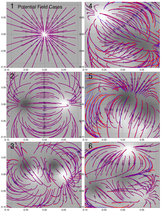
Figure 3.: Test cases # 1-6 are shown, consisting of a unipolar (#1: top left), a dipolar (#2: middle left), a quadrupolar (#3: bottom left), and three decapolar cases (#4-6: panels on right side). The displays contain the line-of-sight magnetograms (greyscale), the theoretically simulated loop field lines (red curves), and the overlaid best-fit NLFFF field lines (blue curves). The starting point of the calculated field lines are indicated with diamonds (at midpoint of loops, $q_{\rm loop}=0.5$). Note the small amount of misalignment, ranging from $\mu=0.0^{\circ}$ (# 1) to $\mu=6.6^{\circ}$ (#5) (the values are given in Table 2).

Table 2.: Best-fit parameters of forward-fitting of the NLFFF model to potential field cases (with $\alpha_{j}=0$), using standard settings of the forward-fitting code (Table 1). The columns contain the case #=1-6, the number of magnetic charges $N_{\rm mag}$, the number of loop field lines $N_{\rm loop}$, the mean misalignment angle $\mu$, the mean best-fit force-free parameter $\alpha$ per loop, the divergence-freeness figure of merit $L_{\rm d}$, the force-freeness figure of merit $L_{\rm f}$, and the computation time $t_{\rm CPU}$ of the forward-fitting module 6. The last lines of the Table contain the means and standard deviations $\sigma$ of the six cases.

#	$N_{\rm mag}$	$N_{\rm loop}$	$\mu$	$\alpha$	$L_{\rm d}$	$L_{\rm f}$	$t_{\rm CPU}$
1	1	61	$0.0^{\circ}$	$0.00$	0.000001	0.000001	2 s
2	2	91	$2.7^{\circ}$	$0.00$	0.000002	0.000002	9 s
3	4	91	$3.8^{\circ}$	$-0.03$	0.000007	0.000008	23 s
4	10	107	$3.0^{\circ}$	$-0.06$	0.000001	0.000008	111 s
5	10	95	$6.6^{\circ}$	$-0.08$	0.000017	0.000480	117 s
6	10	98	$4.2^{\circ}$	$-0.39$	0.000003	0.000003	105 s
Mean			$3.4^{\circ}$	$-0.09$	0.000005	0.000084	61 s
$\pm\sigma$			$\pm 2.1^{\circ}$	$\pm 0.15$	$\pm 0.000006$	$\pm$0.000194	$\pm 55$ s

3 Potential Field Tests

A first set of six test cases consists of potential field models (with $\alpha_{j}=0$), including a unipolar charge, a dipole, a quadrupole, and three cases with 10 randomly distributed magnetic sources, identical to Cases #1-3 in Paper I, and to Cases #7-9 (but with $\alpha_{j}$ set to zero). For each of these six cases we show in Figure 3 a set of field lines calculated from the model (Figure 3, red curves), and a set of field lines obtained from forward-fitting with our NLFFF code. The agreement between the two sets of field lines can be expressed by the mean 3D misalignment angle $\mu$ (Equation (2)), which is found to be very small, within a range of $\mu=0.0^{\circ}-6.6^{\circ}$, or $\mu=3.4^{\circ}\pm 2.1^{\circ}$. The individual values are listed in Table 2 (forth column). While this mostly represents a test of the accuracy of module 5 (forward-fitting of potential-field parameters), the algorithm treats the force-free parameter $\alpha_{j}$ as a variable too, and thus it represents also a test of the accuracy in determining this parameter in general. Compared with the theoretical value as it was set in the simulation of the input magnetogram ($\alpha_{j}=0$), the best-fit values are found to be $\alpha=-0.09\pm 0.15$ (Table 2, fifth column), which corresponds to $\Delta N_{\rm twist}=bl/2\pi=\alpha l/4\pi=\pm 0.0018$ twist turns over the length $l=0.05\pi=0.157$ solar radii of a typical field line (see definitions in Equations (16)–(17) in Paper I). Thus the uncertainty of our forward-fitting corresponds to less than $\pm 0.2$% of a full twist turn over a loop length. Another measure of the quality of the NLFFF forward-fit is the divergence-freeness, which is found to be $L_{\rm d}=(5\pm 6)\times 10^{-6}$ (Table 2, sixth column), and the force-freeness, which is found to be $L_{\rm f}=(84\pm 194)\times 10^{-6}$ (Table 2, seventh column), both being extremely accurate. The average computation time for the NLFFF forward-fitting runs of potential field cases was found to be $t_{\rm CPU}\approx 61$ s (on a Mac OS X with $2\times 3.2$ GHz Quad-Core Intel Xeon processor and 32 GB 800 MHz DDR2 FB-DIMM Memory).

Table 3.: Best-fit parameters of forward-fitting of the NLFFF model to potential field cases (with $\alpha_{j}=0$), using some non-standard settings in the spatial resolution $\Delta s/\Delta x$ of calculated field lines, the number of magnetic source compoonents $N_{\rm mag}$, the starting point of field line extrapolation $q_{\rm loop}$, the relative weighting of loop and vector magnetograph data $q_{\rm v}$, but otherwise standard settings as listed in Table 1.

$\Delta s$	$N_{\rm mag}$	$q_{\rm loop}$	$q_{\rm v}$	$\mu$	$\alpha$	$L_{\rm d}[10^{-6}]$	$t_{\rm CPU}$
$\times 1.0$	$\times 1$	1.0	0.0	$3.4^{\circ}\pm 2.1^{\circ}$	$-0.09\pm 0.15$	$5\pm 6$	$61\pm 55$ s
$\times 0.5$	$\times 1$	1.0	0.0	$3.4^{\circ}\pm 2.1^{\circ}$	$-0.08\pm 0.14$	$5\pm 6$	$70\pm 66$ s
$\times 1.0$	$\times 2$	1.0	0.0	$3.2^{\circ}\pm 1.7^{\circ}$	$0.03\pm 0.13$	$10\pm 19$	$228\pm 233$ s
$\times 1.0$	$\times 1$	0.0	0.0	$3.4^{\circ}\pm 2.1^{\circ}$	$-0.07\pm 0.16$	$5\pm 6$	$71\pm 66$ s
$\times 1.0$	$\times 1$	1.0	1.0	$1.8^{\circ}\pm 2.3^{\circ}$	$-0.07\pm 0.10$	$3\pm 3$	$314\pm 290$ s

We performed also some parametric studies to explore the accuracy of the forward-fitting code as a function of some control parameters that are different from the standard settings given in Table 1. We list the results in Table 3. If we increase the spatial resolution of the field line extrapolation to $\Delta s/\Delta x=0.5$, the accuracy of the field lines does not change, neither in terms of the the mean misalignment angle nor in the divergence-freeness figure of merit (Table 3, second line). Increasing the number of magnetic components in the decomposition of magnetograms does not improve the accuracy for the potential-field cases (e.g., by a factor of two compared with the simulated numbers of $N_{\rm mag}=1,2,4,10$), but degrades the divergence-freeness and force-freeness and increases the computation time by a factor of $\approx 4$ (Table 3, third line). Starting the field line extrapolation at the footpoints ($q_{\rm loop}=0.0$), rather than from the loop midpoints ($q_{\rm loop}=0.5$), leads to no significant improvement (Table 3, fourth line). Changing the weighting of coronal loop constraints ($q_{\rm v}=0$) to using only photospheric vector magnetograph data ($q_{\rm v}=1$) improves the misalignment to $\mu=1.8^{\circ}\pm 2.3^{\circ}$, which represents an improvement in the accuracy by about a factor of two, but requires about five times more computation time. Thus, the accuracy in fitting potential field cases is fairly robust and does not depend the detailed setting of control parameters, except for the weigthing of photospheric versus coronal constraints.

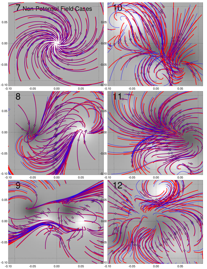
Figure 4.: Test cases # 7-12 are shown, consisting of a unipolar (#7: top left), a dipolar (#8: middle left), a quadrupolar (#9: bottom left), and three decapolar cases (#10-12: panels on right side). The displays contain the line-of-sight magnetograms (greyscale), the theoretically simulated loop field lines (red curves), and the overlaid best-fit NLFFF field lines (blue curves). The starting points of the calculated field lines are indicated with diamonds (at midpoint of loops, $q_{\rm loop}=0.5$). The misalignment angles between the theoretical models and the best fits are listed in Table 4. Note the huge difference of field line topologies compared with the potential-field cases (shown in Figure 3), although the line-of-sight magnetograms are identical.

4 Forward-Fitting to Quasi-NLFFF Models

Now we present the first tests of forward-fitting to non-potential fields (with $\alpha_{j}\neq 0$), numbered as test cases # 7-12. These six cases have the same line-of-sight magnetograms $B_{z}(x,y)$ or magnetic charges $(B_{j},x_{j},y_{j},z_{j})$ as the potential-field cases # 1-6, but have a different twist or force-free parameter $\alpha_{j}$. We show the magnetograms and the theoretical field lines of the models in Figure 4 (red curves), and the best-fit field lines of our NLFFF forward-fitting code in Figure 4 (blue curves), using standard control parameter settings (Table 1). The misalignment between these two sets of simulated and forward-fitted field lines amounts to $\mu=0.7^{\circ}-12.8^{\circ}$, or $\mu=5.1^{\circ}\pm 4.3^{\circ}$ (Table 4, fourth column). These test results are quite satisfactory, first of all since the difference between the theoretical and best-fit field lines in Figure 4 are hardly recognizable by eye, and thus will suffice for all practical purposes, and secondly, the misalignment is about an order of magnitude smaller than found between traditional NLFFF codes and stereoscopically triangulated coronal loops ($\mu\approx 24^{\circ}-44^{\circ}$; DeRosa et al., 2009). We see that the force-free parameters vary substantially, in a range of $\alpha=6\pm 40$ (solar radius^-1) (Table 4, 5th column), which translates into a number $N_{\rm twist}=\alpha l/4\pi\approx 0.5$ of (full) twist turns over a typical loop length. The merit of figure for the divergence-freeness is $L_{\rm d}=(0.8\pm 0.5)\times 10^{-3}$ (Table 4, sixth column), and the merit of figure for the force-freeness is $L_{\rm f}=(2.3\pm 2.3)\times 10^{-3}$ (Table 4, seventh column). The computation time is ($t_{\rm CPU}\approx 100$ s) less than a factor of two longer than for the potential-field cases (Table 2).

Table 4.: Best-fit parameters of forward-fitting of the NLFFF model to non-potential field cases (with $\alpha_{j}\neq 0$), using standard settings of the forward-fitting code (Table 1). The columns contain the cases #=7-12, the number of magnetic charges $N_{\rm mag}$, the number of loop field lines $N_{\rm loop}$, the mean misalignment angle $\mu$, the mean input force-free $\alpha$ parameter values, the divergence-freeness figure of merit $L_{\rm d}$, the force-freeness figure of merit $L_{\rm f}$, and the computation time $t_{\rm CPU}$ of the forward-fitting module 6.

#	$N_{\rm mag}$	$N_{\rm loop}$	$\mu$	$\alpha$	$L_{\rm d}$	$L_{\rm f}$	$t_{\rm CPU}$
7	1	66	$0.7^{\circ}$	$-20$	0.000453	0.000299	2 s
8	2	85	$2.2^{\circ}$	$-20\pm 1$	0.000253	0.000104	8 s
9	4	82	$3.6^{\circ}$	$-30\pm 12$	0.000727	0.000691	21 s
10	10	89	$12.8^{\circ}$	$29\pm 40$	0.001813	0.004672	118 s
11	10	89	$4.5^{\circ}$	$2\pm 102$	0.000784	0.003123	179 s
12	10	99	$7.1^{\circ}$	$74\pm 62$	0.000976	0.005334	271 s
Mean			$5.1^{\circ}$	6	0.000834	0.002370	99 s
$\pm\sigma$			$\pm 4.3^{\circ}$	$\pm 40$	$\pm 0.000543$	$\pm$0.002319	$\pm 109$ s

In order to achieve the most accurate performance of our code we explored also other control parameter settings than the standard parameters given in Table 1. Instead of using the hierarchical $\alpha$-zone subdivision as shown in Figure 2 (Meth=A), we tested also other methods, such as subdivision by magnetically conjugate pairs of magnetic charges (Meth=B), or subdivision by magnetically conjugate loop footpoints (Meth=C). In 90% of the test cases all three methods converged to the same minimum misalignment angle within $\pm 0.1^{\circ}$, but for the 10% of discrepant cases method $A$ performed always best, so we conclude that method $A$ is the most robust one.

Increasing the resolution of calculating field lines to $\Delta s=0.5\Delta x$ does not improve the misalignment ($\mu=5.1^{\circ}\pm 4.3^{\circ}$; Table 5, second case); Increasing the number of magnetic sources by a factor of two does not improve the misalignment significantly either (Table 5; third case). Starting the field line extrapolation at the footpoints ($q_{\rm loop}=0.0$) rather than from the loop midpoints, has no effect either (Table 5; forth case). However, the change of replacing the coronal ($q_{\rm v}=0$) to photospheric constraints, using 3D vector magnetograph data $q_{\rm v}=1$ does improve the best fits substantially, but is more costly in computation time (Table 5, fifth case). The reason for this improvement is probably that photoshperic field vectors are more uniformly distributed than coronal loops, but coronal constraints are more important when the photospheric magnetic field is not force-free.

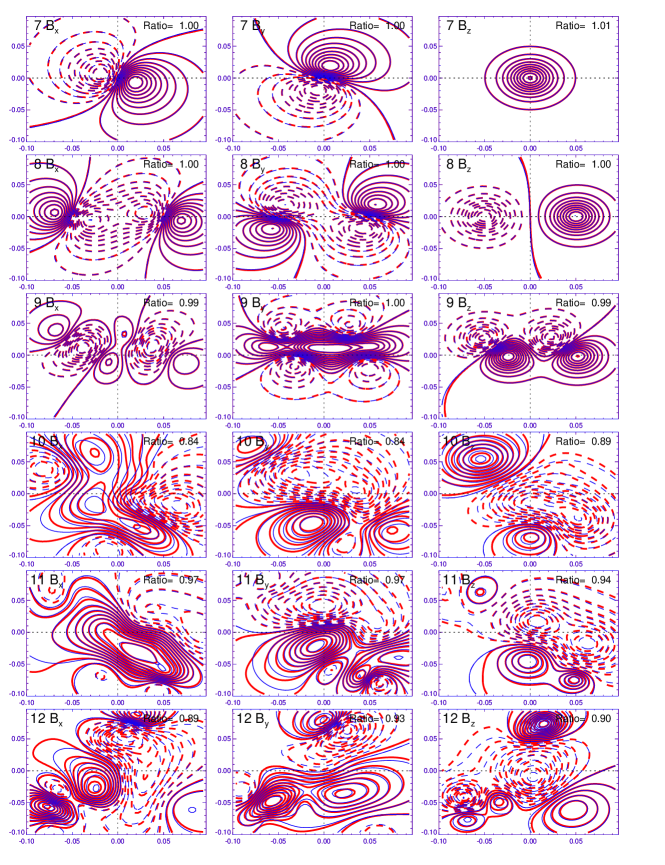
Figure 5.: Contour maps of magnetic field component maps $B_{x}(x,y)$ (left column), $B_{y}(x,y)$ (middle column), and line-of-sight component $B_{z}(x,y)$ at the photospheric level for cases #7-12 (rows), shown with red contours (solid for positive and dashed for negative magnetic polarity). The best fits that result from the decomposition of the line-of-sight component are shown with blue curves, and the mean ratio of the absolute magnetic field strengths between the best fit and the model are indicated in each frame.

Figure 6.: Contour maps of the force-free parameter $|\alpha(x,y)|$ of the simulated models (top and third row) and best-fit solutions (second and forth row), for the six cases # 7-12.

Table 5.: Best-fit parameters of forward-fitting of the NLFFF model to potential field cases (with $\alpha_{j}=0$), using some non-standard settings in the spatial resolution $\Delta s/\Delta x$ of calculated field lines, the number of magnetic source compoonents $N_{\rm mag}$, the starting point of field line extrapolation $q_{\rm loop}$, the relative weighting of loop and vector magnetograph data $q_{\rm v}$, but otherwise standard settings as listed in Table 1.

$\Delta s$	$N_{\rm mag}$	$q_{\rm loop}$	$q_{\rm v}$	$\mu$	$L_{\rm d}[10^{-3}]$	$L_{\rm f}[10^{-3}]$	$t_{\rm CPU}$
$\times 1.0$	$\times 1$	1.0	0.0	$5.1^{\circ}\pm 4.3^{\circ}$	$0.8\pm 0.5$	$2.3\pm 2.3$	$99\pm 109$ s
$\times 0.5$	$\times 1$	1.0	0.0	$5.1^{\circ}\pm 4.3^{\circ}$	$0.8\pm 0.6$	$2.3\pm 2.3$	$100\pm 110$ s
$\times 1.0$	$\times 2$	1.0	0.0	$4.5^{\circ}\pm 2.9^{\circ}$	$0.7\pm 0.3$	$2.1\pm 2.1$	$303\pm 307$ s
$\times 1.0$	$\times 1$	0.0	0.0	$5.1^{\circ}\pm 4.3^{\circ}$	$0.8\pm 0.5$	$2.4\pm 2.3$	$100\pm 110$ s
$\times 1.0$	$\times 1$	1.0	1.0	$3.4^{\circ}\pm 3.6^{\circ}$	$0.7\pm 0.3$	$2.2\pm 2.1$	$459\pm 342$ s

The agreement between the best forward-fitting solutions of the magnetic field components $(B_{x},B_{y},B_{z})$ and the model are shown in Figure 5. Note that only the line-of-sight magnetogram $B_{z}(x,y,z_{\rm ph})$ was used as input to the forward-fitting code, for standard control parameter settings ($q_{\rm v}=0$). For these tests, the code predicts the transverse component maps $B_{x}(x,y)$ and $B_{y}(x,y)$, which is quite satisfactory for this set of tests, as Figure 5 demonstrates. The mean ratios of the absolute magnetic field strenghts are accurate within a few percents (indicated in each panel of Figure 5).

Figure 7.: Scatter plot of the best-fit force-free parameters $\alpha_{\rm fit}(x,y,z_{\rm ph})$ of every map pixel $(x,y)$ versus the corresponding value $\alpha_{\rm sim}(x,y,z_{\rm ph})$ of the simulated models for the six cases # 7-12. The mean and standard deviation of the ratio $\alpha_{\rm fit}/\alpha_{\rm sim}$ is indicated in each panel.

Figure 8.: Scatter plot of the best-fit force-free parameters $\alpha_{\rm fit}$ averaged from each fitted coronal loop versus the corresponding value $\alpha_{\rm sim}$ of the simulated model loops for the six cases # 7-12. The vertical error bars indicate the standard deviation of the spatial variation of $\alpha_{\rm fit}(s)$ along each loop. The mean and standard deviation of the ratio $\alpha_{\rm fit}/\alpha_{\rm sim}$ is indicated in each panel.

The force-free parameter $\alpha$ is shown as a photospheric map $|\alpha(x,y,z_{\rm ph})|$ for the model (Figure 6, top and third row) and for the forward-fitting solution (Figure 6, second and forth row). The comparison can be quantified by the ratio of the two values, which agrees within a few percents. A sensible test is also to display a scatterplot of the best-fit $\alpha$-values versus the model $\alpha$-values for each pixel of a photospheric map (Figure 7), or averaged along each of the fitted coronal loops (Figure 8). The ratios of the two quantities ranges from $\alpha_{\rm fit}/\alpha_{\rm loop}=0.99\pm 0.00$ for the best case (#7, Figure 8 top left) to $\alpha_{\rm fit}/\alpha_{\rm loop}=0.88\pm 0.29$ for the worst case (#12, Figure 6 bottom right). Our forward-fitting code retrieves the correct sign of the $\alpha$-parameter in all cases, and their absolute values agree within a few percents with the theoretical model. Thus we conclude that the convergence behavior of our forward-fitting code is quite satisfactory, because it retrieves the force-free $\alpha$-parameters with high accuracy, at least for the given parameterization.

5 Forward-Fitting to Low and Lou (1990) Model

The foregoing tests were necessary to verify how accurately the forward-fitting code can retrieve the solution with many free parameters (from $n_{\rm free}=5,...,50$), which represents a numerical convergence test. Of course, because the same parameterization is used in simulating the input data as in the model that is forward-fitted to the simulated data, this represents the most favorable condition where the model parameterization is adequate for the input data. Moreover, the simulated data were only force-free to second order, so we cannot use the force-freeness figure of merit calculated from the solution as an absolute criterion to evaluate how accurate the forward-fitting solution fulfills Maxwell’s equations. So, the foregoing tests do not tell us whether the model parameterization of the forward-fitting code is adequate for arbitrary data, and how physical the solution is.

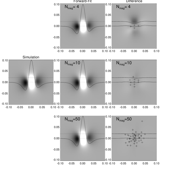
Figure 9.: The decomposition of line-of-sight magnetogram $B_{z}(x,y)$ (simulation in left middle frame) of the Low and Lou (1990) model is shown for three trials with different numbers of magnetic components ($N_{\rm mag}=4,10,50$, first, second, and thrid row). The locations of the center positions of the magnetic components is shown with crosses in the difference images (right-hand panels). Two profiles across the middle of the magnetogram are also shown (solid curves).

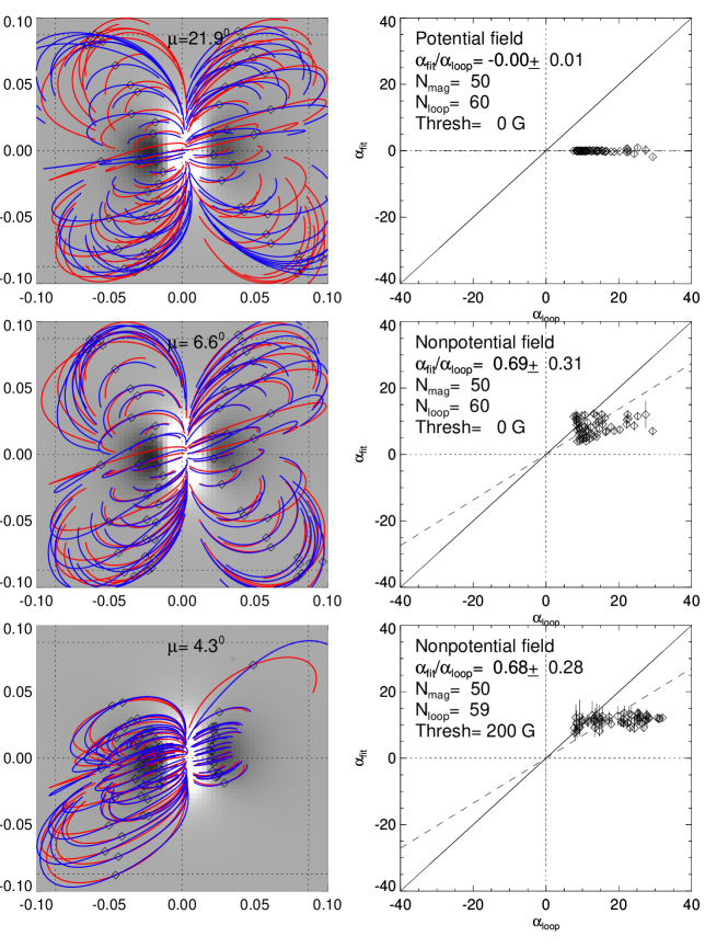
Figure 10.: Potential field calculation (top) and forward-fitting of a nonpotential (quasi-NLFFF) model (middle and bottom) to different sets (Thresh=0, 200 G) of $N_{\rm loop}\approx 60$ coronal loops, which represent an accurate nonlinear force-free field solution of the Low and Lou (1991) model. The model loops are outlined in red color, and the best-fit field lines in blue color. The average misalignment angle $\mu$ is indicated in each panel. The photospheric magnetogram is rendered with a greyscale. A scatterplot of the best-fit $\alpha_{\rm fit}$-parameters averaged along each loop versus the model parameters $\alpha_{\rm model}$ are shown in the right-hand panels.

We conduct now a test that generates the input data with a completely different parameterization than our model and fit a non-potential field case that is exactly force-free, which is provided by analytical NLFFF solutions of the Low and Lou (1990) model, described and used also in Malanushenko et al.(2009). The particular solution we are using is defined by the parameters $(a=0.6,n=2.0)$, where $a$ is a Grad-Shafranov constant and $n$ is the harmonic number of the Legendre polynomial.

The line-of-sight magnetogram $B_{z}(x,y)$ of the Low and Lou case consists of three smooth patches with an elliptical geometry, where the central patch has a positive magnetic polarity, and the eastern and western patch a negative polarity (see greyscale image in Figure 9 in left panel). The ideal number of decomposed features in the magnetogram is not known a priori, because a too small number leaves too large residuals of magnetic flux that is not accounted for in the forward-fit, while a too large number leads to overlapping magnetic field components and force-free $\alpha$-parameter zones, which may jeopardize the quality of forward-fitting (which works best for spatially non-overlapping and independent zones). We show three different trials with $N_{\rm mag}=4,10,50$ in Figure 9. The forward-fitted magnetograms and the difference images with respect to the input magnetogram are also shown in Figure 9. The residuals in the difference images have a mean and standard deviation of $(B_{\rm fit}-B_{\rm model})/B_{\rm max}=0.0022\pm 0.0243$ for $N_{\rm mag}=4$; $-0.0005\pm 0.0082$ for $N_{\rm mag}=10$; and $-0.0016\pm 0.0043$ for $N_{\rm mag}=50$, respectively. Thus, the forward-fitted magnetograms agree with the Low and Low (1990) model within $\lower 1.72218pt\hbox{$\;\buildrel<\over{\scriptstyle\sim}\;$}1\%$ of the magnetic flux. Note that the parameters that decompose the line-of-sight magnetogram make up 80% of the free parameters in our forward-fitting model, fully determine the potential field extrapolation, but ignore the force-free $\alpha$-parameters so far. The potential field solution for the Low and Lou (1990) model is shown in Figure 10 (top panel), for a decomposition of $N_{\rm mag}=50$ magnetic components, for a set of $N_{\rm loop}=60$ loops. The resulting mean misalignment between the model and the potential field is $\mu=21.9^{\circ}$ (Table 6, first line), and $\mu=30.8^{\circ}$ for $N_{\rm mag}=10$, respectively.

Table 6.: Best-fit results of forward-fitting to the Low and Lou (1990) model, using the following parameter settings: the number of magnetic source compoonents $N_{\rm mag}=10,50$, the threshold of the magnetic field for selected loops Thresh=0, 200 G, but otherwise standard settings as listed in Table 1. The results are quantified by the number of fitted loops $n_{\rm loop}$, the mean misalignment angle $\mu$ (degrees), the ratio of the fitted to the model input force-free parameter, $\alpha_{\rm fit}/\alpha_{\rm model}$, the divergence-freeness $L_{\rm d}$, the force-freeness $L_{\rm f}$, and the computation time $t_{\rm CPU}$ (s).

$N_{\rm mag}$	Thresh	$n_{\rm loop}$	$\mu$	$\alpha_{\rm fit}/\alpha_{\rm model}$	$L_{\rm d}$	$L_{\rm f}$	$t_{\rm CPU}$
	[G]		(deg)				(s)
50	0	60	21.9∘	$0.00\pm 0.02$	0.000021	0.000023	0
10	0	60	12.7∘	$0.66\pm 0.43$	0.000083	0.000751	257
50	0	60	6.6∘	$0.69\pm 0.31$	0.000045	0.000082	1359
10	200	59	6.1∘	$0.63\pm 0.22$	0.000121	0.000617	123
50	200	59	4.3∘	$0.68\pm 0.28$	0.000084	0.000174	1338

We forward-fitted several hundred runs to the Low and Lou (1990) model with different parameter settings (Table 1) and list the results of a selection of four cases in Table 6, and two cases thereof in Figure 10. For $N_{\rm mag}=50$ and a threshold of Thresh=0 G we find a solution that has only a misalignment of $\mu=6.6^{\circ}$ (Figure 10, middle panel, and Table 6, third line). This case retrieves the force-free parameter $\alpha$ with an average ratio of $\alpha_{\rm fit}/\alpha_{\rm model}=0.69\pm 0.31$ (Figure 10, middle right panel) for the 60 loops shown. The divergence-freeness and force-freeness amount to $L_{\rm d}=4.5\times 10^{-5}$ and $L_{\rm f}=8.2\times 10^{-5}$. If we select a set of coronal loops with only strong magnetic field strengths at the footpoints (Thres=200 G), the misalignment improves to $\mu=4.3^{\circ}$ (Figure 10, bottom left panel), while the accuracy of the retrieved $\alpha$-values remains about the same ($\alpha_{\rm fit}/\alpha_{\rm model}=0.68\pm 0.28$ (Figure 10, bottom right panel). It appears that our forward-fitting code always underestimates the values in loops with the highest $\alpha$-parameter, which was not the case in all of our previous simulations (Figure 8). It appears that the elliptical shape of magnetic patches could be responsible for this underestimate, while it did not occur for spherical shapes of magnetic patches (Simulation runs #7-12) described in Section 4. Nevertheless, the achieved small amount of misalignment down to $\mu=4.3^{\circ}$ yields a good approximation to a nonlinear force-free field that is sufficiently accurate for most practical purposes of coronal field modeling and can be obtained in a relatively short computation time. The computation times for the five runs listed in Table 6 amounted to $t_{\rm CPU}\approx 2-20$ minutes. We obtained even higher accuracies down to misalingmens of $\mu\lower 1.72218pt\hbox{$\;\buildrel<\over{\scriptstyle\sim}\;$}1^{\circ}$ for smaller subgroups of coronal loops that were localized in partial domains of the active region.

6 Discussion and Conclusions

In this study we developed a numeric code that accomplishes (second-order) nonlinear force-free field fast forward-fitting of combined photospheric magnetogram and coronal loop data. The goal of this code is to compute a realistic magnetic field of a solar active region. Previously developed magnetic field extrapolation codes used either photospheric data only, such as potential-field source surface (PFSS) codes (e.g., Altschuler and Newkirk, 1969) and nonlinear force-free field (NLFFF) codes (e.g., Yang et al., 1986; Wheatland et al., 2000, 2006; Wiegelmann, 2004; Schrijver et al., 2005, 2006; Amari et al., 2006; Valori et al., 2007; Metcalf et al., 2008; DeRosa et al., 2009; Malanushenko et al., 2009), or (stereoscopically triangulated) coronal loop data only (Sandman et al., 2009; Sandman and Aschwanden, 2011). There are only very few attempts where both photospheric and coronal data constraints were used together to obtain a magnetic field solution, using either a potential field model with unipolar buried charges that could be forward-fitted to the observed loops (Aschwanden and Sandman, 2011), a linear force-free field (Feng et al., 2007a,b), or a NLFFF code (Malanushenko et al., 2009, 2011). For special geometries, potential field stretching methods (Gary and Alexander, 1999) or a minimum dissipative rate method for non-forcefree fields have also been explored (Gary, 2009).

The new approach of including coronal magnetic field data, in form of stereoscopically triangulated loop 3D coordinates, requires a true forward-fitting approach, while the traditional use of photospheric magnetogram (or vector magnetograph) data represents an extrapolation method from given boundary constraints. Both methods require numerous iterations, and thus are computing-intensive, but the classical forward-fitting method requires a suitable parameterization of a magnetic field model, while extrapolation methods put no constraints on the functional form of the solutions (such as the 3D geometry of magnetic field lines). Thus, the new approach developed here makes use of a parameterization of the 3D magnetic field model in terms of analytical functions that can be fitted relatively fast to the given coronal constraints, but may lack the absolute generality of nonlinear force-free field solutions that NLFFF codes are providing. However, our analytical NLFFF model, which is accurate to second-order (Paper I), probably represents one of the most general parameterizations that is possible with a minimum of free parameters, adapted to uniformly twisted field lines. The parameter space given by this model represents a particular class of quasi-forcefree solutions, which is supposed to be most suitable for a superposition of twisted field line structures, but only fitting to real data can reveal how useful and suitable our model is for applications to solar data.

In this study we described the numeric code, which is based on the analytical second-order solutions derived in Paper I, and performed test with 12 simulated cases (six potential and six non-potential), as well as with an analytical NLFFF solution of the Low and Lou (1990) model. The forward-fitting to the 12 simulated cases demonstrated (i) the satisfactory convergence behavior of the forward-fitting code (with mean misalignment angles of $\mu=3.4^{\circ}\pm 2.1^{\circ}$ for potential field cases (see Table 2), and $\mu=5.1^{\circ}\pm 4.3^{\circ}$ for non-potential field cases (see Table 4), (ii) the relatively fast computation speed (from $\lower 1.72218pt\hbox{$\;\buildrel<\over{\scriptstyle\sim}\;$}1$ s to $\lower 1.72218pt\hbox{$\;\buildrel<\over{\scriptstyle\sim}\;$}10$ min); and (iii) the high fidelity of retrieved force-free $\alpha$-parameters ($\alpha_{\rm fit}/\alpha_{\rm model}\approx 0.9-1.0$; see Figure 8). The additional test of forward-fitting to the analytical solution of Low and Lou (1990) data yielded similar results, i.e., satisfactory convergence behavior (with mean misalignment angles of $\mu=4.3^{\circ}-6.6^{\circ}$ for two subsets of loops, see Figure 10), (ii) relatively fast computation speed ($t_{\rm CPU}\approx 2-20$ min); and (iii) the fidelity of retrieved force-free $\alpha$-parameters ($\alpha_{\rm fit}/\alpha_{\rm model}\approx 0.7\pm 0.3$; see Figure 10). The only significant difference of the second test is the trend of underestimating the $\alpha$-parameter for those loops with the highest $\alpha$-values, by a factor of $\lower 1.72218pt\hbox{$\;\buildrel>\over{\scriptstyle\sim}\;$}0.5$. However, if the loops with the highest $\alpha$-values are fitted individually, the code retrieves the correct $\alpha$-value. It is not clear whether this feature of the code is related to the geomerical shape of the magnetic concentrations in the magnetogram, which is spherical in our simulation and forward-fitting model, but elliptical in the Low and Lou (1990) case. We simulated the elliptical magnetic sources of the Low and Lou (1990) model by a superposition of spherical sources and found that the code retrieves the correct $\alpha$-values for each loop (within a few percent accuracy). It is possible that the geometric shape of the Low and Lou (1990) model, which represents a special class of nonlinear force-free solutions anyway (in terms of Legendre polynomials) cannot efficiently be parameterized with a small number of spherical components, which is the intrinsic parameterization of our code. Anyway, since the Low and Lou (1990) model represents also a very special subclass of nonlinear force-free solutions that may or may not be adequate to model real solar active regions, it may not matter much for the performance of our code with real solar data.

After having tested our numeric code we can proceed to apply it to solar data, such as active regions observed with STEREO since 2007, for which stereoscopic triangulation of coronal loops is available (Feng et al., 2007a,b; Aschwanden and Sandman, 2010; Aschwanden et al., 2012a,b). The second-order NLFFF approximations of our code may be used as an initial guess for other more accurate NLFFF codes, resulting into a significantly shorter computation time. Other future developments may involve the reduction of coronal constraints from 3D to 2D coordiantes, which can be furnished by automatic loop tracing codes (e.g., Aschwanden et al., 2008; Aschwanden, 2010; and references therein) and does not require the availability of STEREO data. However, non-STEREO data provide less rigorous constraints for coronal loop modeling, and thus increase the ambiguity of force-free field solutions. Nevertheless, more realistic coronal magnetic field models seem now in the grasp of our computation methods, which has countless benefits for many research problems in solar physics.

Part of the work was supported by NASA contract NNG 04EA00C of the SDO/AIA instrument and the NASA STEREO mission under NRL contract N00173-02-C-2035.

References

Altschuler, M.D., Newkirk, G.Jr.: 1969, Solar Phys. 9, 131.

Amari, T., Boulmezaoud, T.Z., Aly, J.J.: 2006, Astron. Astrophys. 446, 691.

Aschwanden, M.J.: 2004, Physics of the Solar Corona. An Introduction, Praxis Publishing Co., Chichester UK, and Springer, Berlin, Section 5.3.

Aschwanden, M.J., Lee, J.K., Gary, G.A., Smith, M., Inhester, B.: 2008, Solar Phys. 248, 359.

Aschwanden, M.J.: 2010, Solar Phys. 262, 399.

Aschwanden, M.J., Sandman, A.W.: 2010, Astronom. J. 140, 723.

Aschwanden, M.J.: 2012, Solar Phys. this volume; Paper I.

Aschwanden, M.J., Wülser, J.P., Nitta, N.V., Lemen, J.R., DeRosa, M., Malanushenko, A.: 2012a, Astrophys. J. submitted.

Aschwanden, M.J., Wülser, J.P., Nitta, N.V., Lemen, J.R.: 2012b, Solar Phys. in press.

DeRosa, M.L., Schrijver, C.J., Barnes, G., Leka, K.D., Lites, B.W., Aschwanden, M.J., et al.: 2009, Astrophys. J. 696, 1780.

Feng, L., Inhester, B., Solanki, S., Wiegelmann, T., Podlipnik, B., Howard, R.A., Wülser, J.P.: 2007a, Astrophys. J. Lett. 671, L205.

Feng, L., Wiegelmann, T., Inhester, B., Solanki, S., Gan, W.Q., Ruan, P.: 2007b, Solar Phys. 241, 235.

Gary, A., Alexander, D.: 1999, Solar Phys. 186, 123.

Gary, G.A.: 2009, Solar Phys. 257, 271.

Grad, H., Rubin, H.: 1958, Proc. 2nd UN Int. Conf. Peaceful Uses of Atomic Energy, 31, 190.

Low, B.C., Lou, Y.Q.: 1990, Astrophys. J. 352, 343.

Malanushenko, A., Longcope, D.W., McKenzie, D.E.: 2009, Astrophys. J. 707, 1044.

Malanushenko, A., Yusuf, M.H., Longcope, D.W.: 2011, Astrophys. J. 736, 97.

Metcalf, T.R., Jiao, L., Uitenbroek, H., McClymont, A.N., Canfield,R.C.: 1995, Astrophys. J. 439, 474.

Metcalf, T.R., DeRosa, M.L., Schrijver, C.J., Barnes, G., van Ballegooijen, A.A., Wiegelmann, T., Wheatland, M.S., Valori, G., McTiernan, J.M.: 2008, Solar Phys. 247, 269.

Press, W.H., Flannery, B.P., Teukolsky, S.A., Vetterling, W.T.: 1986, Numerical Recipes, The Art of Scientific Computing, Cambridge University Press, Cambridge, 294.

Ruan, P., Wiegelmann, T., Inhester, B., Neukirch, T., Solanki, S.K., Feng, L.: 2008, Astron. Astrophys. 481, 827.

Sandman, A., Aschwanden, M.J., DeRosa, M., Wülser, J.P., Alexander, D.: 2009, Solar Phys. 259, 1.

Sandman, A.W., Aschwanden, M.J.: 2011, Solar Phys. 270, 503.

Schrijver, C.J., DeRosa, M.L., Metcalf, T.R., Liu, Y., McTiernan, J., Regnier, S., Valori, G., Wheatland, M.S., Wiegelmann, T.: 2006, Solar Phys. 235, 161.

Schrijver, C.J., DeRosa, M.L., Metcalf, T., Barnes, G., Lites, B., Tarbell, T., et al.: 2008, Astrophys. J. 675, 1637.

Valori, G., Kliem, B., Fuhrmann, M.: 2007, Solar Phys. 245, 263.

Wheatland, M.S., Sturrock, P.A., Roumeliotis, G.: 2000, Astrophys. J. 540, 1150.

Wheatland, M.S.: 2006, Solar Phys. 238, 29.

Wiegelmann, T., Neukirch, T.: 2002, Solar Phys. 208, 233.

Wiegelmann, T., Inhester, B.: 2003, Solar Phys. 214, 287.

Wiegelmann, T.: 2004, Solar Phys. 219, 87.

Wiegelmann, T., Lagg, A., Solanki, S.K., Inhester, B., Woch, J.: 2005 Astron. Astrophys. 433, 701.

Wiegelmann, T., Inhester, B.: 2006, Solar Phys. 236, 25.

Yang, W.H., Sturrock, P.A., Antiochos, S.K.: 1986, Astrophys. J. 309, 383.