A Nonlinear Force-Free Magnetic Field Approximation Suitable for Fast Forward-Fitting to Coronal Loops. I. Theory

Abstract

We derive an analytical approximation of nonlinear force-free magnetic field solutions (NLFFF) that can efficiently be used for fast forward-fitting to solar magnetic data, constrained either by observed line-of-sight magnetograms and stereoscopically triangulated coronal loops, or by 3D vector-magnetograph data. The derived NLFFF solutions provide the magnetic field components $B_{x}({\bf x})$, $B_{y}({\bf x})$, $B_{z}({\bf x})$, the force-free parameter $\alpha({\bf x})$, the electric current density ${\bf j}({\bf x})$, and are accurate to second-order (of the nonlinear force-free $\alpha$-parameter). The explicit expressions of a force-free field can easily be applied to modeling or forward-fitting of many coronal phenomena.

1 Introduction

The coronal magnetic field can be constrained in a number of ways, such as by extrapolation of photospheric magnetograms or vector-magnetograph data, by radio observations of gyroresonance layers above sunspots, of by coronal seismology of oscillating loops. Before the advent of the STEREO mission, attempts were made to model observed coronal loops with stretched potential field solutions (Gary and Alexander, 1999), to fit a linear force-free model with solar-rotation stereoscopy (Wiegelmann and Neukirch, 2002; Feng et al., 2007a), by tomographic reconstruction with magnetohydrostatic constraints (Wiegelmann and Inhester, 2003; Ruan et al., 2008), by magnetic modeling applied to spectropolarimetric loop detections (Wiegelmann et al., 2005), or by magnetic field supported stereoscopic loop triangulation (Wiegelmann and Inhester, 2006; Conlon and Gallagher, 2010). Recently, stereoscopic triangulation of coronal loops with the STEREO mission became available, which constrains the 3D geometry of coronal magnetic field lines (Aschwanden et al., 2008; Aschwanden, 2009). The plethora of coronal high-resolution data allows us now to compare different magnetic models and to test whether they are self-consistent. A critical assessment of nonlinear force-free field (NLFFF) codes revealed the disturbing fact that different NLFFF codes yield incompatible results among themselves, and exhibit significant misalignments with stereoscopically triangulated loops (DeRosa et al., 2009; Sandman et al., 2009; Aschwanden and Sandman, 2010; Sandman and Aschwanden, 2010; Aschwanden et al., 2012a,b). The discrepancy was attributed to uncertainties in the boundary conditions as well as to the non-forcefreeness of the photosphere and lower chromosphere. Earlier tests with the virial theorem already indicated that the magnetic fields in the lower chromosphere at altitudes of $h\lower 1.72218pt\hbox{$\;\buildrel<\over{\scriptstyle\sim}\;$}400$ km are not force-free (Metcalf et al., 1996). Constraints by coronal tracers thus have become an important criterion to bootstrap a self-consistent magnetic field solution. The misalignment between theoretical extrapolation models and stereoscopically triangulated loops could be minimized by using potential field models with forward-fitted unipolar magnetic charges (Aschwanden and Sandman, 2010) or dipoles (Sandman and Aschwanden, 2011).

In this Paper we go a step further by deriving a simple analytical approximation of nonlinear force-free field solutions that is suitable for fast forward-fitting to stereoscopically triangulated loops or to some other coronal observations. While accurate solutions of force-free magnetic fields have been known for special mathematical functions (Low and Lou, 1990) that have been used to reconstruct the local twist of coronal loops (Malanushenko et al., 2009, 2011), they are not suitable for forward-fitting to entire active regions. In contrast, our theoretical framework entails the representation of a potential or non-potential field by a superposition of a finite number of elementary field components that are associated with buried unipolar magnetic charges at arbitrary locations, each one being divergence-free and force-free to a good approximation, as we test numerically. While this Paper contains the analytical framework of the magnetic field model, the numerical forward-fitting code with applications to observations will be presented in a Paper II (Aschwanden and Malanushenko, 2012), and applications to stereoscopically observed active regions in Aschwanden et al., (2012a,b).

2 Theory

2.1 Potential Field Parameterization

The simplest representation of a magnetic potential field that fulfills Maxwell’s divergence-free condition ($\nabla\cdot{\bf B}=0$) is a unipolar magnetic charge $j$ that is buried below the solar surface, which predicts a magnetic field ${\bf B}_{j}({\bf x})$ that points away from the buried unipolar charge and whose field strength falls off with the square of the distance $r_{j}$,

$${\bf B_{j}}({\bf x})=B_{j}\left({d_{j}\over r_{j}}\right)^{2}{{\bf r}_{j}\over r_{j}}\ ,$$ (1)

where $B_{j}$ is the magnetic field strength at the solar surface above a buried magnetic charge, $(x_{j},y_{j},z_{j})$ is the subphotospheric position of the buried charge, $d_{j}$ is the depth of the magnetic charge,

$$d_{j}=1-\sqrt{x_{j}^{2}+y_{j}^{2}+z_{j}^{2}}\ ,$$ (2)

and ${\bf r}_{j}=[x-x_{j},y-y_{j},z-z_{j}]$ is the vector between an arbitrary location ${\bf x}=(x,y,z)$ in the solar corona (were we desire to calculate the magnetic field) and the location $(x_{j},y_{j},z_{j})$ of the buried charge. We choose a Cartesian coordinate system $(x,y,z)$ with the origin in the Sun center and are using units of solar radii, with the direction of $z$ chosen along the line-of-sight from Earth to Sun center. For a location near disk center ($x\ll 1,y\ll 1$), the magnetic charge depth is $d_{j}\approx(1-z_{j})$. Thus, the distance $r_{j}$ from the magnetic charge is

$$r_{j}=\sqrt{(x-x_{j})^{2}+(y-y_{j})^{2}+(z-z_{j})^{2}}\ .$$ (3)

The absolute value of the magnetic field $B_{j}(r_{j})$ is simply a function of the radial distance $r_{j}$ (with $B_{j}$ and $d_{j}$ being constants for a given magnetic charge),

$$B(r_{j})=B_{j}\left({d_{j}\over r_{j}}\right)^{2}\ .$$ (4)

In order to obtain the Cartesian coordinates $(B_{x},B_{y},B_{z})$ of the magnetic field vector ${\bf B}_{j}({\bf x})$, we can rewrite Equation (1) as,

$$\begin{array}[]{ll}B_{x}(x,y,z)&=B_{j}\left({d_{j}/r_{j}}\right)^{2}(x-x_{j})/r_{j}\\ B_{y}(x,y,z)&=B_{j}\left({d_{j}/r_{j}}\right)^{2}(y-y_{j})/r_{j}\\ B_{z}(x,y,z)&=B_{j}\left({d_{j}/r_{j}}\right)^{2}(z-z_{j})/r_{j}\\ \end{array}\ .$$ (5)

Figure 1.: The magnetic field of a symmetric dipole (dashed lines) is shown, together with the field resulting from the superposition of two unipolar magnetic charges (solid lines). The two field models become identical once the two unipolar charges are moved towards the location of the dipole moment at position $(x,y)=(0,0)$. The radial field of each unipolar (positive and negative) charge is also shown for comparison (dotted lines).

We progress now from a single magnetic charge to an arbitrary number $N_{\rm m}$ of magnetic charges and represent the general magnetic field with a superposition of $N_{\rm m}$ buried magnetic charges, so that the potential field can be represented by the superposition of $N_{\rm m}$ fields ${\bf B}_{j}$ from each magnetic charge $j=1,...,N_{\rm m}$,

$${\bf B}({\bf x})=\sum_{j=1}^{N_{\rm m}}{\bf B}_{j}({\bf x})=\sum_{j=1}^{N_{\rm m}}B_{j}\left({d_{j}\over r_{j}}\right)^{2}{{\bf r_{j}}\over r_{j}}\ .$$ (6)

As an example we show the representation of a dipole with two magnetic unipolar charges ($N_{\rm m}=2$) of opposite polarity ($B_{2}=-B_{1}$) in Figure 1. Each of the unipolar charges has a radial magnetic field (dotted lines), but the superposition of the two vectors of both unipolar charges in every point of space, ${\bf B}({\bf x})={\bf B_{1}}({\bf x})+{\bf B_{2}}({\bf x})$, reproduces the familiar dipole field. For the case shown in Figure 1 we used the parameterization of two subphotospheric unipolar magnetic charges at positions $x_{1}=-0.5$ and $x_{2}=+0.5$, which produces dipole-like field lines (solid curves), while they converge to the classical solution of a dipole field in the limit of $x_{1}\mapsto 0$ and $x_{2}\mapsto 0$, as it can be shown analytically (Jackson, 1972; p.184).

2.2 Force-Free Field Solution of a Uniformly Twisted Fluxtube

A common geometrical concept is to characterize coronal loops with cylindrical fluxtubes. For thin fluxtubes, the curvature of coronal loops and the related forces can be neglected, so that a cylindrical geometry can be applied. Because the footpoints of coronal loops are anchored in the photosphere, where a random velocity field creates vortical motion on the coronal fluxtubes, they are generally twisted. We consider now such twisted fluxtubes in a cylindrical geometry and derive a relation between the helical twist and the force-free parameter $\alpha$. The analytical solution of a uniformly twisted flux tube is described in several textbooks (e.g., Gold and Hoyle, 1960; Priest, 1982; Sturrock, 1994; Boyd and Sanderson, 2003; Aschwanden, 2004), but we summarize the derivation here to provide physical insights for the generalized derivation of nonlinear force-free magnetic field solutions derived in Section 2.3 in a self-consistent notation.

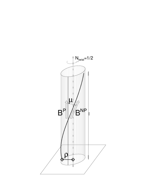
Figure 2.: The basic 3D geometry of a cylindrical flux tube with uniform twist is defined by the length $l$ of the cylinder axis, the number of twisting turns along this length, $N_{\rm twist}$, or by the misalignment angle $\mu$ at the flux tube radius $\rho$ between the potential field line ${\bf B}^{\rm P}$ (aligned with the cylindrical axis) and the non-potential field line ${\bf B}^{\rm NP}$ (aligned with the twisted loop). The non-potential field line ${\bf B}^{\rm NP}$ can be decomposed into a longitudinal field component $B_{s}$ and an azimuthal field component $B_{\varphi}$.

We consider a straight cylinder where a uniform twist is applied, so that an initially straight field line ${\bf B}=(0,0,B_{s})$, aligned with a field line coordinate $s$, is rotated by a number $N_{\rm twist}$ of full turns over the cylinder length $l$, yielding an azimuthal field component $B_{\varphi}$ at radius $\rho$,

$${B_{\varphi}\over B_{s}}={\rho\partial\varphi\over\partial s}={2\pi\rho N_{\rm twist}\over l}=b\rho\ ,$$ (7)

with the constant $b$ defined in terms of the number of full twisting turns $N_{\rm twist}$ over a (loop) length $l$.

The cylindrical geometry of a twisted flux tube is visualized in Figure 2. The longitudinal component of the untwisted magnetic field corresponds to a potential field vector ${\bf B}^{\rm P}$, while the twisted non-potential field line ${\bf B}^{\rm NP}$ has a helical geometry with an angle $\mu$ at a radius $\rho$, which can be described by the longitudinal component $B_{s}$ and the azimuthal component $B_{\varphi}$. The fluxtube can be considered as a sequence of cylinders with radii $\rho$, each one twisted by the same twist angle $\partial\varphi/\partial s=2\pi N_{\rm twist}/l$. For uniform twisting, the magnetic components $B_{\varphi}$ and $B_{s}$ depend only on the radius $\rho$, but not on the length coordinate $s$ or azimuth angle $\varphi$. Thus, the functional dependence in cylindrical coordinates $(\rho,\varphi,s)$ is

$${\bf B}=\left[B_{\rho},B_{\varphi},B_{s}\right]=\left[0,B_{\varphi}(\rho),B_{s}(\rho)\right]\ .$$ (8)

Consequently, the general expression of $\nabla\times{\bf B}$ in cylindrical coordinates,

$${\nabla}\times{\bf B}=\left[{1\over\rho}{\partial B_{s}\over\partial\varphi}-{\partial B_{\varphi}\over\partial s},{\partial B_{\rho}\over\partial s}-{\partial B_{s}\over\partial\rho},{1\over\rho}\left({\partial\over\partial\rho}(\rho B_{\varphi})-{\partial B_{\rho}\over\partial\varphi}\right)\right]\ ,$$ (9)

is simplified with $B_{\rho}=0$ and the sole dependencies of $B_{\varphi}(\rho)$ and $B_{s}(\rho)$ on the radius $\rho$ (Equation (7)), yielding a force-free current density ${\bf j}$ of,

$${\bf j}=\left[j_{\rho},j_{\varphi},j_{s}\right]={c\over 4\pi}({\nabla}\times{\bf B})={c\over 4\pi}\left[0,-{\partial B_{s}\over\partial\rho},{1\over\rho}\left({\partial\over\partial\rho}(\rho B_{\varphi})\right)\right]\ .$$ (10)

Requiring that the Lorentz force is zero for a force-free solution, ${\bf F}={\bf j}\times{\bf B}=0$, we obtain a single non-zero component in the radial $\rho$-direction, since $j_{\rho}=0$ and $B_{\rho}=0$ for the two other components,

$${\bf F}={\bf j}\times{\bf B}=\left[B_{s}j_{\varphi}-B_{\varphi}j_{s},0,0\right]\ ,$$ (11)

yielding a single differential equation for $B_{s}$ and $B_{\varphi}$,

$$B_{s}{dB_{s}\over d\rho}+B_{\varphi}{1\over\rho}{d\over d\rho}(\rho B_{\varphi})=0\ .$$ (12)

By substituting $B_{\varphi}=b\rho B_{s}$ from Equation (7) into Equation (12), this simplifies to,

$${d\over d\rho}\left[(1+b^{2}\rho^{2})B_{s}\right]=0\ .$$ (13)

A solution is found by making the expression inside the derivative to a constant ($B_{0}$), which yields $B_{\varphi}$ and $B_{s}$,

$${\bf B}=\left[B_{\rho},B_{\varphi},B_{s}\right]=\left[0,{B_{0}\ b\rho\over 1+b^{2}\rho^{2}},{B_{0}\over 1+b^{2}\rho^{2}}\right]\ .$$ (14)

[This equation corrects also a misprint in Equation (5.5.8) of Aschwanden (2004; p.216), where a superflous zero component has to be eliminated]. With the definition of the force-free $\alpha$-parameter,

$$(\nabla\times{\bf B})={4\pi\over c}{\bf j}=\alpha(\rho){\bf B}\ ,$$ (15)

we can now verify that the $\alpha$-parameter for a uniformly twisted fluxtube depends only on the radius $\rho$,

$$\alpha(\rho)={2b\over(1+b^{2}\rho^{2})}\ ,$$ (16)

with the constant $b$ defined in terms of the number of full twisting turns $N_{\rm twist}$ over a (loop) length $l$ (see Equation (7)),

$$b={2\pi N_{\rm twist}\over l}\ .$$ (17)

Figure 3.: The field line geometry is shown for an untwisted cylindrical flux tube (left), a twisted cylindrical flux tube (middle), and for a twisted radial field (right), from the side view in the $xz$-plane (top) and from the top view in the $xy$-plane (bottom). The top panels show the longitudinal magnetic field component $B_{s}(\rho)$ and the bottom panels show the azimuthal magnetic field component $B_{\varphi}(\rho,\varphi)$.

The geometry of a twisted flux tube is visualized in Figure 3 (top middle), where the parallel field lines are aligned with the coordinate axis $s$ in the vertical direction, the cross-sectional radius $\rho$ is defined in the direction perpendicular to $s$, and the twist angle $\varphi$ is indicated in the horizontal projection (Figure 3, bottom middle). According to Equations (8) and (14), the variations of the longitudinal $B_{s}(\rho)$ and of the azimuthal component $B_{\varphi}(\rho)$ with radius $\rho$ are,

$$B_{s}(\rho)={B_{0}\over 1+b^{2}\rho^{2}}\ ,$$ (18)

$$B_{\varphi}(\rho)={B_{0}b\rho\over 1+b^{2}\rho^{2}}\ .$$ (19)

These radial dependencies are shown in Figure 4 for different numbers of twist ($N_{\rm twist}=0.5,1.0,1.5$). In the limit of vanishing twist ($N_{\rm twist}=0\mapsto b=0$), we have an untwisted flux tube (Figure 3 left) with a constant longitudinal field $B_{s}(\rho)=B_{0}$ and a vanishing azimuthal component $B_{\varphi}(\rho)=0$. The dependence of the azimuthal field component $B_{\varphi}(\rho)$ and the longitudinal field component $B_{s}(\rho)$ as a function of the radius ${\rho}$ from the twist axis (Figure 4) shows that the longitudinal component falls off monotonically with radius $\rho$, while the azimuthal component increases first for small distances $\rho\ll l$, but falls off at larger distances. Thus, the twisting causes a smaller cross-section of a fluxtube compared with the potential field situation, as widely known (e.g., Klimchuk et al., 2000).

Figure 4.: The dependence of the longitudinal (solid lines) and azimuthal magnetic field component (dashed lines) as a function of the distance $r/l$ from the twist axis field is shown for three different amounts of twist ($N_{\rm twist}=1.5,1.0,0.5$ full turns per loop length $l$).

2.3 Nonlinear Force-Free Field Parameterization

We are now synthesizing the concept of point-like buried magnetic charges that we used to parameterize a potential field (Section 2.1) with the uniformly twisted flux tube concept that represents an exact solution of a nonlinear force-free field (Section 2.2). The geometric difference between the two concepts is the spherical symmetry of a point charge versus the parallel field configuration of an untwisted flux tube. However, we can synthesize the two geometries by considering the parallel field as a far-field approximation of a radial field. In an Euclidean parallel field, the equi-potential surface is a plane perpendicular to the parallel field vector, while a radial field has spherical equi-potential surface. We can make the transformation of a parallel field in cylindrical coordinates $(s,\rho,\varphi)$ into a radial field with spherical coordinates $(r,\theta,\varphi)$ by mapping (see Figure 3),

$$\begin{array}[]{ll}s&\mapsto r\\ \rho&\mapsto r\sin(\theta)\\ \end{array}\ .$$ (20)

This transformation from cylindrical to spherical coordinates preserves the orthogonality of the longitudinal field component $(B_{s}\mapsto B_{r})$ to the equi-potential surface ($s=$const $\mapsto r=$const) and conserves the magnetic flux $\Phi(r)$ along a bundle of field lines with area $A(r)={\rho^{2}(r)}$,

$$\Phi(r)=B(r)A(r)=B(r)\rho^{2}(r)=B(r)r^{2}\sin^{2}{\theta}={\rm const}\ ,$$ (21)

if the longitudinal component $B(r)\propto r^{-2}$ (Equation (1)) decreases quadratically with distance from the magnetic charge. Thus, applying the transformation into spherical coordinates (Equation (20)) and the magnetic flux conservation (Equation (21)) to the straight flux tube solution (Equations (18) and (19)), we can already guess the approximate nonlinear force-free solution in spherical coordinates,

$$B_{r}(r,\theta)\propto r^{-2}{1\over(1+b^{2}r^{2}\sin^{2}{\theta})}\ ,$$ (22)

$$B_{\varphi}(r,\theta)\propto r^{-2}{br\sin{\theta}\over(1+b^{2}r^{2}\sin^{2}{\theta})}\ .$$ (23)

More rigorously, we can derive a nonlinear force-free field solution by writing the divergence-free condition $(\nabla\cdot{\bf B})=0$ and the force-free condition $(\nabla\times{\bf B})=(4\pi/c){\bf j}=\alpha(\rho){\bf B}$ (Equation (15)) of a magnetic field vector ($B_{r},B_{\theta},B_{\varphi})$ in spherical coordinates $(r,\theta,\varphi)$ (with the origin at the location of the magnetic charge and the spherical symmetry axis aligned with the vertical direction to the local solar surface),

$$(\nabla\cdot{\bf B})={1\over r^{2}}{\partial\over\partial r}(r^{2}B_{r})+{1\over r\sin{\theta}}{\partial\over\partial\theta}(B_{\theta}\sin{\theta})+{1\over r\sin{\theta}}{\partial B_{\varphi}\over\partial\varphi}=0\ ,$$ (24)

$$\left[\nabla\times{\bf B}\right]_{r}={1\over r\sin{\theta}}\left[{\partial\over\partial\theta}(B_{\varphi}\sin{\theta})-{\partial B_{\varphi}\over\partial\varphi}\right]=\alpha B_{r}\ ,$$ (25)

$$\left[\nabla\times{\bf B}\right]_{\theta}={1\over r}\left[{1\over\sin{\theta}}{\partial B_{r}\over\partial\varphi}-{\partial\over\partial r}(rB_{\varphi})\right]=\alpha B_{\theta}\ ,$$ (26)

$$\left[\nabla\times{\bf B}\right]_{\varphi}={1\over r}\left[{\partial\over\partial r}(rB_{\theta})-{\partial B_{r}\over\partial\theta}\right]=\alpha B_{\varphi}\ .$$ (27)

For a simple approximative nonlinear force-free solution we require axi-symmetry with no azimuthal dependence ($\partial/\partial\varphi=0$) and neglect components that contribute only to second order ($B_{\theta}\propto[br\sin{\theta}]^{2}\approx 0)$, in analogy to the uniformly twisted flux tubes on cylindrical surfaces (Figure 2). This requirement simplifies Equations (24)–(27) to,

$${1\over r^{2}}{\partial\over\partial r}(r^{2}B_{r})\approx 0\ ,$$ (28)

$${1\over r\sin{\theta}}{\partial\over\partial\theta}(B_{\varphi}\sin\theta)=\alpha B_{r}\ ,$$ (29)

$$-{1\over r}{\partial\over\partial r}(rB_{\varphi})\approx 0\ ,$$ (30)

$$-{1\over r}{\partial B_{r}\over\partial\theta}\approx\alpha B_{\varphi}\ .$$ (31)

Eliminating $\alpha$ from Equations (29) and (31) and using the analog ansatz as for cylindrical fluxtubes (Equation (7)),

$$B_{\varphi}=B_{r}br\sin{\theta}\ ,$$ (32)

we obtain a similar differential equation as in Equation (13),

$${\partial\over\partial\theta}\left[B_{r}(1+b^{2}r^{2}\sin^{2}{\theta})\right]=0\ .$$ (33)

A solution of this differential equation is obtained by setting the expression inside the bracket to the constant $B_{0}(d^{2}/r^{2})$, which fulfills the divergence-free condition (Equation (28)), and we obtain a solution for $B_{r}$ and $B_{\varphi}$ (using Equation (32)), for $\alpha$ (using Equation (29)),

$$B_{r}(r,\theta)=B_{0}\left({d^{2}\over r^{2}}\right){1\over(1+b^{2}r^{2}\sin^{2}{\theta})}\ ,$$ (34)

$$B_{\varphi}(r,\theta)=B_{0}\left({d^{2}\over r^{2}}\right){br\sin{\theta}\over(1+b^{2}r^{2}\sin^{2}{\theta})}\ ,$$ (35)

$$B_{\theta}(r,\theta)\approx 0\ ,$$ (36)

$$\alpha(r,\theta)\approx{2b\cos{\theta}\over(1+b^{2}r^{2}\sin^{2}{\theta})}\ .$$ (37)

This solution fulfills both the force-free condition (Equations (29)–(31)) and the divergence-free condition (Equation (28)) to second-order accuracy ($\propto[br\sin{\theta}]^{2}$). We see that this solution is identical with the simplified derivation of Equations (22) and (23). At locations near the twist axis ($\theta\mapsto 0$), the general solution (Equations (34)–(37)) converges to the cylindrical flux tube geometry solution (Equations (18) and (19)). Furthermore, in the limit of vanishing twist ($b\mapsto 0$) we retrieve the potential-field solution (Equation (4)), since the force-free parameter becomes $\alpha\mapsto 0$, the azimuthal field component becomes $B_{\varphi}=0$, and the radial component reproduces the potential-field solution $B_{r}\mapsto B_{0}(d^{2}/r^{2})$.

Figure 5.: The geometry of a twisted radial field of a magnetic charge $j$ buried at a subphotospheric position $(x_{j},y_{j},z_{j})$ is shown. The central twist axis (dashed line) intersects an equi-potential surface at position $(x_{0},y_{0},z_{0})$ and the longitudinal field vector $B_{r}$ at position $(x,y,z)$ has a radial distance $\rho$ from the twist axis and an azimuth angle $\varphi$. The azimuthal magnetic field component $B_{\varphi}$ at location $(x,y,z)$ is orthogonal to the radial vector ${\rho}$ and the longitudinal field component $B_{r}$, as well as to the direction of the twist axis ${\bf R}$.

2.4 Cartesian Coordinate Transformation

In the derivation in the last section we derived the solution in terms of spherical coordinates $(r,\theta,\varphi)$ in a coordinate system where the rotational symmetry axis is aligned with the vertical to the solar surface intersecting a magnetic charge $j$. Since we are going to model a number of magnetic charges at arbitrary positions on the solar disk, we have to transform an individual coordinate system $(r_{j},\theta_{j},\varphi_{j})$ associated with magnetic charge $j$ into a Cartesian coordinate system $(x,y,z)$ that is given by the observers line-of-sight (in $z$-direction) and the observer’s image coordinate system $(x,y)$ in the plane-of-sky. The variables of the Cartesian coordinate transformation are shown in Figure 5.

The radial magnetic field vector ${\bf B}_{r}$ (which is pointing radially away from a magnetic charge $j$ located in the solar interior at $(x_{j},y_{j},z_{j})$ is simply given by the difference of the Cartesian coordinates from an arbitrary location $(x,y,z)$,

$${{\bf B}_{r}\over B_{r}}=\left[{x-x_{j}\over r_{j}},{y-y_{j}\over r_{j}},{z-z_{j}\over r_{j}}\right]=\left[\cos_{r,x},\cos_{r,y},\cos_{r,z}\right]\ ,$$ (38)

where $B_{r}$ is the absolute value of the radial magnetic field component $B_{r}(r_{j},\theta_{j})$ (Equation (34)), $r_{j}$ is the spatial length of the radial vector ${\bf r}_{j}$ (Equation (3)), defining the directional cosines $\cos_{r,i}$ (for the 3D coordinates $i=x,y,z$) of the radial magnetic field vector ${\bf B}_{r}$.

The azimuthal component ${\bf B}_{\varphi}$ (with the absolute value $B_{\varphi}(r_{j},\theta_{j})$ defined in Equation (35)) of the twisted magnetic field is orthogonal to the direction of the twist axis ${\bf R}$ (aligned with the local vertical),

$${\bf R}=\left[x_{j},y_{j},z_{j}\right]\ ,$$ (39)

and the radial magnetic field component ${\bf B}_{r}$ (Figure 5), and thus can be computed from the vector product of the two vectors ${\bf B}_{r}$ and ${\bf R}$,

$${{\bf B}_{\varphi}\over B_{\varphi}}={{\bf R}\times{{\bf B}_{r}}\over|{\bf R}\times{\bf B}_{r}|}=\left[\cos_{\varphi,x},\cos_{\varphi,y},\cos_{\varphi_{z}}\right]\ ,$$ (40)

which defines the directional cosines $\cos_{\varphi,i}$ of the azimuthal component in the Cartesian coordinate system. The vector product allows us also to extract the inclination angle $\theta_{j}$ between the radial magnetic field component ${\bf B}_{r}$ and the local vertical direction ${\bf R}$,

$$\theta_{j}=\sin^{-1}\left({|{\bf R}\times{\bf B}_{r}|\over|{\bf R}|\ |{\bf B}_{r}|}\right)\ .$$ (41)

Finally, the total non-potential magnetic field vector ${\bf B}=(B_{x},B_{y},B_{z})$ is then the vector sum of the radial ${\bf B}_{r}$ and the azimuthal magnetic field component ${\bf B}_{\varphi}$,

$$\begin{array}[]{ll}B_{x}&=B_{r}(r_{j},\theta_{j})\cos_{r,x}+B_{\varphi}(r_{j},\theta_{j})\cos_{\varphi,x}\\ B_{y}&=B_{r}(r_{j},\theta_{j})\cos_{r,y}+B_{\varphi}(r_{j},\theta_{j})\cos_{\varphi,y}\\ B_{z}&=B_{r}(r_{j},\theta_{j})\cos_{r,z}+B_{\varphi}(r_{j},\theta_{j})\cos_{\varphi,z}\end{array}\ ,$$ (42)

with the directional cosines ($\cos_{r,i}$, $\cos_{\varphi,i}$, $\cos_{\theta,i}$) defined by Equations (38) and (40). This is a convenient parameterization that allows us directly to calculate the magnetic field vector of the non-potential field ${\bf B}_{j}=(B_{x},B_{y},B_{z})$ associated with a magnetic charge $j$ that is characterized with five parameters: $(B_{j},x_{j},y_{j},z_{j},\alpha_{j})$, where we define the force-free $\alpha$-parameter from the twist parameter $b_{j}=2\pi N_{\rm twist}/l$ (Equation (7)) at the location of the twist axis ($\theta_{j}=0$),

$$\alpha_{j}=\alpha(\theta_{j}=0)={2\ b_{j}}\ ,$$ (43)

according to Equation (37).

2.5 Superposition of Twisted Field Components

The total non-potential magnetic field from all $j=1,...,N_{\rm m}$ magnetic charges can be approximately obtained from the vector sum of all components $j$ (in an analog way as we applied in Equation (6) for the potential field),

$${\bf B}({\bf x})=\sum_{j=1}^{N_{\rm m}}{\bf B}_{j}({\bf x})\ ,$$ (44)

where the vector components ${\bf B}_{j}=(B_{x,j},B_{y,j},B_{z,j})$ of the non-potential field of a magnetic charge $j$ are defined in Equation (42), which can be parameterized with $5N_{\rm m}$ free parameters $(B_{j},x_{j},y_{j},z_{j},\alpha_{j})$ for a non-potential field, or with $4N_{\rm m}$ free parameters for a potential field (with $\alpha_{j}=0$). Of course, the sum of force-free magnetic field vectors is generally not force-free, but we will prove in the following (Equations (46) and (47)) that the sum of NLFFF solutions of the form of Equations (34)–(37)), which are force-free to second-order accuracy in $\alpha$ (or, more strictly, in $[br\sin\theta]$), have the property that their sum is also force-free to second-order in $\alpha$.

Let us first consider the condition of divergence-freeness. Since the divergence operator is linear, the superposition of a number of divergence-free fields is divergence-free also,

$$\nabla\cdot{\bf B}=\nabla\cdot(\sum_{j}{\bf B}_{j})=\sum_{j}(\nabla\cdot{\bf B}_{j})=0\ .$$ (45)

While the divergence-free condition is exactly fulfilled for a potential field solution (Equation (4)), our quasi-forcefree approximation (Equations (34)–(37)) matches this requirement to second order in $\alpha$, as the insertion of the solutions (Equations (34)–(37)) into the divergence expression (Equation (24)) shows. For a quantitative measure of this level of accuracy we can also check numerical tests of the figure of merit (Section 3.3).

Now, let us consider the condition of force-freeness. A force-free field has to satisfy Maxwell’s equation (Equation (15)). Since we parameterized both the potential field and the non-potential field with a linear sum of $N_{\rm m}$ magnetic charges, the requirement would be,

$$\nabla\times{\bf B}=\nabla\times\sum_{j=1}^{N_{\rm m}}{\bf B}_{j}=\sum_{j=1}^{N_{\rm m}}(\nabla_{j}\times{\bf B}_{j})=\sum_{j=1}^{N_{\rm m}}\alpha_{j}({\bf r}){\bf B}_{j}=\alpha({\bf r}){\bf B}\ .$$ (46)

Generally, these three equations of the vector ${\nabla\times\bf B}$ cannot be fulfilled with a scalar function $\alpha({\bf r})$ for a sum of force-free field components, unless the magnetic field volume consists of spatially separated force-free subvolumes. However, we can show the validity of the force-freeness equation (Equation (46)) to second-order accuracy in $\alpha$. Note, that the nonlinear force-free parameter $\alpha$ is proportional to $b$ (Equations (37) and (43)), which is defined in Equation (17), and thus we set second-order accuracy in $b$ equal to second-order accuracy in $\alpha$. The argument goes as follows. If we use spherical coordinates, the NLFFF solution of the radial component is of zeroth order, $B_{r}(r,\theta)\propto O(\alpha^{0})$ (Equation (34)), the azimuthal component is of first order, $B_{\varphi}(r,\theta)\propto O(\alpha^{1})$ (Equation (35)), and the neglected third component magnetic field component is of second-order, $B_{\theta}(r,\theta)\propto O(\alpha^{2})$ (as it can be shown by inserting $B_{r}$ and $B_{\varphi}$ into Equation (26). The curl of the magnetic field (Equations (25)–(27)) is then of first order for the radial component, $[\nabla\times{\bf B}]_{r}\propto\alpha B_{r}\propto O(\alpha^{1})$ (Equation (25)), to second order for the azimuthal component, $[\nabla\times{\bf B}]_{\varphi}\propto(\alpha B_{\varphi})\propto O(\alpha^{2})$ (Equation (27)), and the remaining third component is of third-order, $[\nabla\times{\bf B}]_{\theta}\propto(\alpha B_{\theta})\propto O(\alpha^{3})$ (Equation (26)).

Therefore, if we neglect second-order and higher-order terms, the divergence-free condition (Equation (46)), which generally has three equations for the three curl components, e.g., $[\nabla\times B_{r}]_{r}$, $[\nabla\times B_{\varphi}]_{\varphi}$, $[\nabla\times B_{\theta}]_{\theta}$, reduces to one single equation for the radial component, $[\nabla\times B_{r}]_{r}$, which can be fulfilled with a scalar function $\alpha({\bf r})$,

$$\alpha({\bf r})\approx{[\nabla\times{\bf B}]_{r}\over B_{r}}={[\nabla\times\sum_{j=1}^{N_{\rm m}}{\bf B}_{j}]_{r}\over\sum_{j=1}^{N_{\rm m}}{\bf B}_{j,r}}={[\sum_{j=1}^{N_{\rm m}}\nabla\times{\bf B}_{j}]_{r}\over\sum_{j=1}^{N_{\rm m}}{\bf B}_{j,r}}={\sum_{j=1}^{N_{\rm m}}\alpha_{j}B_{j}\over\sum_{j=1}^{N_{\rm m}}B_{j}}\ .$$ (47)

Thus, we expect that the force-freeness is fulfilled to second-order accuracy $O(\alpha^{2})$ (or strictly speaking $O(b^{2})$). We will demonstrate the near force-freeness of simulated examples in the next section.

3 Simulations and Tests

We are now going to simulate examples of the analytical nonlinear force-free solutions in order to visualize the magnetic topology and to quantify the accuracy of the divergence-free and force-free conditions.

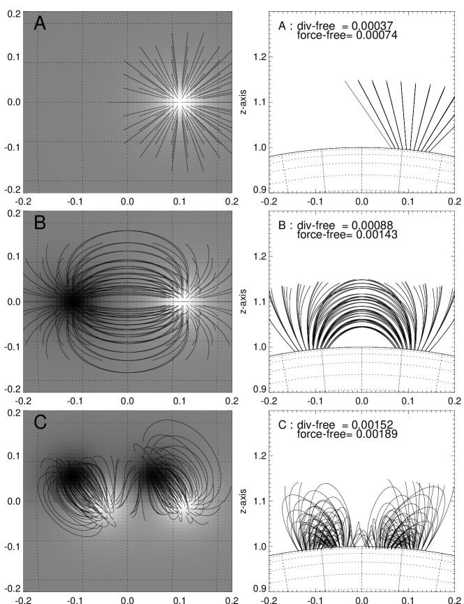
Figure 6.: Simulations of three line-of-sight magnetograms (left) and magnetic field lines projected into the $x-y$ plane (left) and into the vertical $x-z$ plane (right). Thre three cases include: (A) a single positive magnetic charge (first row), (B) a dipole produced by two magnetic charges with opposite polarity (second row), and (C) a quadrupole configuration (third row). See parameters in Table 1. Only field lines with magnetic fields above a 50% threshold of the maximum field strength are shown.

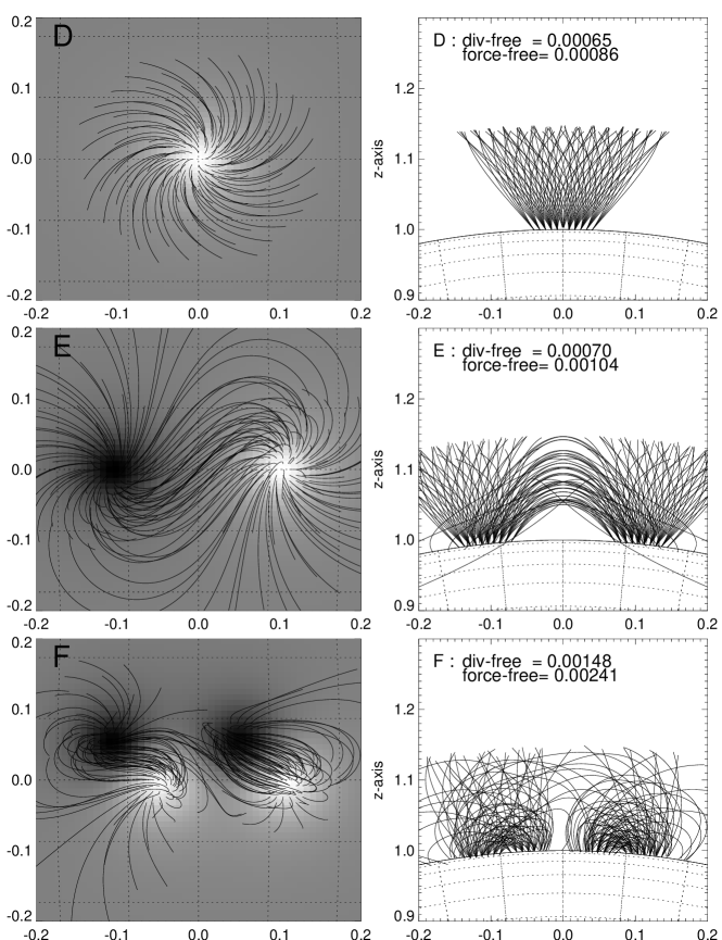
Figure 7.: Simulations of three line-of-sight magnetograms (left) and magnetic field lines of a non-potential model with currents are shown, projected into the $x-y$ plane (left) and into the vertical $x-z$ plane (right). The parameters of the three cases (D), (E), and (F) are identical to thoes of (A), (B), and (C), except for the addition of electric currents.

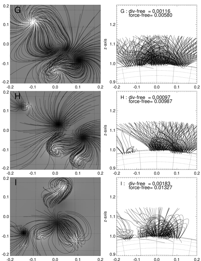
Figure 8.: Simulations of three line-of-sight magnetograms (left) and magnetic field lines of a non-potential model with currents are shown, projected into the $x-y$ plane (left) and into the vertical $x-z$ plane (right). The three cases (G), (H), and (I) have each $N_{\rm m}=10$ magnetic charges, with randomly chosen field strengths, locations, and electric currents.

3.1 Numerical Examples

The simplest case is a single magnetic charge $j=1$, which we illustrate as case A in Figure 6 (top row). We choose the following parameters: a magnetic field strength of $B_{1}=1000$ G (gauss) at the solar surface directly above the buried charge, the location $(x_{1},y_{1},z_{1})=(0.1,0.0,0.95)$ for the buried charge, and a number of zero twist $b_{1}=0$ for the potential field case. We show the simulated line-of-sight magnetogram $B_{z}(x,y)$ in Figure 1 (top left), which mimics an isolated sunspot. The pixel size of the magnetogram and the stepping size in the extrapolation along a field line is $\Delta s=0.004$ solar radii (2800 km $\approx 4\hbox{${}^{\prime\prime}$}$, corresponding to the pixel size of SoHO/MDI magnetograms). We extrapolate the field lines for every pixel that has a footpoint magnetic field strength above a threshold of 50% ($>500$ G). The field lines point in radial direction away from the center of the buried magnetic charge, as it is expected for the potential field of an isolated sunspot (and defined in Equation (1)).

The next basic example is a magnetic dipole, which can be represented in our model by a superposition of a pair of two magnetic charges with opposite polarity, as sketched in Figure 1. The case B shown in Figure 6 is simulated with equal, but oppositely signed magnetic field strengths ($B_{1}=1000$ G, $B_{2}=-1000$ G) at mirrored positions ($x_{1}=0.1,x_{2}=-0.1$), otherwise we used the same parameters as in case A ($y_{1}=y_{2}=0.0,r_{1}=r_{2}=0.95,b_{2}=b_{1}=0.0$). The magnetic field lines mimic the familiar structure of a dipole, which is parameterized here with 8 free parameters (in the potential case).

A quadrupolar configuration is simulated in case C (Figure 6, bottom), with translational symmetry ($x_{1}=0.1,x_{2}=0.05,x_{3}=-0.05,x_{4}=-0.1;y_{1}=0.1,y_{2}=0.05,y_{3}=0.1,y_{4}=0.05$), equal depths ($r_{1}=r_{2}=r_{3}=r_{4}=0.95$), and alternating field strengths ($B_{1}=B_{3}=1000,B_{2}=B_{4}=-1000$ G). The quadrupolar configuration shows essentially two bipoles, each one with field lines that mostly connect within the same dipole domain, but a few intermediate field lines actually connect from one to the other domain.

In Figure 7 we show the same three configurations as for the potential field model (A, B, C of Figure 6), but add electric currents caused by twisting, corresponding to $N_{\rm twist}=-0.5$ turns for the single charge (case D) or first dipole (case E), and $N_{\rm twist}=1.0$ for the second dipole (case F), defined for a loop length of $L=0.1\pi$ solar radii. These amounts of twist correspond to force-free $\alpha$-parameters of $\alpha=2\pi N_{\rm twist}/L=-10$ and $-20$ solar radius^-1 (i.e., $\alpha=-1.43$ and $-2.86\times 10^{-10}$ cm^-1). Comparing the potential (Figure 6) and non-potential cases (Figure 7) shows clearly the differences that result from the presence of electric currents. The force-free field lines of a sunspot become distorted into spiral shapes (case D), the straight dipole becomes distorted into a sigmoid shape (case E), and the quadrupolar configuration becomes also more distorted with sigmoid-like structures (case F).

In Figure 8 we show a few more complicated cases (G, H, and I), consisting of $N_{\rm m}=10$ magnetic charges, with random values chosen in the magnetic field range $-1000$ G $<B_{j}<+1000$ G, in positions $-0.15<x_{j}<0.15$ solar radii, $-0.15<y_{j}<0.15$ solar radii, $0.95<r_{j}<0.97$ solar radii, and random twist in the range $-3<N_{\rm twist}<+3$ per $L=0.1\pi$ solar radii. The field lines displayed in Figure 8 demonstrate that a rich variety of sigmoid-shaped dipoles and inter-connecting multi-pole configurations can be generated with our quasi-force-free solutions, which mimic realistic active regions observed in the solar corona.

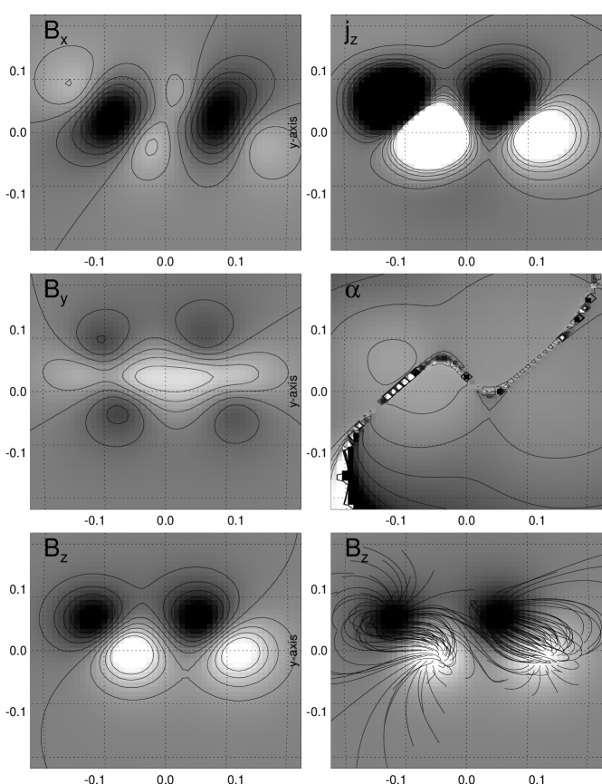
Figure 9.: Maps of the magnetic field components $B_{x}(x,y),B_{y}(x,y),B_{z}(x,y)$ (left panels), the electric current density $j_{z}(x,y)$, and the force-free $\alpha$-parameter (right panels).

3.2 Force-Free $\alpha$-Parameter and Electric Current Maps

In Figure 9 we show examples of various maps that can be generated to visualize a 3D vector field solution, for the case F of a quadrupolar configuration with currents. We show the following quantities in the image plane $(x,y,z=1+\Delta s)$, which corresponds to an image plane near the solar surface: The three magnetic field vector component maps $B_{x}(x,y)$, $B_{y}(x,y)$, $B_{z}(x,y)$ (Figure 9, left panels, the vertical electric current map $j_{z}(x,y)$ (Figure 9, top right panel), the nonlinear $\alpha$-parameter $\alpha(x,y)$ (Figure 9, middle right panel), and the LOS magnetogram $B_{z}(x,y)$ together with extrapolated field lines (Figure 9, bottom right panel). The $B_{z}$ map shows most clearly the locations of the four buried magnetic charges that form two dipolar or a quadrupolar configuration. The magnetic polarization is also reflected in the $j_{z}$ and $\alpha$-map. The $B_{z}$ and the $\alpha$-map show also the location of the neutral line, where numerical effects due to the limited spatial resolution become visible.

Table 1.: Figures of merit for nine simulations of nonlinear force-free field solutions, detailing the size of the 3D datacube, the number of magnetic charges ($N_{\rm m}$), potential or non-potential model (P and NP), the number of computed field lines $N_{\rm f}$, the divergence-freeness $L_{\rm d}$, the force-freeness $L_{\rm f}$, and the computation times $t_{\rm CPU}$.

Case	Data cube	Magnetic	Field	Divergence-	Force-	Computation
		charges	lines	freeness	freeness	time
		$N_{\rm m}$	$N_{\rm f}$	$L_{\rm d}$	$L_{\bf f}$	$t_{\rm CPU}$ (s)
A	$51\times 51\times 37$	1 (P)	87	0.0004	0.0007	0.078
B	$51\times 51\times 37$	2 (P)	160	0.0009	0.0014	0.309
C	$51\times 51\times 37$	4 (P)	159	0.0015	0.0019	0.351
D	$51\times 51\times 37$	1 (NP)	87	0.0006	0.0009	0.083
E	$51\times 51\times 37$	2 (NP)	160	0.0007	0.0010	0.314
F	$51\times 51\times 37$	4 (NP)	159	0.0015	0.0024	0.414
G	$51\times 51\times 37$	10 (NP)	336	0.0012	0.0058	2.462
H	$51\times 51\times 37$	10 (NP)	302	0.0010	0.0099	1.764
I	$51\times 51\times 37$	10 (NP)	217	0.0018	0.0133	1.370

3.3 Figures of Merit

The degree of convergence towards a divergence-free magnetic field model solution can be quantified by a measure that compares the average divergence $\nabla\cdot{\bf B}$, which should be close to zero, with the gradient $B/\Delta x$ of the magnetic field over a reference length scale $\Delta x$, for instance a pixel of the computational grid. The average deviation can then be defined by (see also Wheatland et al., (2000) or Schrijver et al., (2006)),

$$L_{\rm d}={1\over V}\int_{V}{|(\nabla\cdot{\bf B})|^{2}\over|B/\Delta x|^{2}}dV\ .$$ (48)

Similarly, the force-freeness can be quantified by the ratio of the Lorentz force, $({\bf j}\times{\bf B})=(\nabla\times{\bf B})\times{\bf B}$ to the normalization constant $B^{2}/\Delta x$,

$$L_{\rm f}={1\over V}\int_{V}{|(\nabla\times{\bf B})\times{\bf B}|^{2}\over|B^{2}/\Delta x|^{2}}dV\ ,$$ (49)

where $B=|{\bf B}|$.

We calculated these figure of merit quantities for the nine cases simulated in Figures 6-9. The values are listed in each of the panels in Figures 6-8 and listed in Table I. The potential-field cases (A, B, and C) are found to have a figure of merit in the range of $L_{\rm d}=0.0009\pm 0.0006$ for the divergence-freeness, and $L_{\rm f}=0.0014\pm 0.0006$ for the force-freeness. The non-potential field cases (D, E, F, G, H, and I) have values in similar ranges of $L_{\rm d}=0.0009\pm 0.0005$ for the divergence-freeness, and $L_{\rm f}=0.0100\pm 0.0080$ for the force-freeness. We find no tendency that this figure of merit depends on the number of magnetic charges or some other model parameters. The fact that our quasi-force free analytical solutions perform equally well as standard NLFFF codes described in Schrijver eq al. (2006) tells us that the inaccuracy of the analytical approximation is commensurable or even smaller than the numerical uncertainty of other NLFFF codes. However, since our analytical solution provides an explicit formulation of nonlinear force-free fields, it can be computed much faster than the standard NLFFF codes, and still provides approximate solutions with acceptable accuracy (to second order). The computation time of the analytical solutions for the cases shown in Figures 6-8 amounts to about 1 s (on a recent Mac computer: Mac OS X, $2\times 3.2$ GHz Quad-Core Intel Xeon, Memory 32 GB 800 MHz DDR2 FB-DIMM), while standard iterative NLFFF codes need several hours to converge to a single NLFFF solution.

4 Discussion and Conclusions

The coronal magnetic field has generally been computed by extrapolation from lower boundary data in form of photospheric magnetograms $B_{z}(x,y,z=z_{ph})$ or vector-magnetograph data ${\bf B}(x,y)$, using a numerical extrapolation algorithm that fulfills the conditions of force-freeness ($\nabla\cdot{\bf B}$) and divergence-freeness $\nabla\times{\bf B}=\alpha({\bf r}){\bf B}$, where $\alpha({\bf r})$ is a scalar function in space ${\bf r}$. These extrapolation algorithms are very computing-intensive, because a good solution requires many iterations on a large computational 3D-grid that has sufficient spatial resolution to resolve the relevant magnetic field gradients. The accuracy of these numerical solutions depends very much on the noise in boundary vector magnetic field data as well as on deviations of photospheric fields from a force-free state. Recent stereoscopic triangulation of coronal loops has demonstrated a considerable mismatch between the extrapolated fields and the actual coronal loops, which cannot easily be reconciled with extrapolation algorithms, since they have only a very limited degree of freedom within the noise of the boundary data. Moreover, since each NLFFF solution is very time-consuming to compute, these algorithms are not suitable for forward-fitting.

The forward-fitting of magnetic field solutions to observed data requires a faster algorithm to compute many NLFFF solutions for variable boundary data or for coronal constraints as given by stereoscopic 3D reconstructions. The fastest computational way would be an explicit analytical solution for the coronal field vectors ${\bf B}({\bf r})$ as a function of some suitable parameterization of the boundary data or coronal constraints. There exist some analytical solutions of nonlinear force-free fields, such as a class of solutions in terms of Legendre polynomials (Low and Lou, 1990), which is characterized by some spatial symmetry and has been used to test numerical extrapolation algorithms (e.g., DeRosa et al., 2009; Malanushenko et al., 2009). However, to our knowledge, the class of analytical NLFFF solutions of Low and Lou (1990) has never been applied to forward-fitting of observed data, such as line-of-sight magnetograms, vector magnetograph 3D data, or to stereoscopically triangulated loops. Moreover, the special class of NLFFF solutions derived in Low and Lou (1990) correspond to harmonics of Legendre polynomials, which have a high degree of symmetry that does not match realistic observations of active regions, and thus is not suitable for forward-fitting to real data.

What we need to model observed solar magnetic data with high accuracy is: (1) an explicit formulation of an analytical NLFFF solution; (2) a parameterization of the NLFFF solution with a sufficient large number of free parameters that can be forward-fitted to data and converges close to observations; and (3) a fast computation algorithm that can perform many interations without computing-intensive techniques. Hence, such a project consists of developing a suitable analytical formulation first, and then to implement the analytical solutions into a forward-fitting code. In this paper we have undertaken the first step. We started with a potential-field parameterization in terms of $N_{\rm m}$ buried magnetic charges, which is defined by $4N_{\rm m}$ free parameters that can easily be extracted from an observed line-of-sight magnetogram $B_{z}(x,y)$ with arbitrary accuracy, as demonstrated in two recent studies (Aschwanden and Sandman, 2010; Aschwanden et al., 2012a). The key concept of this potential-field representation is that an arbitrary complex 3D magnetic field can be decomposed into a finite number of elementary magnetic field components, where each one simply consists of a quadratically decreasing radial field of a buried magnetic charge. Divergence-freeness is conserved due to the linearity in the superposition of elementary field components. In a next step we extended the elementary potential-field component to a nonpotential-field component by adding a uniform twist that can be parameterized by the force-free $\alpha$-parameter. Such an elementary nonpotential field component requires five free parameters, consisting of the four potential-field parameters plus the force-free $\alpha$-parameter. We derived an explicit analytical formulation of the radial $B_{r}(r,\theta)$ and azimuthal field vector $B_{\varphi}(r,\theta)$ that represents an approximative solution of the divergence-free and force-free condition to second order ($\propto\alpha^{2}$). This solution is very accurate for weakly non-potential fields and converges to the potential field solution for $\alpha=0$. In analogy to the potential-field representation, we represent a general non-potential field solution with a superposition of elementary non-potential field components and prove that the divergence-freeness and force-freeness is conserved to second-order accuracy in our NLFFF approximation.

We calculated some examples of potential and non-potential fields that mimic an isolated sunspot, a dipolar and a quadrupolar configuration, as well as more complex multi-polar configurations. The examples show that the magnetic field of arbitrary complex active regions can be represented with our parameterization. Increasing the force-free $\alpha$-parameter distorts circular field lines into helical and sigmoid-shaped geometries. Our parameterization allows one to compute either field lines (starting from arbitrary locations), 3D datacubes of magnetic field vectors, of maps of the force-free $\alpha$-parameter and electric current $j_{z}$ (Figure 9). We tested the figures of merit for divergence-freeness and force-freeness, which amount to $L_{\rm d}\lower 1.72218pt\hbox{$\;\buildrel<\over{\scriptstyle\sim}\;$}10^{-3}$ and $L_{\rm f}\lower 1.72218pt\hbox{$\;\buildrel<\over{\scriptstyle\sim}\;$}10^{-2}$. The examples demonstrate also the computing speed of this algorithm, which amounts to the order of $\approx 1$ s for a computation grid that encompasses a typical active region with the spatial resolution of MDI. Thus, we envision that a full-fletched forward-fitting code can converge within a few seconds to a few minutes, depending on the number of iterations and number of magnetic field components.

Where do we go from here? The next step is the development of a forward-fitting code that uses the magnetic field parameterization described here (see Paper II). We envision the applications to at least three different sets of constraints, requiring three different versions of forward-fitting codes: (i) line-of-sight magnetograms $B_{z}(x,y)$ and 3D coordinates $[x(s),y(s),z(s)]$ of stereoscopically triangulated loops; (ii) line-of-sight magnetograms $B_{z}(x,y)$ and 2D coordinates $[(x(s),y(s)]$ of traced loops; and (ii) vector-magnetograph data $[B_{x}(x,y)$, $B_{y}(x,y)$, $B_{z}(x,y)]$. The first application requires STEREO data, while the second one can be obtained from any EUV imager (e.g., AIA/SDO, TRACE, EIT/ SOHO). The third application can be conducted with the new HMI/SDO data and is equivalent to other NLFFF extrapolation codes without coronal constraints, while the first two use coronal tracers and alleviate the force-free assumption of photospheric data. We envision that these three applications will reveal insights into a number of crucial questions in a novel way.

There is a large number of physical problems and issues that can be addressed with the anticipated forward-fitting code, such as: (i) The force-freeness of the photosphere; (ii) the accuracy of NLFFF solutions; (iii) the spatial distribution of electric currents in active regions; (iv) the temporal evolution of currents before and during flares; (v) the spatial distribution of current dissipation and coronal heating; (vi) helicity injection; (vii) the 3D geometry of coronal loops which is needed for hydrodynamic modeling; (viii) scaling laws of the volumetric heating function with other physical parameters; (ix) tests of the magnetic field strength inferred from coronal seismology, etc.There exists hardly a phenomenon in the solar corona that can be modeled without the knowledge of the coronal magnetic field.

Appendix A: The Gold-Hoyle Flux Rope

A simple geometry of a force-free field structure is the Gold-Hoyle flux rope (Gold and Hoyle, 1960), which consists of a curved axis with helical field lines curved around the axis (Figure 10). While the stretched version of a flux rope with a straight twist axis has the exact force-free solution of a uniformly twisted flux tube (Section 2.2), the curved version of the Gold-Hoyle flux rope is subject to curvature forces due to the gradient of the magnetic field across the flux rope diameter and has a modified force-free solution.

Figure 10.: Cartoon of Gold-Hoyle flux rope.

Figure 11.: Dipolar field lines with various numbers of twisting turns: $N=0$ (potential field line), stable sigmoid ($N=1$; solid line), and unstable sigmoids ($N=2,...,5$; dashed lines), according to our parameterization of point charges with twisted vertical axes. Note that the limit of large twist numbers does not turn into a Gold-Hoyle flux rope (Figure 10) with our parameterization.

In order to explore the limitations of our force-free field parameterization we attempt here to model such a Gold-Hoyle flux rope. We use the coordinates $(x_{0},0,z_{0})$ and $(-x_{0},0,z_{0}$) with $x_{0}=0.1$ and $z_{0}=0.985$ solar radii (marked with diamonds in Figure 11) and extrapolate field lines $B(s)$ with our method, starting from the apex position $(0,0,z_{a})$ with $z_{a}=1.1$, for a set of six cases with various force-free parameters $\alpha_{1}=\alpha_{2}$, where the $\alpha$’s associated with the twist axis of each buried charge are defined by $\alpha=2\pi N_{\rm twist}/L$, with the loop length $L=2\pi x_{0}=0.314$ and the number of twist turns $N_{\rm twist}=0,1,...,5$ (indicated with $N=0,...,5$ in Figure 11). The case $N=0$ corresponds to the potential field case, yielding a coplanar elliptical loop shape. The case $N=1$ represents a slightly twisted field line that has a sigmoid shape and is a quasi-force-free solution. The cases with $N=2,...,5$ are strongly twisted field lines and may be less force-free, since the neglected $\alpha^{2}$ terms could be significant.

Obviously we cannot reproduce the exact shape of the Gold-Hoyle flux rope as shown in Figure 10 (with about seven twist turns) with our choice of parameterization. The reason lies in the geometric constraints of the twist axis, which is semi-circular in the case of the Gold-Hoyle model, but consists of vertical twist axes in our parameterization. So, this counter-example clearly demonstrates the limitations of our parameterization. Nevertheless, although the cartoon with the Gold-Hoyle geometry is very popular, especially for interplanetary flux ropes and CMEs, it is not clear whether such Gold-Hoyle type geometries are found in loops in the lower corona, and whether the Gold-Hoyle geometry corresponds to an exact force-free solution. It is conceivable that the Sun exerts rotational stress mostly in the photosphere (i.e., rotating sunspots), which propagates in vertical direction along the field lines, but does not necessarily lead to a uniformly twisted circular flux tube as shown in Figure 10, because the magnetic field drops rapidly with $r^{-2}$ with height (for magnetic charges with small sub-photospheric depths), and thus the magnetic stress is not uniformly distributed along a semi-circular potential field line as envisioned in the Gold-Hoyle scenario. However, for a case with a near-constant magnetic field strength $B(s)$ along a potential field line, we would expect a uniform twist as outlined in the Gold-Hoyle case.

On the other side, strongly twisted flux tubes with a twist larger than about 1.25 full turns are unstable due to the kink instability and may erupt, which is another reason why multiply twisted flux tubes are unlikely to be found in active regions. Even Gold and Hoyle (1960) found a critical twist number of $\Phi_{\rm twist}\lower 1.72218pt\hbox{$\;\buildrel<\over{\scriptstyle\sim}\;$}2.49\pi$ $(N_{\rm twist}=\Phi_{\rm twist}/2\pi\lower 1.72218pt\hbox{$\;\buildrel<\over{\scriptstyle\sim}\;$}1.25)$ above which no equilibrium exists, which is also confirmed by recent MHD simulations (e.g., Török and Kliem, 2003). Thus, the Gold and Hoyle flux rope case may not be relevant for modeling magnetic fields in stable active regions. Nevertheless, more general parameterizations could be anticipated in future work, such as twist axes that follow potential field lines, rather than vertical axes, as used in our parameterization to minimize the number of free parameters.

We thank Anny Malanushenko for helpful discussions. Part of the work was supported by NASA contract NNG 04EA00C of the SDO/AIA instrument and the NASA STEREO mission under NRL contract N00173-02-C-2035.

References

Aschwanden, M.J.: 2004, Physics of the Solar Corona. An Introduction, Praxis Publishing Co., Chichester UK, and Springer, Berlin, 216.

Aschwanden, M.J., Wülser, J.P., Nitta, N., Lemen, J.: 2008, Astrophys. J. 679, 827.

Aschwanden, M.J.: 2009, Space Sci. Rev. 149, 31.

Aschwanden, M.J., Sandman, A.W.: 2010, Astronom. J. 140, 723.

Aschwanden, M.J., Wülser, J.P., Nitta, N.V., Lemen, J.R., DeRosa, M., Malanushenko, A.: 2012a, Astrophys. J. , submitted.

Aschwanden, M.J., Wülser, J.P., Nitta, N.V., Lemen, J.R.: 2012b, Solar Phys. , in press.

Aschwanden, M.J., Malanushenko, A.: 2012, Solar Phys. , submitted, (Paper II).

Boyd, T.J.M., Sanderson, J.J.: 2003, The Physics of Plasmas, Cambridge University Press, Cambridge, 102.

Conlon, P.A., Gallagher, P.T.: 2010, Astrophys. J. 715, 59.

DeRosa, M.L., Schrijver, C.J., Barnes, G., Leka, K.D., Lites, B.W., Aschwanden, M.J., et al., : 2009, Astrophys. J. 696, 1780.

Feng, L., Inhester, B., Solanki, S., Wiegelmann, T., Podlipnik, B., Howard, R.A., Wülser, J.P.: 2007, Astrophys. J. Lett. 671, L205.

Gary, A., Alexander, D.: 1999, Solar Phys. 186, 123.

Gold, T., Hoyle, F.: 1960, Mon. Not. Roy. Astron. Soc. 120, 89.

Jackson, J.D.: 1962, Classical Electrodynamics, John Wiley and Sons, Inc., New York, 184.

Klimchuk, J.A., Antiochos, S.K., Norton, D.: 2000, Astrophys. J. 542, 504.

Low, B.C., Lou, Y.Q.: 1990, Astrophys. J. 352, 343.

Malanushenko, A., Longcope, D.W., McKenzie, D.E.: 2009, Astrophys. J. 707, 1044.

Malanushenko, A., Yusuf, M.H., Longcope, D.W.: 2011, Astrophys. J. 736, 97.

Metcalf, T.R., Jiao, L., Uitenbroek, H., McClymont, A.N., Canfield,R.C.: 1995, Astrophys. J. 439, 474.

Priest, E.R.: 1982, Solar Magnetohyrdodynamics, Geophysics and Astrophysics Monographs Volume 21, D. Reidel Publishing Company, Dordrecht, 125.

Ruan, P., Wiegelmann, T., Inhester, B., Neukirch, T., Solanki, S.K., Feng, L.: 2008, Astron. Astrophys. 481, 827.

Sandman, A., Aschwanden, M.J., DeRosa, M., Wülser, J.P., Alexander, D.: 2009, Solar Phys. 259, 1.

Sandman, A.W., Aschwanden, M.J.: 2011, Solar Phys. 270, 503.

Schrijver, C.J., DeRosa, M.L., Metcalf, T.R., Liu, Y., McTiernan, J., Regnier, S., Valori, G., Wheatland, M.S., Wiegelmann, T.: 2006, Solar Phys. 235, 161.

Sturrock, P.A.: 1994, Plasma Physics. – An Introduction to the Theory of Astrophysical, Geophysical and Laboratory Plasmas, Cambridge University Press, Cambridge, 216.

Török, T., Kliem, B.: 2003, Astron. Astrophys. 406, 1043.

Wheatland, M.S., Sturrock, P.A., Roumeliotis, G., 2000, Astrophys. J. 540, 1150.

Wiegelmann, T., Neukirch, T.: 2002, Solar Phys. 208, 233.

Wiegelmann, T., Inhester, B.: 2003, Solar Phys. 214, 287.

Wiegelmann, T., Lagg, A., Solanki, S.K., Inhester, B., Woch, J.: 2005, Astron. Astrophys. 433, 701.

Wiegelmann, T., Inhester, B.: 2006, Solar Phys. 236, 25.