Strong correlation in Kohn-Sham density functional theory

Abstract

We use the exact strong-interaction limit of the Hohenberg-Kohn energy density functional to approximate the exchange-correlation energy of the restricted Kohn-Sham scheme. Our approximation corresponds to a highly non-local density functional whose functional derivative can be easily constructed, thus transforming exactly, in a physically transparent way, an important part of the electron-electron interaction into an effective local one-body potential. We test our approach on quasi-one-dimensional systems, showing that it captures essential features of strong correlation that restricted Kohn-Sham calculations using the currently available approximations cannot describe.

In principle, Kohn-Sham (KS) density functional theory (DFT) Hohenberg and Kohn (1964); Kohn and Sham (1965) should yield the exact ground-state density and energy of any many-electron system, including physical situations in which electronic correlation is very strong, representing them in terms of non-interacting electrons. Currently available approximations for KS DFT, however, fail at properly describing systems approaching the Mott insulating regime Anisimov et al. (1991), the breaking of the chemical bond Grüning et al. (2003); Cohen et al. (2008), and localization in low-density nanodevices Ghosal et al. (2007); Borgh et al. (2005); Abedinpour et al. (2007), to name a few examples (for a recent review, see Cohen et al. (2012)). Artificially breaking the spin (or other) symmetry can mimic some (but not all) strong-correlation effects, at the price of a wrong characterization of several properties and of a partial loosening of the rigorous KS DFT framework.

Indeed, it is very counterintuitive that strongly-correlated systems, in which the electron-electron repulsion plays a prominent role, can be exactly represented in terms of non-interacting electrons. For this reason, several authors Verdozzi (2008); Helbig et al. (2009); Tempel et al. (2009); Teale et al. (2009, 2010); Kurth et al. (2010); Stefanucci and Kurth (2011); Karlsson et al. (2011); Stoudenmire et al. (2012); Bergfield et al. (2012); Ramsden and Godby (2012); Buijse et al. (1989); Filippi et al. (1994); Gritsenko et al. (1995, 1996); Colonna and Savin (1999) have used accurate many-body solutions of prototypical strongly-correlated systems to obtain (by inversion) and characterize the exact non-interacting KS system. The exact properties needed to describe strong correlation in KS DFT have also been set in a transparent framework Cohen et al. (2008); Mori-Sanchez et al. (2009). These works made it all the more evident how difficult it is to find adequate approximations of the exact KS system, so that, albeit theoretically possible, it may seem unrealistic to describe strongly-correlated systems with KS DFT Cohen et al. (2012).

Here, we address this skepticism by showing that the strong-interaction limit of the Hohenberg-Kohn (HK) energy density functional yields approximations capturing strong-correlation effects within the non-interacting restricted self-consistent KS scheme.

The Letter is organized as follows. First, we introduce the formalism, using the strong-interaction limit of the HK functional to transform exactly an important part of the many-body interaction into an effective local one-body potential, in a physically transparent way. We then present pilot self-consistent Kohn-Sham calculations, showing that this potential is indeed able to capture strong-correlation effects way beyond the reach of present KS DFT approximations. As a prototypical example, we look at the “$2k_{F}\to 4k_{F}$” crossover of electrons confined in quasi-one dimension (Q1D). This crossover is entirely due to the dominant particle-particle repulsion that tends to localize the charge density, destroying the non-interacting shell structure, as it happens in many strong-correlation phenomena. The interest of these results goes beyond quasi-one-dimensional systems, because the latter are a valid test lab for three-dimensional DFT, as clearly discussed in Wagner et al. (2012). Our approximation turns out to be qualitatively right, and quantitatively very accurate for the ionization energies, although less accurate for the ground-state density. We thus conclude by discussing the inclusion of higher-order corrections and strategies for extending the self-consistent calculations to two and three dimensions. Hartree (effective) atomic units are used throughout.

Strong-interaction limit– In Hohenberg and Kohn’s formulation Hohenberg and Kohn (1964) the ground-state density and energy of a many-electron system are obtained by minimizing with respect to the density $\rho({\bf r})$ the energy density functional

$$E[\rho]=F[\rho]+\int d{\bf r}\,v_{\rm ext}({\bf r})\,\rho({\bf r}),$$ (1)

where $v_{\rm ext}({\bf r})$ is the external potential and $F[\rho]$ is a universal functional of the density, defined as the minimum of the internal energy (kinetic energy $\hat{T}$ plus electron-electron repulsion $\hat{V}_{ee}$) with respect to all the fermionic wave functions $\Psi$ that yield the density $\rho({\bf r})$ Levy (1979),

$$F[\rho]=\min_{\Psi\to\rho}\langle\Psi|\hat{T}+\hat{V}_{ee}|\Psi\rangle.$$ (2)

To capture the fermionic nature of the electronic density, Kohn and Sham Kohn and Sham (1965) introduced the functional $T_{s}[\rho]$ by minimizing the expectation value of $\hat{T}$ alone over all the fermionic wave functions yielding the given $\rho$ Levy (1979),

$$T_{s}[\rho]=\min_{\Psi\to\rho}\langle\Psi|\hat{T}|\Psi\rangle,$$ (3)

thus introducing a reference non-interacting system with the same density of the physical, interacting, one. The remaining parts of $F[\rho]$, defining the Hartree and exchange-correlation functional, $E_{\rm Hxc}[\rho]\equiv F[\rho]-T_{s}[\rho]$, are approximated.

The strong-interaction limit of $F[\rho]$ is given by the functional $V_{ee}^{\rm SCE}[\rho]$, defined as Seidl (1999); Seidl et al. (1999, 2000a, 2007)

$$V_{ee}^{\rm SCE}[\rho]=\min_{\Psi\to\rho}\langle\Psi|\hat{V}_{ee}|\Psi\rangle,$$ (4)

where the acronym “SCE” stands for “strictly-correlated electrons” Seidl (1999). The functional $V_{ee}^{\rm SCE}[\rho]$ is the minimum of the electronic interaction alone over all the wave functions yielding the given density. It has been first studied in the seminal work of Seidl and coworkers Seidl (1999); Seidl et al. (1999, 2000a), and later formalized and evaluated exactly in Refs. Seidl et al., 2007; Gori-Giorgi and Seidl, 2010; Räsänen et al., 2011; Buttazzo et al., 2012.

More recently, it has been suggested that a “SCE DFT”, in which the functional $F[\rho]$ is decomposed as $F[\rho]=V_{ee}^{\rm SCE}[\rho]+E_{kd}[\rho]$ Gori-Giorgi et al. (2009a); Liu and Burke (2009); Gori-Giorgi and Seidl (2010), and the so-called kinetic-decorrelation energy $E_{kd}[\rho]$ is approximated, could be a complementary alternative to KS DFT for systems in which the electron-electron repulsion largely dominates over the electronic kinetic energy. Indeed, SCE DFT works well for low-density many-particle scenarios Gori-Giorgi et al. (2009a); Gori-Giorgi and Seidl (2010), but it requires that one knows a priori that the system is in the strong-interaction regime, and it fails when the fermionic shell structure plays a role Gori-Giorgi and Seidl (2010). It also misses several appealing features of KS DFT, e.g. the possibility to yield (at least in principle) the exact ionization energy. More generally, orbitals and orbital energies, crucial for chemistry and solid state physics, are totally absent in SCE DFT.

SCE as a functional for KS DFT – To combine the advantages of KS DFT and SCE DFT, here we use the functional $V_{ee}^{\rm SCE}[\rho]$ to approximate $E_{\rm Hxc}[\rho]$,

$$E_{\rm Hxc}[\rho]\approx V_{ee}^{\rm SCE}[\rho].$$ (5)

Equation (5) amounts to approximating the constrained minimization over $\Psi$ in the HK functional (2) with the sum of two constrained minima,

$$\min_{\Psi\to\rho}\langle\Psi|\hat{T}+\hat{V}_{ee}|\Psi\rangle\approx\min_{\Psi\to\rho}\langle\Psi|\hat{T}|\Psi\rangle+\min_{\Psi\to\rho}\langle\Psi|\hat{V}_{ee}|\Psi\rangle.$$ (6)

This new “KS SCE” approach treats both the kinetic energy and the electron-electron repulsion on the same footing. Standard KS DFT emphasizes the non-interacting shell structure, treated accurately through the functional $T_{s}[\rho]$, but it misses the features of strong correlation. SCE DFT is biased towards localized “Wigner-like” structures in the density, missing the fermionic shell structure. Many interesting systems lie in between these two limits, and their complex behavior arises precisely from the competition between the fermionic structure embodied in the kinetic energy and correlation effects due to the electron-electron repulsion. By letting these factors compete in a self-consistent KS procedure, one might be able to get at least a qualitative description of several complex phenomena, amenable to improvement by corrections in the same spirit of standard KS DFT.

General features of KS SCE – First, notice that for a given density $\rho$, the right-hand side of Eq. (6) is always less or equal than the left-hand side. Even if minimizing our energy functional with respect to the density will not yield the exact $\rho$ [as Eq. (6) is an approximation], it is easy to prove that our final total energy is a lower bound to the exact one.

From the scaling properties Levy and Perdew (1985) of $F[\rho]$, $T_{s}[\rho]$ and $V_{ee}^{\rm SCE}[\rho]$ it derives that the approximation of Eq. (6) is accurate both in the weak- and in the strong-interaction limits, while probably less precise in between. By defining, for electrons in $D$ dimensions, $\rho_{\gamma}({\bf r})\equiv\gamma^{D}\rho(\gamma{\bf r})$, where $\gamma\geq 0$, we have $T_{s}[\rho_{\gamma}]=\gamma^{2}T_{s}[\rho]$, $V_{ee}^{\rm SCE}[\rho_{\gamma}]=\gamma V_{ee}^{\rm SCE}[\rho]$ Gori-Giorgi and Seidl (2010), and $F[\rho_{\gamma}]=\gamma^{2}F_{1/\gamma}[\rho]$, where $F_{1/\gamma}[\rho]$ means that the Coulomb coupling constant in $F[\rho]$ is rescaled with $1/\gamma$. It is then easy to see that both sides of Eq. (6) tend to $T_{s}[\rho_{\gamma}]$ when $\gamma\to\infty$ (high density or weak interaction) and to $V_{ee}^{\rm SCE}[\rho_{\gamma}]$ when $\gamma\to 0$ (low density or strong interaction).

Since KS SCE tends to the exact density and energy in the strong-interaction limit, the corresponding KS potential should have the features that are expected for a KS description of strong correlation Helbig et al. (2009); Buijse et al. (1989); Stoudenmire et al. (2012). We discuss first why, physically and mathematically, the SCE potential [Eqs. (7)-(8) below] is expected to have these features, which we then test practically with self-consistent calculations in Q1D.

Physically, the functional $V_{ee}^{\rm SCE}[\rho]$ portrays the strict correlation regime, where the position ${\bf r}$ of one electron determines all the other $N-1$ electronic positions ${\bf r}_{i}$ through the so-called co-motion functions, ${\bf r}_{i}={\bf f}_{i}[\rho]({\bf r})$, some non-local functionals of the density Seidl et al. (2007); Gori-Giorgi et al. (2009b, a); Buttazzo et al. (2012). Therefore, the net repulsion on an electron at position ${\bf r}$ due to the other $N-1$ electrons depends on ${\bf r}$ alone. Its effect can then be exactly represented Seidl et al. (2007); Gori-Giorgi et al. (2009a); Buttazzo et al. (2012) by a local one-body potential ,

$$\nabla\tilde{v}_{\rm SCE}[\rho]({\bf r})=-\sum_{i=2}^{N}\frac{{\bf r}-{\bf f}_{i}[\rho]({\bf r})}{|{\bf r}-{\bf f}_{i}[\rho]({\bf r})|^{3}}.$$ (7)

The physical meaning of Eq. (7) is very transparent: at each position ${\bf r}$, $\nabla\tilde{v}_{\rm SCE}[\rho]({\bf r})$ exerts the same force as the net electron-electron repulsion. We also have Gori-Giorgi et al. (2009a); Buttazzo et al. (2012)

$$\frac{\delta V_{ee}^{\rm SCE}[\rho]}{\delta\rho({\bf r})}=\tilde{v}_{\rm SCE}[\rho]({\bf r}),$$ (8)

so that the approximation of Eq. (5) corresponds to model the exchange-correlation potential $v_{xc}[\rho]({\bf r})$ of KS DFT as $v_{xc}[\rho]({\bf r})\approx\tilde{v}_{\rm SCE}[\rho]({\bf r})-v_{H}[\rho]({\bf r})$, where $v_{H}[\rho]({\bf r})$ is the Hartree potential. The functional $V_{ee}^{\rm SCE}[\rho]$, being essentially a classical repulsion energy, favors localized charge densities. When evaluated with a delocalized density $\rho$, its functional derivative (8) as a function of ${\bf r}$ displays strong variations pushing electrons towards localization. Otherwise said, Eqs. (7)-(8) transfer the effects of strong-correlation into a physically meaningful, effective local potential, expressed as the functional derivative of a rigorous KS density functional.

While KS SCE does not use explicitly the Hartree functional, the correct electrostatics is still captured, since $V_{ee}^{\rm SCE}[\rho]$ is the classical electrostatic minimum in the given density $\rho$. Moreover, the potential $\tilde{v}_{\rm SCE}[\rho]({\bf r})$ stems from a wave function (the SCE one Seidl et al. (2007); Gori-Giorgi et al. (2009b)) and is therefore completely self-interaction free. Similarly, we expect $\tilde{v}_{\rm SCE}[\rho]({\bf r})$ to have a derivative discontinuity that will be analyzed elsewhere Mirtschink et al. .

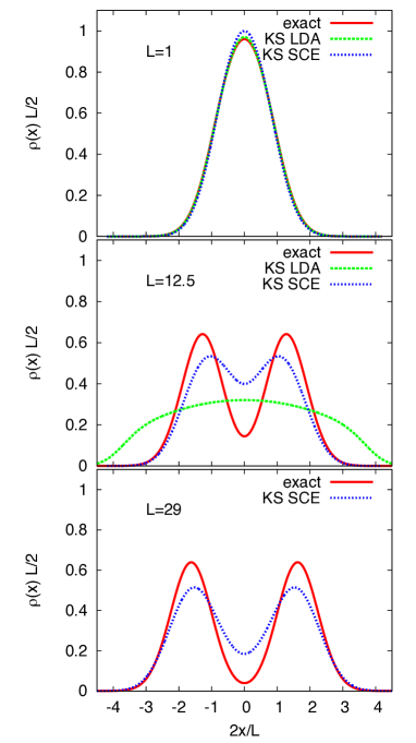
Figure 1: (color online) Self-consistent densities for $N=2$ electrons in Q1D [hamiltonian of Eqs. (9)-(10) with $b=0.1$ and $v_{\rm ext}(x)=\frac{1}{2}\omega^{2}x^{2}$], in units of the effective confinement length $L=2\omega^{-1/2}$ (here and in the following figures). The exact results are compared with KS LDA and KS SCE approximations. At large $L$ the KS LDA calculations do not converge, while KS SCE approaches the exact solution.

Self-consistent KS SCE calculations in Q1D – As a pilot test of the approximation of Eq. (6), we consider $N$ electrons in a thin quantum wire with hamiltonian

$$\hat{H}=-\frac{1}{2}\sum_{i=1}^{N}\frac{\partial^{2}}{\partial x_{i}^{2}}+\sum_{i=1}^{N-1}\sum_{j=i+1}^{N}w_{b}(|x_{i}-x_{j}|)+\sum_{i=1}^{N}v_{\rm ext}(x_{i}),$$ (9)

where the effective Q1D interaction is obtained by integrating the Coulomb repulsion on the lateral degrees of freedom Bednarek et al. (2003),

$$w_{b}(x)=\frac{\sqrt{\pi}}{2\,b}\,\exp\left(\frac{x^{2}}{4\,b^{2}}\right){\rm erfc}\left(\frac{x}{2\,b}\right).$$ (10)

The parameter $b$ fixes the thickness of the wire, and ${\rm erfc}(x)$ is the complementary error function. The interaction $w_{b}(x)$ has a coulombic tail, $w_{b}(x\to\infty)=1/x$, and is finite at the origin, where it has a cusp.

The co-motion functions $f_{i}(x)$ for $N$ electrons can be constructed from the density $\rho(x)$ Seidl (1999); Räsänen et al. (2011); Buttazzo et al. (2012):

$$f_{i}(x)=\Bigg{\{}\begin{array}[]{l}N_{e}^{-1}[N_{e}(x)+i-1]\qquad\qquad\;x\leq a_{N+1-i}\\ N_{e}^{-1}[N_{e}(x)+i-1-N]\qquad x>a_{N+1-i},\end{array}$$ (11)

where the function $N_{e}(x)$ is

$$N_{e}(x)=\int_{-\infty}^{x}\rho(x^{\prime})\,dx^{\prime},$$ (12)

and $a_{k}=N_{e}^{-1}(k)$. Equation (7) becomes in this case

$$\tilde{v}^{\prime}_{\rm SCE}[\rho](x)=\sum_{i=2}^{N}w_{b}^{\prime}(|x-f_{i}(x)|){\rm sgn}(x-f_{i}(x)).$$ (13)

We then solve self-consistently the restricted KS equations in the KS potential $v_{\rm KS}(x)=v_{\rm ext}(x)+\tilde{v}_{\rm SCE}[\rho](x)$, where $\tilde{v}_{\rm SCE}[\rho](x)$ is obtained by integrating Eq. (13) with the boundary condition $\tilde{v}_{\rm SCE}[\rho](|x|\to\infty)=0$.

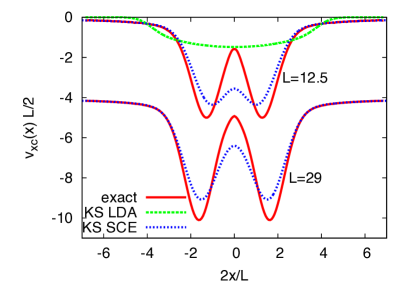
Figure 2: (color online) Self-consistent exchange-correlation potentials for the same system of Fig. 1. For clarity, the potentials for $L=29$ have been shifted by $-4$.

Figure 3: (color online) Self-consistent KS SCE densities for $N=4$ electrons in Q1D [hamiltonian of Eqs. (9)-(10) with $b=0.1$ and $v_{\rm ext}(x)=\frac{1}{2}\omega^{2}x^{2}$].

Here, we aim at showing that this KS SCE approach captures essential features of strong correlation out of reach for standard restricted KS calculations. A simple but very representative example is provided by Abedinpour et. al. Abedinpour et al. (2007), who considered the external harmonic confinement $v_{\rm ext}(x)=\frac{1}{2}\omega^{2}x^{2}$, and performed self-consistent KS calculations within the local density approximation (LDA, Casula et al. (2006)). Fig. 1 shows our results for $N=2$, together with accurate exact values Abedinpour et al. (2007): as expected, KS LDA works well when correlation is weak or moderate, a case characterized by relatively small values of the effective confinement length $L=2\omega^{-1/2}$. As correlation becomes stronger (large $L$), KS LDA cannot describe the “$2k_{F}\to 4k_{F}$” crossover, simply reflected by the doubling of the number of peaks in the density. Indeed, a local or semilocal functional of the density cannot describe this crossover Abedinpour et al. (2007), and exact exchange performs even worse. To localize the charge density, the self-consistent KS potential must build a “bump” (or barrier) between the electrons Abedinpour et al. (2007). This “bump” was discussed in Refs. Buijse et al., 1989 and Helbig et al., 2009: it is expected to be the key feature enabling a KS DFT description of the Mott transition and the breaking of the chemical bond, and it must be a very non-local effect Helbig et al. (2009). We see in Fig. 1 that the self-consistent KS SCE densities, although, as expected, less accurate in between the weak- and the strong-interaction cases, capture the transition to the strongly-correlated regime, thus building, at least partially, the “bump” in the self-consistent KS potential. This is confirmed by the exchange-correlation potentials reported in Fig. 2: we see that the “bump” is clearly present and gets closer to the exact one as the strong-interaction regime is approached. The long-range part of the SCE potential is also remarkably accurate, as expected from the fact that the SCE functional is self-interaction free. Fig. 3 displays the KS SCE densities for $N=4$ electrons: again, we clearly see the crossover from two peaks (the non-interacting shell structure) to four peaks (charge localization).

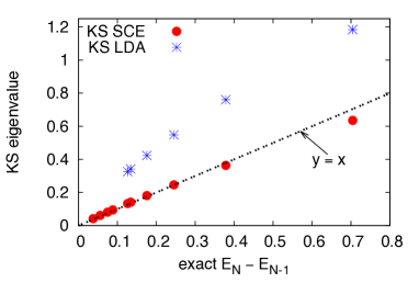
Figure 4: (color online) The KS eigenvalue obtained in the self-consistent KS LDA and KS SCE calculations for the same $N=2$ electron problem considered in Fig. 1, plotted against the negative of the exact ionization energy, $E_{N}-E_{N-1}$.

In the exact KS theory, the highest occupied KS eigenvalue is equal to minus the exact ionization potential $I_{0}=E_{N-1}-E_{N}$ Almbladh and von Barth (1985); Levy et al. (1984). In Fig. 4 we plot the KS LDA and KS SCE eigenvalues for $N=2$, as a function of the exact difference $E_{N}-E_{N-1}$ for several harmonic confinement strengths. We see that KS SCE is remarkably accurate .

Conclusions and Perspectives – The exact strong-interaction limit has the promise of extending KS DFT applicability to strongly-correlated systems, while retaining the appealing properties of the Kohn-Sham approach. In Q1D the computational cost of KS SCE compares to KS LDA. Crucial for future applications is calculating $V_{ee}^{\rm SCE}[\rho]$ and $\tilde{v}_{\rm SCE}[\rho]({\bf r})$ also for general two- and three-dimensional systems. An enticing route towards this goal involves the mass-transportation-theory reformulation of the SCE functional Buttazzo et al. (2012), in which $V_{ee}^{\rm SCE}[\rho]$ is given by the maximum of the Kantorovich dual problem,

$$\max_{u}\left\{\int u({\bf r})\rho({\bf r})d{\bf r}\ :\ \sum_{i=1}^{N}u({\bf r}_{i})\leq\sum_{i=1}^{N-1}\sum_{j>i}^{N}\frac{1}{|{\bf r}_{i}-{\bf r}_{j}|}\right\},$$

where $u({\bf r})=\tilde{v}_{\rm SCE}[\rho]({\bf r})+C$, and $C$ is a constant Buttazzo et al. (2012). This is a maximization under linear constraints that yields in one shot the functional and its functional derivative, and can also inspire approximate and simplified approaches to the construction of $V_{ee}^{\rm SCE}[\rho]$ and $\tilde{v}_{\rm SCE}[\rho]({\bf r})$ Mendl and Lin , a critical step for the computational cost of KS SCE. Another important issue is to add corrections to Eq. (5). One can, more generally, decompose $F[\rho]$ as

$$F[\rho]=T_{s}[\rho]+V_{ee}^{\rm SCE}[\rho]+T_{c}[\rho]+V_{ee}^{d}[\rho],$$ (14)

where $T_{c}[\rho]$ (kinetic correlation energy) is the difference between the true kinetic energy and $T_{s}[\rho]$, and $V_{ee}^{d}[\rho]$ (electron-electron decorrelation energy) is the difference between the true expectation of $\hat{V}_{ee}$ and $V_{ee}^{\rm SCE}[\rho]$. A “first-order” approximation for $T_{c}[\rho]+V_{ee}^{d}[\rho]$ can be, in principle, included exactly using the formalism developed in Ref. Gori-Giorgi et al., 2009b, but other approximations, e.g. in the spirit of Ref. Seidl et al., 2000b, can also be constructed.

Acknowledgments – We thank J. Lorenzana and V. Brosco for inspiring discussions, and K. J. H. Giesbertz, A. Mirtschink, M. Seidl, and G. Vignale for critical readings of the manuscript. This work was supported by the Netherlands Organization for Scientific Research (NWO) through a Vidi grant.

References

- Hohenberg and Kohn (1964) P. Hohenberg and W. Kohn, Phys. Rev. 136, B 864 (1964).
- Kohn and Sham (1965) W. Kohn and L. J. Sham, Phys. Rev. A 140, 1133 (1965).
- Anisimov et al. (1991) V. I. Anisimov, J. Zaanen, and O. K. Andersen, Phys. Rev. B 44, 943 (1991).
- Grüning et al. (2003) M. Grüning, O. V. Gritsenko, and E. J. Baerends, J. Chem. Phys. 118, 7183 (2003).
- Cohen et al. (2008) A. J. Cohen, P. Mori-Sanchez, and W. T. Yang, Science 321, 792 (2008).
- Ghosal et al. (2007) A. Ghosal, A. D. Guclu, C. J. Umrigar, D. Ullmo, and H. U. Baranger, Phys. Rev. B 76, 085341 (2007).
- Borgh et al. (2005) M. Borgh, M. Toreblad, M. Koskinen, M. Manninen, S. Aberg, and S. M. Reimann, Int. J. Quantum Chem. 105, 817 (2005).
- Abedinpour et al. (2007) S. H. Abedinpour, M. Polini, G. Xianlong, and M. P. Tosi, Eur. Phys. J. B 56, 127 (2007).
- Cohen et al. (2012) A. J. Cohen, P. Mori-Sánchez, and W. Yang, Chem. Rev. 112, 289 (2012).
- Verdozzi (2008) C. Verdozzi, Phys. Rev. Lett. 101, 166401 (2008).
- Helbig et al. (2009) N. Helbig, I. V. Tokatly, and A. Rubio, J. Chem. Phys. 131, 224105 (2009).
- Tempel et al. (2009) D. G. Tempel, T. J. Martínez, and N. T. Maitra, J. Chem. Theory Comput. 5, 770 (2009).
- Teale et al. (2009) A. M. Teale, S. Coriani, and T. Helgaker, J. Chem. Phys. 130, 104111 (2009).
- Teale et al. (2010) A. M. Teale, S. Coriani, and T. Helgaker, J. Chem. Phys. 132, 164115 (2010).
- Kurth et al. (2010) S. Kurth, G. Stefanucci, E. Khosravi, C. Verdozzi, and E. K. U. Gross, Phys. Rev. Lett. 104, 236801 (2010).
- Stefanucci and Kurth (2011) G. Stefanucci and S. Kurth, Phys. Rev. Lett. 107, 216401 (2011).
- Karlsson et al. (2011) D. Karlsson, A. Privitera, and C. Verdozzi, Phys. Rev. Lett. 106, 166401 (2011).
- Stoudenmire et al. (2012) E. Stoudenmire, L. O. Wagner, S. R. White, and K. Burke, Phys. Rev. Lett. 109, 056402 (2012).
- Bergfield et al. (2012) J. P. Bergfield, Z.-F. Liu, K. Burke, and C. A. Stafford, Phys. Rev. Lett. 108, 066801 (2012).
- Ramsden and Godby (2012) J. D. Ramsden and R. W. Godby, Phys. Rev. Lett. 109, 036402 (2012).
- Buijse et al. (1989) M. A. Buijse, E. J. Baerends, and J. G. Snijders, Phys. Rev. A 40, 4190 (1989).
- Filippi et al. (1994) C. Filippi, C. J. Umrigar, and M. Taut, J. Chem. Phys. 100, 1290 (1994).
- Gritsenko et al. (1995) O. V. Gritsenko, R. van Leeuwen, and E. J. Baerends, Phys. Rev. A 52, 1870 (1995).
- Gritsenko et al. (1996) O. V. Gritsenko, R. van Leeuwen, and E. J. Baerends, J. Chem. Phys. 104, 8535 (1996).
- Colonna and Savin (1999) F. Colonna and A. Savin, J. Chem. Phys. 110, 2828 (1999).
- Mori-Sanchez et al. (2009) P. Mori-Sanchez, A. J. Cohen, and W. T. Yang, Phys. Rev. Lett. 102, 066403 (2009).
- Wagner et al. (2012) L. O. Wagner, E. M. Stoudenmire, K. Burke, and S. R. White, Phys. Chem. Chem. Phys. 14, 8581 (2012).
- Levy (1979) M. Levy, Proc. Natl. Acad. Sci. U.S.A. 76, 6062 (1979).
- Seidl (1999) M. Seidl, Phys. Rev. A 60, 4387 (1999).
- Seidl et al. (1999) M. Seidl, J. P. Perdew, and M. Levy, Phys. Rev. A 59, 51 (1999).
- Seidl et al. (2000a) M. Seidl, J. P. Perdew, and S. Kurth, Phys. Rev. Lett. 84, 5070 (2000a).
- Seidl et al. (2007) M. Seidl, P. Gori-Giorgi, and A. Savin, Phys. Rev. A 75, 042511 (2007).
- Gori-Giorgi and Seidl (2010) P. Gori-Giorgi and M. Seidl, Phys. Chem. Chem. Phys. 12, 14405 (2010).
- Räsänen et al. (2011) E. Räsänen, M. Seidl, and P. Gori-Giorgi, Phys. Rev. B 83, 195111 (2011).
- Buttazzo et al. (2012) G. Buttazzo, L. De Pascale, and P. Gori-Giorgi, Phys. Rev. A 85, 062502 (2012).
- Gori-Giorgi et al. (2009a) P. Gori-Giorgi, M. Seidl, and G. Vignale, Phys. Rev. Lett. 103, 166402 (2009a).
- Liu and Burke (2009) Z. F. Liu and K. Burke, J. Chem. Phys. 131, 124124 (2009).
- Levy and Perdew (1985) M. Levy and J. P. Perdew, Phys. Rev. A 32, 2010 (1985).
- Gori-Giorgi et al. (2009b) P. Gori-Giorgi, G. Vignale, and M. Seidl, J. Chem. Theory Comput. 5, 743 (2009b).
- (40) A. Mirtschink, M. Seidl, and P. Gori-Giorgi, in preparation.
- Bednarek et al. (2003) S. Bednarek, B. Szafran, T. Chwiej, and J. Adamowski, Phys. Rev. B 68, 045328 (2003).
- Casula et al. (2006) M. Casula, S. Sorella, and G. Senatore, Phys. Rev. B 74, 245427 (2006).
- Almbladh and von Barth (1985) C.-O. Almbladh and U. von Barth, Phys. Rev. B 31, 3231 (1985).
- Levy et al. (1984) M. Levy, J. P. Perdew, and V. Sahni, Phys. Rev. A 30, 2745 (1984).
- (45) C. B. Mendl and L. Lin, arXiv:1210.7117.
- Seidl et al. (2000b) M. Seidl, J. P. Perdew, and S. Kurth, Phys. Rev. A 62, 012502 (2000b).