Tolman’s law in linear irreversible thermodynamics: a kinetic theory approach

Abstract

In this paper it is shown that Tolman’s law can be derived from relativistic kinetic theory applied to a simple fluid in a BGK-like approximation. Using this framework, it becomes clear that the contribution of the gravitational field can be viewed as a cross effect that resembles the so-called Thomson effect in irreversible thermodynamics. A proper generalization of Tolman’s law in an inhomogeneous medium is formally established based on these grounds.

¹,³ Depto. de Fisica y Matematicas, Universidad Iberoamericana, Prolongacion Paseo de la Reforma 880, Mexico D. F. 01219, Mexico.

²Depto. de Matematicas Aplicadas y Sistemas, Universidad Autonoma Metropolitana-Cuajimalpa, Artificios 40 Mexico D.F. 01120, Mexico.

PACS: 47.45.Ab, 04.20.-q, 05.60.-k, 44.10.+i.

Keywords: Tolman’s law, Transport Procceses, Cross-effects, Relativistic gases.

1 Introduction

In 1930 Richard C. Tolman showed that thermal equilibrium can persist within a temperature gradient provided that a gravitational field is present, satisfying the relation:

$$\frac{1}{T}\frac{dT}{dr}=-\frac{g}{c^{2}}$$ (1)

which is often referred to as Tolman´s law [1]. Later, in 1940, Eckart proposed that the heat flux in a special relativistic fluid should be proportional to the temperature gradient and to the hydrodynamic acceleration of the fluid [2]. The corresponding constitutive equation, derived from phenomenological arguments reads

$$J_{\left[Q\right]}^{\mu}=-h^{\mu\nu}\kappa_{T}\left(T_{,\nu}+\frac{T}{c^{2}}a_{\nu}\right)$$ (2)

where $h^{\mu\nu}$ is the spatial projector given by

$$h^{\mu\nu}=g^{\mu\nu}+\frac{1}{c^{2}}\mathcal{U}^{\mu}\mathcal{U}^{\nu}$$ (3)

with $\mathcal{U}^{\mu}$ being the hydrodynamic four-velocity, $\mathcal{U}^{\mu}\mathcal{U_{\mu}}=-c^{2}$ and $\kappa_{T}$ is the thermal conductivity. It seems attractive to relate Eckart´s constitutive equation to Tolman´s law since requiring a vanishing heat flux for equilibrium leads to

$$\frac{1}{T}\frac{\partial T}{\partial x^{\ell}}=-\frac{a_{\ell}}{c^{2}}$$ (4)

which strongly resembles Eq. (1). However, in the presence of stresses the hydrodynamic (macroscopic) acceleration is not equal to gravity. Moreover, the coupling expressed by Eq. (2) does not relate a thermodynamic flux with a canonical force, since $a_{\nu}$ is not the spatial gradient of a state variable as required by irreversible thermodynamics. Also, this coupling has been proven to be the cause of generic instabilities, first identified by Hiscock and Lindblom in 1985 [3][4].

On the other hand, it is well known that kinetic theory provides a framework in which constitutive equations can be established from first principles, in complete consistency with linear irreversible thermodynamics in the Navier-Stokes regime. In this paper, it is shown that a non-vanishing contribution to the heat flux due to a classical gravitational field arises within the framework of relativistic kinetic theory. Such effect strongly resembles the Thomson effect present in plasmas under the influence of an electrostatic field. It becomes equivalent to Tolman’s law for a homogeneous medium at mild temperatures in the presence of a gravitational field.

In section 2 the basic principles of general relativistic kinetic theory within the BGK approximation are described. Section 3 is devoted to the solution of Boltzmann’s equation and to the formal expression for the heat flux, in the presence of a gravitational field, using the Chapman-Enskog expansion to first order in the gradients. In section 4, the corresponding transport coefficient is calculated showing that Tolman’s law follows by requiring a vanishing heat flux in a homogeneous medium. A proper generalization of Tolman’s law in an inhomogeneous medium is also formally established. Conclusions and final remarks are included in section 5.

2 Relativistic kinetic theory

The standard method for establishing transport equations as well as constitutive relations for dissipative fluxes is well known, and has been thoroughly discussed by several authors. The formalism has been successful in many applications, including relativistic fluids [5, 6, 7]. In such program a collisional term for the kinetic equation must be specified as a starting point. In a relaxation time approximation, using the so-called BGK collision kernel for the relativistic gas proposed by Marle [5], the kinetic equation reads

$$v^{\alpha}f_{,\alpha}+a^{\mu}\frac{\partial f}{\partial v^{\mu}}=-\frac{f-f^{\left(0\right)}}{\tau},$$ (5)

where $f$ is the single particle distribution function, $f^{\left(0\right)}$ the local equilibrium (Juttner) distribution [5, 6], $v^{\mu}$ is the molecular four-velocity and $\tau$ is a parameter of the order of the collisional time. Since molecules follow geodetic trajectories, the molecular acceleration $a^{\mu}$ can be written in terms of the curvature induced by a gravitational field as

$$a^{\mu}=-\Gamma_{\alpha\beta}^{\mu}v^{\alpha}v^{\beta}$$ (6)

Thus, Eq. (5) becomes

$$v^{\alpha}f_{,\alpha}-\Gamma_{\alpha\beta}^{\mu}v^{\alpha}v^{\beta}\frac{\partial f}{\partial v^{\mu}}=-\frac{f-f^{\left(0\right)}}{\tau},$$ (7)

According to the Chapman-Enskog method, it is possible to establish a formal solution to the Boltzmann equation in the Navier-Stokes regime that reads:

$$f=f^{(0)}+f^{(1)}$$ (8)

where $f^{\left(1\right)}$ is a correction to local equilibrium to first order in the gradients. Substituting expression (8) in Eq. (7), and retaining only first order terms in the gradients leads to

$$f^{\left(1\right)}=-\tau\left\{v^{\alpha}f_{,\alpha}^{\left(0\right)}-\Gamma_{\alpha\beta}^{\mu}v^{\alpha}v^{\beta}\frac{\partial f^{\left(0\right)}}{\partial v^{\mu}}\right\}$$ (9)

Using the local equilibrium hypothesis, we can write the derivatives of $f^{\left(0\right)}$ in Eq. (9) as:

$$f_{,\alpha}^{\left(0\right)}=\frac{\partial f^{\left(0\right)}}{\partial T}T_{,\alpha}+\frac{\partial f^{\left(0\right)}}{\partial n}n_{,\alpha}+\frac{\partial f^{\left(0\right)}}{\partial\mathcal{U}^{\mu}}\mathcal{U}_{;\alpha}^{\mu}$$ (10)

where $T$ is the local temperature and $n$ is the local number density. Recalling that the Juttner function reads:

$$f^{(0)}=\frac{n}{4\pi c^{3}z\mathcal{K}_{2}\left(\frac{1}{z}\right)}\exp\left(\frac{\mathcal{U}^{\beta}v_{\beta}}{zc^{2}}\right)$$ (11)

a direct calculation leads to

$$f_{,\alpha}^{\left(0\right)}=f^{\left(0\right)}\left\{\frac{n_{,\alpha}}{n}-\left[1-\frac{\gamma}{z}+\frac{1}{2z}\left(\frac{K_{1}\left(\frac{1}{z}\right)}{K_{2}\left(\frac{1}{z}\right)}+\mathcal{G}\left(\frac{1}{z}\right)\right)\right]\frac{T_{,\alpha}}{T}+\frac{v_{\mu}}{zc^{2}}\mathcal{U}_{;\alpha}^{\mu}\right\}$$ (12)

where $K_{n}\left(\frac{1}{z}\right)$ is the $n_{th}$ modified Bessel function of the second kind, $\mathcal{G}\left(\frac{1}{z}\right)=\frac{K_{3}(\frac{1}{z})}{K_{2}(\frac{1}{z})}$ and $\gamma=\gamma_{(k)}$ is the standard Lorentz factor for the molecules’ chaotic velocity $k^{\ell}$ (for more details see Ref.[7]).

Since the molecular four-velocity that appears in Eqs. (11-12) can be written as

$$v^{\alpha}=v_{\mu}h^{\mu\alpha}+\gamma_{\left(k\right)}\mathcal{U}^{\alpha}$$ (13)

the first term of Eq. (9) can be expressed as

$$v^{\alpha}f_{,\alpha}^{\left(0\right)}=v_{\mu}h^{\mu\alpha}f_{,\alpha}^{\left(0\right)}+\gamma_{\left(k\right)}\mathcal{U}^{\alpha}f_{,\alpha}^{\left(0\right)}$$ (14)

or

$$v^{\alpha}f_{,\alpha}^{\left(0\right)} = f^{\left(0\right)}v_{\mu}h^{\mu\alpha}\left\{\frac{n_{,\alpha}}{n}-\left[1-\frac{\gamma}{z}+\frac{1}{2z}\left(\frac{K_{1}\left(\frac{1}{z}\right)}{K_{2}\left(\frac{1}{z}\right)}+\mathcal{G}\left(\frac{1}{z}\right)\right)\right]\frac{T_{,\alpha}}{T}\right.$$ (15)

$$\left.+\frac{v_{\mu}}{zc^{2}}\mathcal{U}_{;\alpha}^{\mu}\right\}+\gamma_{\left(k\right)}\left\{\frac{1}{n}\left.\frac{\partial n}{\partial t}\right|_{CF}+\frac{v_{\mu}}{zc^{2}}\left.\frac{\partial\mathcal{U}^{\mu}}{\partial t}\right|_{CF}\right.$$

$$\left.-\left[1-\frac{\gamma}{z}+\frac{1}{2z}\left(\frac{K_{1}\left(\frac{1}{z}\right)}{K_{2}\left(\frac{1}{z}\right)}+\mathcal{G}\left(\frac{1}{z}\right)\right)\right]\frac{1}{T}\left.\frac{\partial T}{\partial t}\right|_{CF}\right\}$$

where $\left.\frac{\partial}{\partial t}\right|_{CF}$ indicates a derivative calculated in the comoving frame, where locally $\mathcal{U}^{\nu}=\left[0,c\right]$. Following Hilbert’s standard procedure [8], Euler equations are now used in order to express the time derivatives in Eq. (15) in terms of the gradients. We recall that Euler’s equations in the comoving frame read (see Ref. [5]):

$$\left.\frac{\partial n}{\partial t}\right|_{CF}=-n\theta$$ (16)

$$\left.\frac{\partial\mathcal{U}^{\ell}}{\partial t}\right|_{CF}=-\frac{1}{\tilde{\rho}}\left[h^{\ell\nu}\left(\frac{T_{,\nu}}{T}+\frac{n_{,\nu}}{n}\right)-c^{2}\Gamma_{44}^{\ell}\right]\qquad\left.\frac{\partial\mathcal{U}^{4}}{\partial t}\right|_{CF}=0$$ (17)

$$\left.\frac{\partial T}{\partial t}\right|_{CF}=0$$ (18)

In Eq. (17) use has been made of the fact that all four components of the projector $h^{\mu\nu}$ vanish as well as $\Gamma_{44}^{4}$ in a static metric.

The last term of Eq. (9) is easily established, and for a newtonian metric reads:

$$a^{\mu}\frac{\partial f^{(0)}}{\partial v^{\mu}}=-\Gamma_{\alpha\beta}^{\mu}v^{\alpha}v^{\beta}\frac{\mathcal{U}_{\mu}}{zc^{2}}f^{(0)}\simeq-\Gamma_{44}^{\mu}\frac{\mathcal{U}_{\mu}}{z}f^{(0)}$$ (19)

We are now in position to address the main task of this work namely, to analyze the heat flux associated to a gravitational field applied to a simple fluid.

3 Heat flux

In this section attention will only be paid to the gravitational terms present in the first order in the gradients correction to the equilibrium distribution function. Introducing Eqs. (15) to (19) in Eq. (9) and ignoring all terms related to non-gravitational potential gradients one obtains

$$f_{[g]}^{\left(1\right)}=-\tau\frac{1}{zc^{2}}f^{\left(0\right)}\left\{\gamma_{\left(k\right)}v_{\mu}\frac{nm}{\tilde{\rho}}(-\Gamma_{44}^{\mu})+v_{\mu}(\Gamma_{44}^{\mu})\right\},$$ (20)

where $\tilde{\rho}=\frac{n\varepsilon}{c^{2}}+\frac{p}{c^{2}}.$ This expression clearly vanishes in the non-relativistic limit and thus no heat flux is induced due to a gravitational field in a simple non-relativistic fluid, as expected. However, in the relativistic case and using the newtonian approximation for the metric, the following expression can be written:

$$v_{\mu}\Gamma_{44}^{\mu}\simeq\gamma_{\left(k\right)}k_{\ell}\frac{g^{\ell}}{c^{2}}$$

and thus

$$f_{[g]}^{\left(1\right)}=-\tau f^{\left(0\right)}\gamma_{\left(k\right)}\frac{k_{\ell}g^{\ell}}{zc^{2}}\left\{\frac{\gamma_{\left(k\right)}}{\mathcal{G}\left(\frac{1}{z}\right)}-1\right\}$$ (21)

We now recall that the local heat flux in a relativistic fluid is expressed in the Navier-Stokes regime as [9]:

$$J_{\left[Q\right]}^{\ell}=mc^{2}\int k^{\ell}f^{\left(1\right)}\gamma_{\left(k\right)}^{2}d^{*}K$$ (22)

so that the thermal dissipation term that arises from a gradient in the gravitational potential can be identified as:

$$J_{\left[Q,g\right]}^{\ell}=-\tau m\frac{1}{3}g^{\ell}\int f^{\left(0\right)}k^{2}\gamma_{\left(k\right)}^{3}\frac{1}{z}\left\{\frac{\gamma_{\left(k\right)}}{\mathcal{G}\left(\frac{1}{z}\right)}-1\right\}d^{*}K,$$ (23)

Notice that the determinant of the metric is not included as a factor in the integral since within this approximation deviations from a unitary value are second order and higher in the gravitational potential gradient. The invariant velocity volume element $d^{*}K$ is established in Refs.[10, 11]. Details on the procedure to evaluate this type of integrals can also be found in these references. The constitutive equation for the gravitational term in the heat flux can then be written as

$$J_{\left[Q,g\right]}^{\ell}=-L_{Tg}g^{\ell}$$ (24)

where

$$L_{Tg}=\frac{nkT}{z}\tau\left\{5z+\frac{1}{\mathcal{G}\left(\frac{1}{z}\right)}-\mathcal{G}\left(\frac{1}{z}\right)\right\},$$ (25)

The behavior of $L_{Tg}$ can be observed in Fig. 1 where $f_{g}\left(z\right)=L_{Tg}/(kT\tau n)$ is plotted as a function of $z$.

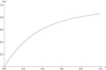
Figure 1: Dependence with $z$ of the coefficient that couples the heat flux with the gravitational field. The coefficient tends to zero in the small $z$, non-relativistic, limit and asymptotes to a constant value for $z\gg 1$ (ultra-relativistic systems).

To the authors’ knowledge this calculation is novel. In the next section we shall analyze the low temperature limit of Eq. (24) and relate the corresponding result to Tolman’s law.

4 Transport coefficients and Tolman’s law

For $z\ll 1$, the expansion in Taylor series of the expression in brackets in Eq. (25) reads:

$$5z+\frac{1}{\mathcal{G}\left(\frac{1}{z}\right)}-\mathcal{G}\left(\frac{1}{z}\right)\sim\frac{5}{2}\left(z^{2}-z^{3}+...\right)$$ (26)

and to lowest order in $z$ one obtains

$$J_{\left[Q,g\right]}^{\ell}\sim-\frac{5}{2}\frac{nk^{2}T^{2}}{mc^{2}}\tau g^{\ell}$$ (27)

If the fluid is assumed to be homogeneous (constant density), the heat flux is expressed as follows:

$$J_{\left[Q\right]}^{\ell}=-L_{TT}\frac{T^{,\ell}}{T}-L_{Tg}g^{\ell},$$ (28)

where it is easily seen that since $L_{Tg}$ scales as $z$, the cross effect that couples heat with gravity is only present in the relativistic case.

In order to relate this result with Tolman’s law we assume a vanishing heat flux as a requirement for equilibrium so that

$$\frac{T^{,\ell}}{T}=-\frac{L_{Tg}}{L_{TT}}g^{\ell}$$ (29)

Since the heat conductivity coefficient to lowest order in $z$ is given by [9]

$$L_{TT}=\frac{5}{2}\frac{nk^{2}T^{2}}{m}\tau,$$ (30)

one finally obtains the standard form of Tolman’s law:

$$\frac{T^{,\ell}}{T}=-\frac{1}{c^{2}}g^{\ell}$$ (31)

It is worth to notice that for a non-homogeneous medium, the heat flux expression involves three thermodynamic forces

$$J_{\left[Q\right]}^{\ell}=-L_{TT}\frac{T^{,\ell}}{T}-L_{nT}\frac{n^{,l}}{n}-L_{Tg}g^{\ell}$$ (32)

Therefore in the general case of a simple relativistic non-degenerate and inhomogeneous fluid, the following generalization of Tolman’s law is obtained:

$$L_{Tg}g^{\ell}=-L_{TT}\frac{T^{,\ell}}{T}-L_{nT}\frac{n^{,l}}{n}$$ (33)

The complete expressions for the transport coefficients $L_{TT}$ and $L_{nT}$ have already been calculated in reference [9] using the BGK approximation for the kernel in Boltzmann’s equation. Namely,

$$L_{TT} = \frac{nk^{2}T^{2}\tau}{m}\left\{\left(\frac{1}{z}-\left(4z+\frac{K_{1}(\frac{1}{z})}{K_{2}(\frac{1}{z})}\right)^{-1}\right)\left(\frac{1}{z}+5\mathcal{G}\left(\frac{1}{z}\right)\right)\right.$$ (34)

$$\left.-\left(1+\frac{K_{1}(\frac{1}{z})}{2zK_{2}(\frac{1}{z})}+\frac{\mathcal{G}\left(\frac{1}{z}\right)}{2z}\right)\frac{\mathcal{G}\left(\frac{1}{z}\right)}{z}\right\}$$

$$L_{nT}=\frac{nk^{2}T^{2}\tau}{m}\left\{\frac{\mathcal{G}\left(\frac{1}{z}\right)}{z}-\left(4z+\frac{K_{1}(\frac{1}{z})}{K_{2}(\frac{1}{z})}\right)^{-1}\left(\frac{1}{z}+5\mathcal{G}\left(\frac{1}{z}\right)\right)\right\},$$ (35)

It is important to point out that, in the case of an inhomogeneous, non-isothermal fluid in the presence of a gravitational field, the contribution for the total heat flux is of order zero in $z$ for the temperature gradient and of first order in $z$ for the density and gravitational potential gradients. Therefore, the temperature gradient makes the most important contribution in the heat flux generation.

5 Discussion and final remarks

It is well known that a heat flux arises when a temperature gradient is present in a simple fluid. Richard C. Tolman showed, based only on phenomenological arguments, that a gravitational potential can balance a temperature gradient in order to achieve thermal equilibrium. In this paper it has been shown, using relativistic kinetic theory arguments that, in a relativistic inhomogenous simple fluid, a heat flux can be generated not only by a temperature and/or density gradient but also by a gravitational field. This is expressed by Eq.(32) and the corresponding gravitational transport coefficient has been established in the Navier-Stokes regime using the first order Chapman-Enskog method to solve Boltzmann’s equation.

A further analysis of expression (32), illustrates the fact that the heat flux is only related to canonical forces. It is important to notice that, in a continuous medium, the hydrodynamic acceleration is not equal to the single particle acceleration. In general Tolman’s law should not be identified with Eq. (4).

The expression for the total heat flux shows that two cross effects are present in a single component relativistic fluid. This feature is completely absent in the single component non-relativistic treatment in the presence of external fields. The present calculation suggests that a non-vanishing diffusive flux may also exist in the relativistic regime implying symmetry (Onsager’s) relations for the transport coefficients.

Kinetic theory provides a very powerful tool to explore the transport properties of gases in the presence of strong gravitational field barely studied in the past. The extension of this result to non-static space-times is a very interesting subject which will be addressed in the near future.

Acknowledgements

The authors wish to thank L. S. Garcia-Colin and R. A. Sussman for their valuable comments for this work and CONACYT for support through grant number 167563.

References

- [1] Tolman, R. C.; On the weight of heat and thermal equilibrium in general relativity, Phys. Rev. 35, 904-924 (1930); Temperature equilibrium in a static gravitational field, Phys. Rev. 36, 1791-1798 (1930).
- [2] Eckart, C., The Thermodynamics of Irreversible Processes III: Relativistic Theory of the Simple Fluid 58, 919-929 (1940).
- [3] Hiscock, W. A. & Lindblom, L., Generic instabilities in first order dissipative relativistic fluid theories, Phys. Rev. D 31, 725-733 (1985).
- [4] Garcia-Perciante A. L., Garcia-Colin L. S. & Sandoval-Villalbazo A., On the nature of the so-called generic instabilities in dissipative relativistic hydrodynamics, Gen. Rel. Grav. 41, 1645-1654 (2009).
- [5] Cercignani, C. & Medeiros Kremer, G.; The Relativistic Boltzmann Equation: Theory and Applications, Cambridge University Press 3rd Ed., (1991) UK.
- [6] de Groot, S. R., van Leeuwen, W. A. & van der Wert, Ch.; Relativistic Kinetic Theory, North Holland Publ. Co., (1980) Amsterdam.
- [7] Chapman, S. and Cowling, T. G., The mathematical theory of non-uniform gases, Cambridge Mathematical Library, 3rd. Ed. (1971) UK.
- [8] Courant & Hilbert, Methods of Physics Mathematics, International Science (1989).
- [9] Sandoval-Villalbazo, A., Garcia-Perciante, A. L. & Garcia-Colin, L. S., Relativistic transport theory for simple fluids to first order in the gradients, Physica A 388, 3765-3770 (2009).
- [10] Liboff, R.L., Kinetic Theory: Classical, Quatum and Relativistic Descriptions, Springer, 3rd Ed., (2003), NY.
- [11] Garcia-Perciante, A. L. & A. R. Mendez, Heat conduction in relativistic neutral gases revisited, Gen.Rel.Grav. 43:2257-2275 (2011).