A Search for New Candidate Super-Chandrasekhar-Mass Type Ia Supernovae
in the Nearby Supernova Factory Dataset

Abstract

We present optical photometry and spectroscopy of five type Ia supernovae discovered by the Nearby Supernova Factory selected to be spectroscopic analogues of the candidate super-Chandrasekhar-mass events SN 2003fg and SN 2007if. Their spectra are characterized by hot, highly ionized photospheres near maximum light, for which SN 1991T supplies the best phase coverage among available close spectral templates. Like SN 2007if, these supernovae are overluminous ($-19.5<M_{V}<-20$) and the velocity of the Si II $\lambda$6355 absorption minimum is consistent with being constant in time from phases as early as a week before, and up to two weeks after, $B$-band maximum light. We interpret the velocity plateaus as evidence for a reverse-shock shell in the ejecta formed by interaction at early times with a compact envelope of surrounding material, as might be expected for SNe resulting from the mergers of two white dwarfs. We use the bolometric light curves and line velocity evolution of these SNe to estimate important parameters of the progenitor systems, including ${}^{56}\mathrm{Ni}$ mass, total progenitor mass, and masses of shells and surrounding carbon/oxygen envelopes. We find that the reconstructed total progenitor mass distribution of the events (including SN 2007if) is bounded from below by the Chandrasekhar mass, with SN 2007if being the most massive. We discuss the relationship of these events to the emerging class of super-Chandrasekhar-mass SNe Ia, estimate the relative rates, compare the mass distribution to that expected for double-degenerate SN Ia progenitors from population synthesis, and consider implications for future cosmological Hubble diagrams.

1. Introduction

Type Ia supernovae (SNe Ia) have become indispensable as luminosity distance indicators for exploring the accelerated expansion of the universe (Riess et al., 1998; Perlmutter et al., 1999). Their utility is due mainly to their very high luminosities, in combination with a set of relations between intrinsic luminosity, color and light curve width (Riess et al., 1998; Tripp, 1998; Phillips et al., 1999; Goldhaber et al., 2001) which reduces their dispersion around the Hubble diagram to $\sim 0.15$ mag. Much recent attention has been given to improving the precision of distance measurements by searching for further standardization relations, with some methods using near-maximum-light spectra to deliver core Hubble residual dispersions as low as 0.12 mag (Bailey et al., 2009; Wang et al., 2009; Folatelli et al., 2009; Foley & Kasen, 2011).

Despite ongoing research, however, many uncertainties remain regarding the physical nature of SN Ia progenitor systems, although observational subclasses can be formed (e.g., Branch et al., 1993; Benetti et al., 2005). Detailed observations of the light curve of the nearby type Ia SN 2011fe shortly after explosion have shown that it must have had a compact progenitor (PTF11kly Nugent et al., 2011; Bloom et al., 2012), in line with expectations that SNe Ia result from thermonuclear explosions of white dwarfs in binary systems. The mass and evolutionary state of the progenitor’s companion star, the events that trigger the explosion, and the circumstellar and host galaxy environment of most normal SNe Ia remain unknown. Next-generation SN Ia cosmology experiments make stringent demands, and any cosmological or astrophysical phenomenon which could bias the measured luminosities of SNe Ia at the level of a few percent has become important to investigate (Kim et al., 2004). If two or more progenitor channels exist corresponding to different peak luminosities or luminosity standardization relations, evolution with redshift of the relative rates of observed SNe Ia from these channels could mimic the effects of a time-varying dark energy equation of state (Linder, 2006).

The two main competing SN Ia progenitor scenarios are the single-degenerate scenario (Whelan & Iben, 1973), in which a carbon/oxygen white dwarf slowly accretes mass from a non-degenerate companion until exploding near the Chandrasekhar mass, and the double-degenerate scenario (Iben & Tutukov, 1984), in which two white dwarfs collide or merge. There are also sub-Chandrasekhar models (Woosley & Weaver, 1994; van Kerkwijk, Chang, & Justham, 2010), in which the explosion is triggered by the detonation of a helium layer on the surface of a sub-Chandrasekhar-mass white dwarf (Sim et al., 2010). Although historically the single-degnerate scenario has been favored, the double-degenerate scenario has recently gained ground both theoretically and observationally. Gilfanov & Bogdan (2010) used X-ray observations of nearby elliptical galaxies to set a stringent limit on the number of accreting white dwarf systems in those galaxies (see also Di Stefano, 2010a), and hence on the single-degenerate contribution to the SN Ia rate, although their interpretation of the measurements has been questioned (Di Stefano, 2010b; Hachisu et al., 2010). Based on searches for an ex-companion star near the site of explosion, Li et al. (2011) ruled out a red giant companion for single-degenerate models of SN 2011fe, and Schaefer & Pagnotta (2012) argue strongly that the supernova remnant SNR 0509-67.5, in the Large Magellanic Cloud, must have had a double-degenerate progenitor; however, single-degenerate scenarios have been put forth in which long delays between formation of the primary white dwarf and the SN Ia explosion could allow the companion to evolve and become fainter, evading attempts to detect them directly (Di Stefano & Kilic, 2012). While a merging white dwarf system could also undergo accretion-induced collapse to a neutron star (Nomoto & Kondo, 1991; Saio & Nomoto, 1998) rather than exploding as a SN Ia, theoretical investigations of SNe Ia from mergers have also progressed. Some merger simulations produce too much unburnt material to reproduce spectra of normal SNe Ia (Pfannes et al., 2010a); other simulations suggest that if the merger process is violent enough to ignite the white dwarf promptly, mergers may produce subluminous SNe Ia (Pakmor et al., 2011) or even normal SNe Ia (Pakmor et al., 2012).

Interest has also been aroused by the discovery of “super-Chandra” SNe Ia which far exceed the norm in luminosity: SN 2003fg (Howell et al., 2006), SN 2006gz (Hicken et al., 2007), SN 2007if (Scalzo et al., 2010; Yuan et al., 2010), and SN 2009dc (Yamanaka et al., 2009; Tanaka et al., 2010; Taubenberger et al., 2011; Silverman et al., 2011). If the light curves of these SNe are powered by the radioactive decay of ${}^{56}\mathrm{Ni}$, as expected for normal SNe Ia, the ${}^{56}\mathrm{Ni}$ mass necessary to produce the observed luminosity implies a system mass significantly in excess of the Chandrasekhar mass. The high luminosity of SN 2006gz reported in Hicken et al. (2007) hinges upon an uncertain reddening correction, and late-phase photometry and spectroscopy suggest a smaller ${}^{56}\mathrm{Ni}$ mass than that inferred from the dereddened peak luminosity (Maeda et al., 2009); SN 2003fg, SN 2007if, and SN 2009dc are much more luminous than normal SNe Ia even before dereddening. None of these SNe lie on the existing luminosity standardization relations. If clear photometric and spectroscopic signatures of the progenitor system or explosion mechanism can be discovered for these rare SNe Ia, they may help bring to light similar, but weaker, signatures in less-extreme SNe Ia.

In addition to its high luminosity ($M_{V}=-20.4$), SN 2007if showed a red ($B-V=0.18$) color at maximum light, C II absorption in spectra taken near maximum light, and a low ($\sim 8500$ km s^-1) and very slowly-evolving Si II $\lambda 6355$ absorption velocity. Scalzo et al. (2010) used this information to model SN 2007if as a “tamped detonation” resulting from the explosion of a super-Chandrasekhar-mass white dwarf inside a dense, but compact, carbon/oxygen envelope, as expected in some double-degenerate merger scenarios (Khokhlov et al., 1993; Höflich & Khohklov, 1996). Using the bolometric light curve between 60 and 120 days past explosion to determine the optical depth for gamma-ray trapping in the ejecta (see e.g. Jeffery, 1999; Stritzinger et al., 2006), Scalzo et al. (2010) estimated the total SN 2007if system mass to be $2.4\pm 0.2~{}M_{\odot}$, with $\sim 15\%$ of this mass bound up in the carbon/oxygen envelope formed in the merger process. Such a high mass is near the theoretical upper mass limit for two carbon/oxygen white dwarfs in a binary system. However, numerical calculations have since confirmed that the very large mass of ${}^{56}\mathrm{Ni}$ needed to explain the luminosity of SN 2007if can plausibly be produced in a collision of two high-mass white dwarfs (Raskin et al., 2010), or in the prompt detonation of a single rapidly-rotating white dwarf (Pfannes et al., 2010b). Recent work has suggested that a white dwarf with a non-degenerate companion could be spun up by accretion to high mass, and remain rotationally supported for some time only to explode later (Justham, 2011; Hachisu et al., 2011).

In contrast, the comparably-bright SN 2009dc had a normal color ($B-V=0$) near maximum light and showed rapid Si II velocity evolution at $\sim 100$ km s^-1 day^-1 (Silverman et al., 2011), difficult to explain by a tamped detonation. Tanaka et al. (2010) group SN 2009dc with the 2003fg-like SNe Ia based on its high luminosity and broad light curve, but they compare it spectroscopically with SN 2006gz, given its strong Si II $\lambda 6355$ and C II $\lambda 6580$ absorption at early phases. Silverman et al. (2011) also noted some spectroscopic differences in the post-maximum spectra of SN 2007if and SN 2009dc. Moreover, the SN was fainter at one year after explosion than expected for the estimated ${}^{56}\mathrm{Ni}$ mass (Taubenberger et al., 2011; Silverman et al., 2011), as Maeda et al. (2009) noted for SN 2006gz. Taubenberger et al. (2011) calculated a total system mass of $2.8~{}M_{\odot}$ for SN 2009dc by estimating the diffusion time from the width of the bolometric light curve (Arnett, 1982); they explored a number of different thermonuclear and core-collapse explosion scenarios, and found none of them to be completely satisfactory in explaining all the observations.

After the discovery of SN2007if, we remained vigilant for SNe with similar characteristics; when possible, additional follow-up was obtained when such SNe were recognized. Given the high ionization state and predominance of Fe II and Fe III absorption in SN 2007if’s spectra up until maximum light, characteristics shared with SN 1991T, we used a 1991T-like spectroscopic classification to select for super-Chandrasekhar-mass SN candidates, triggering follow-up even for more distant, fainter examples. The Nearby Supernova Factory (SNfactory) obtained, as part of its spectroscopic follow-up program on a large sample of nearby SNe Ia, observations of five such SNe Ia besides SN 2007if, the presentation of which is the subject of this paper. Later examination of the full data set of SNfactory spectroscopic time series showed that the SNe in our sample each also show a plateau in the time evolution of the velocity of the Si II $\lambda 6355$ absorption minimum, lasting from the earliest phase the velocity was measurable until 10–15 days after maximum light, as in SN 2007if. The absorption minimum velocities of other intermediate-mass elements in these SNe also show plateau behavior. These events have a different appearance from SN 2006gz and SN 2009dc, which do not show velocity plateaus and show somewhat different behavior in their early spectra and late-time light curves. SN 2003fg was spectroscopically observed only once, making it impossible to determine how it evolved spectroscopically.

Our supernova discoveries, our sample selection, and the provenance of our data are described in §2; the light curves and spectra are presented in section §3. In §4 we model our SNe as tamped detonations, using the formalism of Scalzo et al. (2010) to estimate an envelope mass and total system mass for each SN. We discuss the broader implications of our results in §5, including implications for progenitor systems, explosion mechanisms, and cosmology, and we summarize and conclude in §6.

2. Observations

Table 1Candidate super-Chandra SN discoveries from SNfactory

SN Name	RA	DEC	Disc. UT Date	Disc. Phase	$z_{\mathrm{helio}}$	Host Type	$E(B-V)_{\mathrm{MW}}$
SNF 20070528-003	16:47:31.46	+21:28:33.4	2007 May 05	$-7$	0.1171	dIrr	0.045
SNF 20070803-005	22:26:24.03	+21:14:56.6	2007 Aug 03.4	$-11$	0.0315	Sbc	0.047
SN 2007if	01:10:51.37	+15:27:40.1	2007 Aug 25.4	$-10$	0.0742	dIrr	0.082
SNF 20070912-000	00:04:36.76	+18:09:14.4	2007 Sep 12.4	$-17$	0.1231	Sbc	0.029
SNF 20080522-000	13:36:47.59	+05:08:30.4	2008 May 22	$-18$	0.0453	Sb	0.026
SNF 20080723-012	16:16:03.26	+03:03:17.4	2008 July 23.4	$-18$	0.0745	dIrr	0.062

This section details the discovery, selection and follow-up data for our sample of candidate super-Chandrasekhar-mass SNe Ia.

2.1. Discovery

The supernovae are among the 400 SNe Ia discovered in the SNfactory SN Ia search, carried out between 2005 and 2008 with the QUEST-II camera (Baltay et al., 2007) mounted on the Samuel Oschin 1.2-m Schmidt telescope at Palomar Observatory (“Palomar/QUEST”). QUEST-II observations were taken in a broad RG-610 filter with appreciable transmission from 6100–10000 Å, covering the Johnson $R$ and $I$ bandpasses. Table 1 lists the details of the SN discoveries, including SN 2007if.

Upon discovery candidate SNe were spectroscopically screened using the SuperNova Integral Field Spectrograph (SNIFS; Aldering et al., 2002; Lantz et al., 2004) on the University of Hawaii (UH) 2.2 m on Mauna Kea. Our normal criteria for continuing spectrophotometric follow-up of SNe Ia with SNIFS were that the spectroscopic phase be at or before maximum light, as estimated using a template-matching code similar e.g. to SUPERFIT Howell et al. (2005), and that the redshift be in the range $0.03<z<0.08$. Aware of the potential for discovering nearby counterparts to the candidate super-Chandrasekhar-mass SN 2003fg Howell et al. (2006), we allowed exceptions to our nominal redshift limit for continued follow-up if the spectrum of a newly-screened candidate appeared unusual or especially early.

2.2. Selection criteria

Our spectroscopic selection was informed by the existing spectra of SN 2003fg and SN 2007if. In particular, the pre-maximum and near-maximum spectra of SN 2007if showed weak Si II $\lambda 6355$ and Ca II H+K absorption and strong absorption from Fe II and Fe III, with noted similarity to SN 1991T (Scalzo et al., 2010). We therefore prioritized spectroscopic follow-up for SNe Ia visually similar to, or more extreme (i.e. having weaker IME and stronger Fe-peak absorption) than, SN 1991T itself. Here we have excluded the less extreme 1999aa-likes, which can be separated based on the strength of Ca II H+K (Silverman et al., 2012). As a cross-check on our initial selection conducted using the initial classification spectra, we have run SNID v5.0 (Blondin & Tonry, 2007) on the entire SNfactory sample, using version 1.0 of the templates supplemented by the Scalzo et al. (2010) SNfactory spectra of SN 2007if. We searched for pre-maximum spectra for which the best subtype was “Ia-91T”, or “Ia-pec” with the top match being a 1991T-like SN Ia or SN 2007if itself; this yielded the same set of SNe as the visual selection.

Our sample could thus be described as 1991T-like based on their spectroscopic properties. However, this categorization is often used to imply lightcurve characteristics — luminosity excess or slow decline rate — that were not part of our selection criteria. Moreover, since our interest is ultimately in the masses of these systems, we will refer to these as “candidate super-Chandra SNe Ia” throughout this paper.

The sample of six objects (including SN 2007if) presented here constitutes all such spectroscopically-selected candidate super-Chandra SNe Ia in the SNfactory sample. This was established as part of the classification cross-check described above. An additional 141 SNe Ia discovered by the SNfactory were also followed spectrophotometrically and constitute a homogenous comparison sample. Like SN 2003fg, but unlike SN 2006gz and SN 2009dc, our sample of super-Chandra candidates and our reference sample were discovered in a wide-area search and therefore sample the full range of host galaxy environments. This may prove important in understanding the formation of super-Chandra SNe Ia, e.g., if metallicity plays an important role (Taubenberger et al., 2011; Khan et al., 2011; Hachisu et al., 2011). We reiterate that characteristics such as luminosity excess, velocity evolution, lightcurve shape, etc. were not used in our selection — it is purely based on optical spectrophotometry.

2.3. Follow-up Observations

Most of the $BVRI$ photometry in this work was synthesized from SNIFS flux-calibrated rest-frame spectra, using the bandpasses of Bessell (1990), and corrected for Galactic dust extinction using $E(B-V)$ from Schlegel et al. (1998) and the extinction law of Cardelli et al. (1988) with $R_{V}=3.1$. Follow-up $BVRI$ photometry for SNF 20070803-005, using the ANDICAM imager on the CTIO 1.3-m, was obtained through the Small and Moderate Aperture Research Telescope System (SMARTS) Consortium. Redshifts were obtained from host galaxy spectra, which were either extracted from the SNIFS datacubes, or taken separately using the Kast Double Spectrograph (Miller, 1993) on the Shane 3 m telescope at Lick Observatory, the Low Resolution Imaging Spectrograph (Oke et al., 1995) at Keck-I on Mauna Kea or the Goodman High-Throughput Spectrograph at SOAR on Cerro Pachon (see Childress et al., 2011, and M. Childress et al. 2012, in preparation). The redshifts (from spectroscopic template fitting) and morphological types (from visual inspection) are listed in Table 1.

2.3.1 SNIFS Spectrophotometry

Observations of all six SNe were obtained with SNIFS, built and operated by the SNfactory. SNIFS is a fully integrated instrument optimized for automated observation of point sources on a structured background over the full optical window at moderate spectral resolution. It consists of a high-throughput wide-band pure-lenslet integral field spectrograph (IFS, “à la TIGER”; Bacon et al., 1995, 2000, 2001), a multifilter photometric channel to image the field surrounding the IFS for atmospheric transmission monitoring simultaneous with spectroscopy, and an acquisition/guiding channel. The IFS possesses a fully filled $6\farcs 4\times 6\farcs 4$ spectroscopic field of view (FOV) subdivided into a grid of $15\times 15$ spatial elements (spaxels), a dual-channel spectrograph covering 3200–5200 Å and 5100–10000 Å simultaneously, and an internal calibration unit (continuum and arc lamps). SNIFS is continuously mounted on the south bent Cassegrain port of the UH 2.2 m telescope (Mauna Kea) and is operated remotely. The SNIFS spectrophotometric data reduction pipeline has been described in previous papers (Bacon et al., 2001; Aldering et al., 2006; Scalzo et al., 2010). We subtract the host galaxy light using the methodology described in Bongard et al. (2011), which uses SNIFS IFU exposures of the host taken after each SN has faded away.

2.3.2 SMARTS Photometry

The SMARTS imaging of SNF 20070803-005 and SN 2007if with ANDICAM consisted of multiple 240 s exposures in each of the $BVRI$ filters at each epoch. The images were processed using an automated pipeline based on IRAF (Tody, 1993); this pipeline was used in Scalzo et al. (2010) and is described in detail there. We briefly summarize the methods below.

All ANDICAM images were bias-subtracted, overscan-subtracted, and flat-fielded by the SMARTS Consortium, also using IRAF (ccdproc). In each band, four to six final reference images of each SN field were taken at least a year after explosion, and combined to form a co-add. This co-add was then registered, normalized, and convolved to match the observing conditions of each SN image, before subtraction to remove the host galaxy light.

An absolute calibration (zeropoint, extinction and color terms) was established on photometric nights from observations of Landolt (1992) standards, fitting a zeropoint and extinction coefficient for each night separately as well as a color term constant across all nights. The calibration was transferred to the field stars for each photometric night separately using the zeropoint and extinction but ignoring the color terms, producing magnitudes on a “natural” ANDICAM system which agrees with the Landolt system for stars with $B-V=V-R=R-I=0$. These calibrated magnitudes were then averaged over photometric nights to produce final calibrated ANDICAM magnitudes for the field stars.

Each SN’s ANDICAM-system $BVRI$ light curve was then measured by comparison to the field stars. To fix the SN’s location, we found the mean position over observations in the same filter, weighting by the signal-to-noise ratio (S/N) of each detection. We then measured the final flux in each image in a circular aperture centered at this mean location. The observer-frame ANDICAM magnitudes were corrected for Galactic extinction using $E(B-V)$ from Schlegel et al. (1998) and the extinction law of Cardelli et al. (1988) with $R_{V}=3.1$. The SN magnitudes were $K$-corrected (Nugent et al., 2002) to rest-frame Bessell $BVRI$ bandpasses (Bessell, 1990) using the SNIFS spectrophotometric time series and a set of ANDICAM system throughput curves, the central wavelengths of which were shifted to match ANDICAM observations of spectrophotometric standard stars to published synthetic photometry (Stritzinger et al., 2005).

2.4. Lightcurves

The rest-frame, Milky Way de-reddened Bessell $BVRI$ light curves of the SNfactory super-Chandra candidates are given in Table 2.4 and shown in Figure 1. The color evolution is shown in Figure 2. The light curves of the two SNe at the high end of the SNfactory redshift range, SNF 20070528-003 ($z=0.117$) and SNF 20070912-000 ($z=0.123$), have less extensive coverage than the other SNe; the S/N is lower, and a significant fraction of the rest-frame $I$-band transmission lies outside of the observer-frame wavelength range of the SNIFS spectrograph. For a small number of observations, rest-frame $B$-band or $V$-band measurements are unavailable due to instrument problems with the SNIFS blue channel. The detailed analysis of these lightcurves is presented in §3.1 and §3.2.

Table 2Rest-frame $BVRI$ light curves

MJD	Phase	$B$	$V$	$R$	$I$	Instrument
SNF 20070528-003
54250.6	$-7.5$	$19.23\pm 0.03$	$19.30\pm 0.03$	$19.29\pm 0.02$	$\cdots$	SNIFS
54252.5	$-5.8$	$19.06\pm 0.04$	$19.23\pm 0.05$	$19.23\pm 0.03$	$\cdots$	SNIFS
54253.5	$-4.8$	$19.00\pm 0.03$	$19.15\pm 0.04$	$19.16\pm 0.03$	$\cdots$	SNIFS
54255.5	$-3.0$	$19.00\pm 0.02$	$19.06\pm 0.03$	$19.04\pm 0.02$	$\cdots$	SNIFS
54261.5	$2.3$	$19.04\pm 0.02$	$18.94\pm 0.02$	$18.99\pm 0.02$	$\cdots$	SNIFS
54263.4	$4.0$	$19.15\pm 0.02$	$19.00\pm 0.02$	$19.04\pm 0.02$	$\cdots$	SNIFS
54268.4	$8.5$	$19.34\pm 0.02$	$19.07\pm 0.02$	$19.17\pm 0.02$	$\cdots$	SNIFS
54270.4	$10.2$	$\cdots$	$19.10\pm 0.02$	$19.20\pm 0.02$	$\cdots$	SNIFS
54270.4	$10.3$	$\cdots$	$19.10\pm 0.02$	$19.22\pm 0.02$	$\cdots$	SNIFS
54273.3	$12.9$	$19.86\pm 0.07$	$19.41\pm 0.05$	$19.47\pm 0.04$	$\cdots$	SNIFS
54273.4	$12.9$	$19.90\pm 0.07$	$19.32\pm 0.05$	$19.36\pm 0.04$	$\cdots$	SNIFS
54275.4	$14.7$	$20.02\pm 0.06$	$19.47\pm 0.04$	$19.46\pm 0.03$	$\cdots$	SNIFS
54275.5	$14.8$	$19.98\pm 0.05$	$19.46\pm 0.04$	$19.45\pm 0.03$	$\cdots$	SNIFS
54278.4	$17.4$	$\cdots$	$19.62\pm 0.12$	$19.32\pm 0.07$	$\cdots$	SNIFS
54283.4	$21.9$	$20.67\pm 0.11$	$19.89\pm 0.05$	$19.69\pm 0.03$	$\cdots$	SNIFS
54283.4	$21.9$	$20.51\pm 0.09$	$19.88\pm 0.05$	$19.65\pm 0.03$	$\cdots$	SNIFS

SNF 20070803-005    54318.5 $-8.8$ $16.60\pm 0.03$ $16.68\pm 0.03$ $16.62\pm 0.03$ $16.73\pm 0.05$ SNIFS 54320.5 $-6.8$ $16.34\pm 0.03$ $16.38\pm 0.03$ $16.35\pm 0.03$ $16.47\pm 0.05$ SNIFS 54323.5 $-3.9$ $16.10\pm 0.02$ $16.12\pm 0.03$ $16.13\pm 0.03$ $16.28\pm 0.05$ SNIFS 54325.5 $-2.0$ $16.10\pm 0.02$ $16.11\pm 0.03$ $16.15\pm 0.03$ $16.34\pm 0.05$ SNIFS 54326.8 $-0.7$ $16.09\pm 0.01$ $16.08\pm 0.01$ $16.15\pm 0.02$ $16.38\pm 0.02$ SMARTS 54328.7 $1.2$ $16.11\pm 0.01$ $16.06\pm 0.01$ $16.12\pm 0.02$ $16.39\pm 0.02$ SMARTS 54333.5 $5.8$ $16.31\pm 0.03$ $16.13\pm 0.03$ $16.17\pm 0.03$ $16.54\pm 0.06$ SNIFS 54333.7 $6.0$ $16.29\pm 0.01$ $16.12\pm 0.02$ $16.17\pm 0.03$ $16.54\pm 0.02$ SMARTS 54335.5 $7.7$ $16.40\pm 0.03$ $16.16\pm 0.02$ $16.23\pm 0.02$ $16.61\pm 0.05$ SNIFS 54336.7 $8.9$ $16.46\pm 0.02$ $16.18\pm 0.02$ $16.29\pm 0.02$ $16.73\pm 0.02$ SMARTS 54338.5 $10.6$ $16.67\pm 0.03$ $16.32\pm 0.03$ $16.44\pm 0.03$ $16.81\pm 0.05$ SNIFS 54339.7 $11.8$ $16.68\pm 0.02$ $16.33\pm 0.02$ $16.47\pm 0.03$ $16.94\pm 0.05$ SMARTS 54340.4 $12.5$ $16.78\pm 0.03$ $16.42\pm 0.03$ $16.56\pm 0.03$ $16.88\pm 0.06$ SNIFS 54342.7 $14.7$ $16.97\pm 0.03$ $16.51\pm 0.04$ $16.70\pm 0.04$ $17.13\pm 0.07$ SMARTS 54343.5 $15.4$ $17.10\pm 0.04$ $16.62\pm 0.04$ $16.73\pm 0.04$ $16.93\pm 0.07$ SNIFS 54345.5 $17.4$ $17.32\pm 0.04$ $16.72\pm 0.03$ $16.76\pm 0.03$ $16.89\pm 0.05$ SNIFS 54348.4 $20.2$ $17.63\pm 0.05$ $16.85\pm 0.04$ $16.78\pm 0.04$ $16.80\pm 0.06$ SNIFS 54350.4 $22.2$ $17.89\pm 0.08$ $16.96\pm 0.06$ $16.82\pm 0.06$ $16.82\pm 0.09$ SNIFS 54353.4 $25.1$ $18.20\pm 0.09$ $17.16\pm 0.05$ $16.93\pm 0.04$ $16.84\pm 0.06$ SNIFS 54355.4 $27.0$ $18.28\pm 0.13$ $17.20\pm 0.08$ $16.92\pm 0.05$ $16.77\pm 0.07$ SNIFS 54360.3 $31.8$ $18.59\pm 0.28$ $17.36\pm 0.14$ $17.03\pm 0.09$ $16.83\pm 0.12$ SNIFS 54363.3 $34.7$ $18.70\pm 0.14$ $17.51\pm 0.07$ $17.19\pm 0.06$ $16.98\pm 0.08$ SNIFS 54363.7 $35.1$ $18.64\pm 0.03$ $17.55\pm 0.02$ $17.22\pm 0.02$ $17.19\pm 0.02$ SMARTS 54371.7 $42.8$ $18.84\pm 0.07$ $17.87\pm 0.04$ $17.59\pm 0.04$ $17.58\pm 0.04$ SMARTS 54373.3 $44.4$ $19.02\pm 0.12$ $18.02\pm 0.06$ $17.76\pm 0.06$ $17.59\pm 0.08$ SNIFS 54381.6 $52.4$ $19.08\pm 0.03$ $18.21\pm 0.02$ $18.00\pm 0.02$ $18.12\pm 0.04$ SMARTS    SNF 20070912-000    54358.4 $-4.0$ $19.30\pm 0.02$ $19.32\pm 0.02$ $19.32\pm 0.02$  $\cdots$  SNIFS 54360.4 $-2.2$ $19.37\pm 0.04$ $19.27\pm 0.05$ $19.24\pm 0.03$  $\cdots$  SNIFS 54363.4 $0.4$ $19.27\pm 0.02$ $19.16\pm 0.03$ $19.13\pm 0.02$  $\cdots$  SNIFS 54365.4 $2.2$ $19.29\pm 0.03$ $19.24\pm 0.04$ $19.14\pm 0.03$  $\cdots$  SNIFS 54373.4 $9.3$ $19.73\pm 0.02$ $19.42\pm 0.02$ $19.50\pm 0.02$  $\cdots$  SNIFS 54375.4 $11.1$ $19.98\pm 0.03$ $19.57\pm 0.02$ $19.66\pm 0.02$  $\cdots$  SNIFS 54378.3 $13.7$ $20.24\pm 0.06$ $19.73\pm 0.05$ $19.77\pm 0.04$  $\cdots$  SNIFS 54380.5 $15.6$ $20.56\pm 0.08$ $19.87\pm 0.06$ $19.79\pm 0.04$  $\cdots$  SNIFS 54383.4 $18.2$ $20.77\pm 0.08$ $19.97\pm 0.05$ $19.89\pm 0.03$  $\cdots$  SNIFS 54385.3 $19.9$ $20.88\pm 0.08$ $19.97\pm 0.04$ $19.70\pm 0.03$  $\cdots$  SNIFS 54390.3 $24.4$ $21.22\pm 0.11$ $20.32\pm 0.06$ $20.03\pm 0.04$  $\cdots$  SNIFS 54390.4 $24.4$  $\cdots$  $20.34\pm 0.06$ $20.06\pm 0.03$  $\cdots$  SNIFS

Table 2Rest-frame $BVRI$ light curves, continued

54674.3 $-6.2$ $18.07\pm 0.02$ $18.18\pm 0.02$ $18.11\pm 0.02$ $18.23\pm 0.03$ SNIFS 54677.3 $-3.4$ $18.04\pm 0.03$ $18.12\pm 0.04$ $18.07\pm 0.03$ $18.17\pm 0.05$ SNIFS 54679.3 $-1.5$ $18.00\pm 0.02$ $17.96\pm 0.02$ $17.96\pm 0.02$ $18.16\pm 0.03$ SNIFS 54682.3 $1.2$ $17.96\pm 0.02$ $17.92\pm 0.03$ $17.94\pm 0.02$ $18.19\pm 0.04$ SNIFS 54684.4 $3.1$ $18.08\pm 0.06$ $17.97\pm 0.06$ $17.85\pm 0.05$ $17.67\pm 0.09$ SNIFS 54687.3 $5.9$ $18.12\pm 0.02$ $17.88\pm 0.02$ $17.93\pm 0.02$ $18.26\pm 0.04$ SNIFS 54689.3 $7.7$ $18.31\pm 0.02$ $17.99\pm 0.02$ $18.07\pm 0.02$ $18.46\pm 0.04$ SNIFS 54694.3 $12.4$ $18.92\pm 0.10$ $18.38\pm 0.07$ $18.44\pm 0.05$ $18.69\pm 0.10$ SNIFS 54696.3 $14.2$ $19.03\pm 0.08$ $18.42\pm 0.05$ $18.42\pm 0.03$ $18.58\pm 0.07$ SNIFS 54699.3 $17.0$ $19.36\pm 0.05$ $18.56\pm 0.03$ $18.47\pm 0.03$ $18.52\pm 0.05$ SNIFS 54702.3 $19.8$ $19.65\pm 0.04$ $18.71\pm 0.03$ $18.55\pm 0.03$ $18.54\pm 0.05$ SNIFS 54704.3 $21.7$ $19.97\pm 0.18$ $19.04\pm 0.09$ $18.78\pm 0.06$ $18.47\pm 0.10$ SNIFS 54707.3 $24.5$ $20.15\pm 0.14$ $19.01\pm 0.06$ $18.75\pm 0.04$ $18.57\pm 0.07$ SNIFS 54709.3 $26.3$ $19.97\pm 0.09$ $18.96\pm 0.04$ $18.69\pm 0.03$ $18.58\pm 0.05$ SNIFS 54712.3 $29.1$ $20.16\pm 0.09$ $19.11\pm 0.04$ $18.82\pm 0.04$ $18.67\pm 0.06$ SNIFS 54714.3 $31.0$ $20.34\pm 0.10$ $19.23\pm 0.05$ $18.93\pm 0.04$ $18.76\pm 0.06$ SNIFS 54719.3 $35.6$ $20.39\pm 0.12$ $19.42\pm 0.06$ $19.13\pm 0.05$ $18.93\pm 0.08$ SNIFS 54726.3 $42.1$ $20.67\pm 0.15$ $19.66\pm 0.09$ $19.39\pm 0.08$ $19.18\pm 0.12$ SNIFS 54734.2 $49.6$ $20.46\pm 0.22$ $19.87\pm 0.16$ $19.71\pm 0.13$ $19.61\pm 0.22$ SNIFS

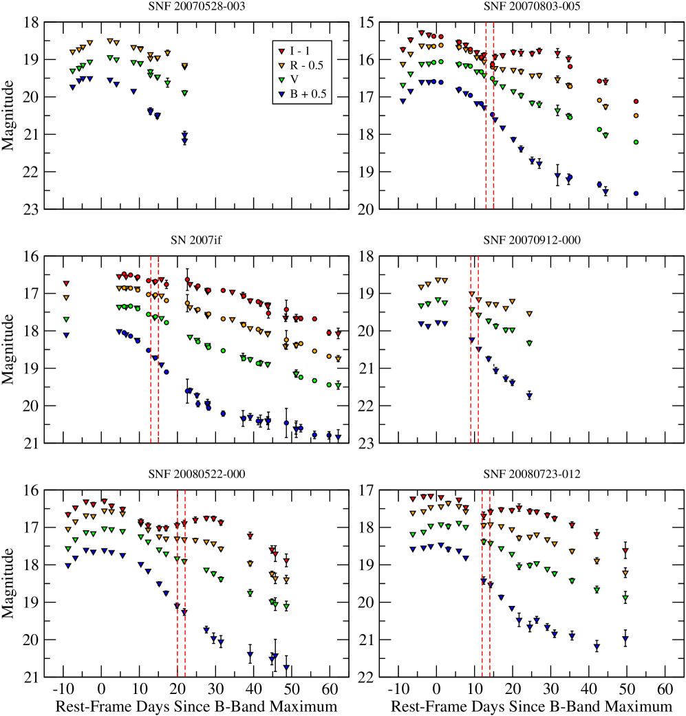
Figure 1.— Rest-frame Bessell $BVRI$ light curves from ANDICAM+SNIFS. Inverted triangles: Rest-frame Bessell $BVRI$ magnitudes synthesized from SNIFS flux-calibrated spectroscopy. Circles: ANDICAM $BVRI$, $K$-corrected to the respective rest-frame Bessell filters. Vertical dotted red lines mark the light curve phase range corresponding to the break in $v$(Si II)discussed in §3.3.

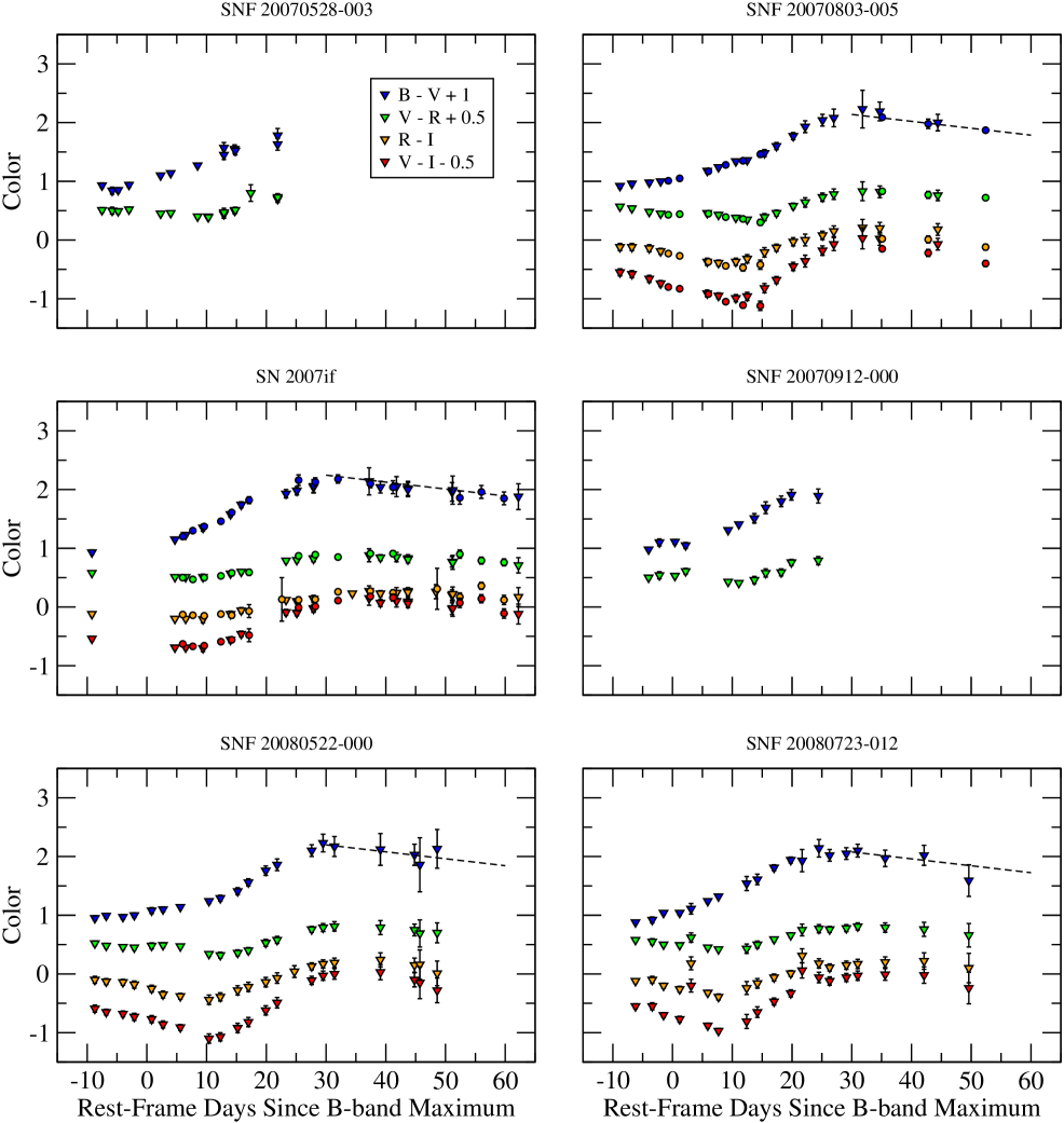
Figure 2.— Rest-frame Bessell color evolution from ANDICAM (circles) and SNIFS spectrophotometry (inverted triangles). Dotted lines indicate fits to the Lira relation with a floating excess.

2.5. Spectra

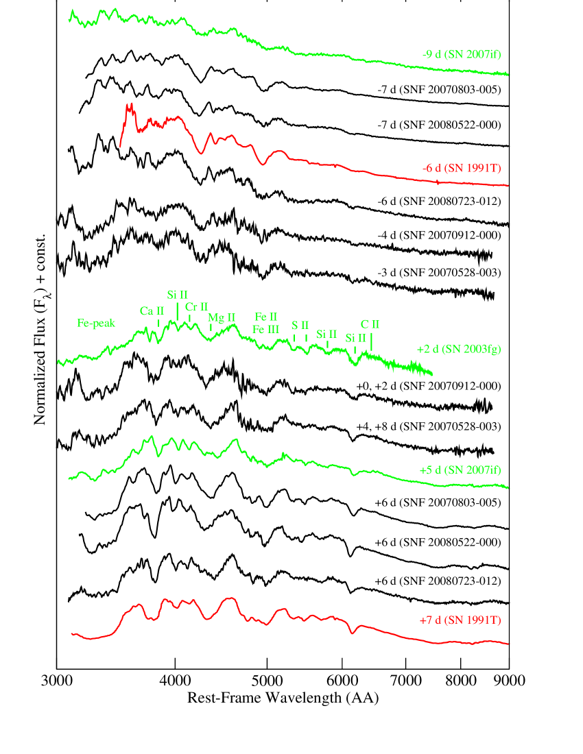
Figure 3.— Selected spectra near maximum light of SNfactory candidate super-Chandra SNe Ia (black), with spectra of SN 1991T (red) at $-6$ d (Mazzali et al., 1995) and at $+7$ d (Filippenko et al., 1992), and the candidate super-Chandra events SN 2003fg (Howell et al., 2006, green) and SN 2007if (Scalzo et al., 2010, green) for comparison. Spectra have been smoothed with a 15-point (width 2000 km s^-1) Savitzsky-Golay filter for presentation purposes. Consecutive post-maximum spectra of the $z\sim 0.12$ SNe SNF 20070528-003 and SNF 20070912-000 have been co-added to improve signal-to-noise. Common features identified with SYNAPPS (Thomas et al., 2011) are marked.

Figure 3 presents the subset of spectra that were taken near maximum light for the six SNfactory SNe Ia, including SN 2007if. Before maximum light, the spectra show weak Si II, S II, and Ca II absorption plus strong Fe II and Fe III absorption, in accordance with our selection criteria. SN 1991T and the prototype candidate super-Chandra SN Ia 2003fg are shown for comparison. After maximum light, some features noted in SN 2003fg and SN 2007if appear, including the iron-peak blend near 4500 Å, the sharp notch near 4130 Å identified as Cr II in Scalzo et al. (2010) (or tentatively as C II $\lambda 4237$ in Howell et al., 2006) and the blended lines near 3300 Å identified as Cr II and Co II in Scalzo et al. (2010). (The 4130 Å feature is not clearly present in the $z=0.123$ candidate SNF 20070912-000, although this may be due to the lower S/N of the spectrum.) Taubenberger et al. (2011) note that a similar feature in SN 2009dc strengthens with time rather than fading, as one would expect for Cr II rather than C II.

SN 2007if also shows a weak C II $\lambda 6580$ line in the post-maximum spectra, which Scalzo et al. (2010) interpreted as a signature of unburned material from the explosion. While this line is not detected unambiguously in the other SNe, the unusually shallow slope of the red wing of Si II $\lambda 6355$ e.g. in SNF 20070528-003 and SNF 20080723-012 may be a sign that C II is present in these SNe (Thomas et al., 2011). The spectral properties of the full dataset are analyzed in §3.3.

3. Analysis

The analysis (this section), modeling (§4) and interpretation (§5) for our sample parallels that made for SN 2007if in Scalzo et al. (2010), with improvements described below. We include a re-analysis of our observations of SN 2007if in this paper using the improved techniques, for a more direct comparison with the other SNe presented in this paper.

3.1. Maximum-Light Behavior, Colors and Extinction

Table 3Derived quantities from SALT2 fits to light curves

SN Name	MJD($B_{\mathrm{max}}$)	$M_{V}$	$x_{1}$	$c$	$\chi^{2}/\nu$	$\Delta m_{15}(B)$	$(B-V)_{\mathrm{max}}$	$B_{\mathrm{max}}-V_{\mathrm{max}}$	$\Delta mu$
SNF 20070528-003	$54258.7$	$-19.71\pm 0.02$	$1.08\pm 0.20$	$0.02\pm 0.03$	1.82	$0.84\pm 0.05$	$0.01\pm 0.04$	$0.03\pm 0.04$	$-0.48$
SNF 20070803-005	$54327.6$	$-19.59\pm 0.04$	$1.04\pm 0.09$	$0.01\pm 0.03$	0.74	$0.85\pm 0.05$	$0.00\pm 0.04$	$0.02\pm 0.04$	$-0.28$
SN 2007if	$54346.8$	$-20.38\pm 0.02$	$1.41\pm 0.13$	$0.12\pm 0.03$	3.48	$0.79\pm 0.06$	$0.12\pm 0.05$	$0.14\pm 0.04$	$-1.34$
SNF 20070912-000	$54363.0$	$-19.69\pm 0.02$	$-0.03\pm 0.19$	$0.04\pm 0.03$	1.41	$1.08\pm 0.04$	$0.05\pm 0.02$	$0.06\pm 0.02$	$-0.52$
SNF 20080522-000	$54621.4$	$-19.59\pm 0.03$	$1.18\pm 0.13$	$-0.01\pm 0.03$	0.43	$0.83\pm 0.06$	$-0.02\pm 0.04$	$0.00\pm 0.04$	$-0.17$
SNF 20080723-012	$54680.9$	$-19.71\pm 0.02$	$0.53\pm 0.12$	$0.04\pm 0.03$	2.61	$0.93\pm 0.04$	$0.03\pm 0.03$	$0.05\pm 0.03$	$-0.59$

As discussed in Scalzo et al. (2010), SN 2007if shows no distinct second maximum. While Figure 1 does show second maxima for our other SNe, its prominence is suppressed relative to normal SNe Ia. In SNF 20070803-005 and SNF 20080723-012, the peak-to-trough difference in a quintic polynomial fit to the data from day +7 to day +42 is only 0.11 mag, vs. 0.23 mag for SNF 20080522-000 and 0.35 mag for the SALT2 model with $x1=1$, $c=0$. Kasen (2006) noted three physical effects which could reduce the contrast of the $I$-band second maximum: low ${}^{56}\mathrm{Ni}$ mass, efficient mixing of ${}^{56}\mathrm{Ni}$ into the outer layers of ejecta, and greater absorption in the Ca II NIR triplet line source function. Since our SNe are all overluminous with broad light curves, Arnett’s rule gives a high nickel mass, as we find in the next section. The $I$-band first maximum is roughly concurrent with $B$-band maximum for our SNe, rather than being significantly delayed (see figure 14 of Kasen, 2006), so it seems unlikely that emission in the Ca II NIR triplet is contributing significantly. The most likely interpretation, especially given the prominence of Fe-peak lines in early spectra of our SNe, is that ${}^{56}\mathrm{Ni}$ is well-mixed into the outer layers.

Following practice from Scalzo et al. (2010), we use the updated version (v2.2) of the SALT2 light curve fitter (Guy et al., 2010) to interpolate the magnitudes and colors of each SN around maximum light, and to establish a date of $B$-band maximum with respect to which we can measure light-curve phase. While we use SALT2 here as a convenient functional form for describing the shape of the light curves near maximum light, and to extract the usual parameters describing the light curve shape, we do not expect the SALT2 model, trained on normal SNe Ia, to give robust predictions for these peculiar SNe Ia outside the phase and wavelength coverage for each SN. To minimize the impact of details of the SALT2 spectral model on the outcome, we use SALT2 in the rest frame, include SALT2 light curve model errors in the fitting, and we fit $BVR$ bands only; $I$-band is excluded from the fit. The quantities derived from the SALT2 light curve fits are shown in Table 3. A cross-check in which cubic polynomials were fitted to each band produces peak magnitudes and dates of maximum in each band consistent with the SALT2 answers, within the errors, for all of the new SNe; we adopt the SALT2 values as our fiducial values for direct comparison with other work.

We estimate the host reddening of the SNe in two separate ways. First, we fit the $B-V$ color behavior of each SN to the Lira relation (Phillips et al., 1999; Folatelli et al., 2009) for those SNe for which we have appropriate light curve phase coverage. The Lira relation is believed explicitly not to hold for SN 2007if and the candidate super-Chandra SN Ia 2009dc (Yamanaka et al., 2009; Taubenberger et al., 2011), but its value may nevertheless be useful in studying the relative intrinsic color of these SNe. Additionally, we search for New A absorption at the redshift of the host galaxy for each SN. We perform a $\chi^{2}$ fit to the New A line profile, modeled as two separate Gaussian lines with full width at half maximum equal to the SNIFS instrumental resolution of 6 Å, to all SNIFS spectra of each SN, as for SN 2007if in Scalzo et al. (2010). In the fit, the equivalent width $EW$(Na I D) of the New A line is constrained to be non-negative. We convert these to estimates of $E(B-V)_{\mathrm{host}}$ using both the shallow-slope (0.16 Å^-1) and steep-slope (0.51 Å^-1) relations from Turatto, Benetti & Cappellaro (2002) (“TBC”). While the precision of these relations has been called into question when used on their own (e.g. Poznanski et al., 2011), we believe that examining such estimates together with the Lira relation and fitted colors from the light curve can provide helpful constraints on the importance of host reddening. The best-fit Lira excesses, values of $EW$(Na I D), and derived constraints on the host galaxy reddening are listed in Table 4.

We detect weak New A absorption in SNF 20070803-005 and SNF 20080522-000. Neither of these SNe appear to have very red colors according to the SALT2 fits, and we believe it to be unlikely that either are heavily extinguished, so for purposes of extinction corrections to occur later in our analysis, we use reddening estimates from the shallow-slope TBC relation, together with a CCM dust law with $R_{V}=3.1$ (Cardelli et al., 1988). When applied to Milky Way New A absorption in our spectra, the shallow-slope TBC relation produces $E(B-V)$ estimates consistent with Schlegel et al. (1998). SNF 20070912-000 shows a marginal ($<2\sigma$) detection, though the spectra are noisy and the limits are not strong. We detect no New A absorption in the other SNe.

Table 4Host galaxy reddening estimates from the Lira relation and $EW$(Na I D) fits

	Na I D	Shallow	Steep	Lira
SN Name	EW (Å)	TBC	TBC	Relation
SNF 20070528-003	$0.00^{+0.32}_{-0.00}$	$0.00^{+0.05}_{-0.00}$	$0.00^{+0.12}_{-0.00}$	$\cdots$
SNF 20070803-005	$0.19^{+0.05}_{-0.06}$	$0.02^{+0.01}_{-0.01}$	$0.06^{+0.03}_{-0.03}$	$0.06\pm 0.06$
SN 2007if	$0.00^{+0.12}_{-0.00}$	$0.00^{+0.01}_{-0.00}$	$0.00^{+0.02}_{-0.00}$	$0.13\pm 0.07$
SNF 20070912-000	$0.32^{+0.44}_{-0.18}$	$0.04^{+0.07}_{-0.03}$	$0.12^{+0.22}_{-0.09}$	$\cdots$
SNF 20080522-000	$0.29^{+0.08}_{-0.08}$	$0.04^{+0.01}_{-0.01}$	$0.11^{+0.04}_{-0.04}$	$0.13\pm 0.12$
SNF 20080723-012	$0.00^{+0.19}_{-0.00}$	$0.00^{+0.02}_{-0.00}$	$0.00^{+0.06}_{-0.00}$	$0.00\pm 0.10$

Based on the very strong limit on New A absorption from the host galaxy, Scalzo et al. (2010) inferred that the large Lira excess of SN 2007if was not due to host galaxy extinction. Those SNe observed at sufficiently late phases show measured Lira excesses consistent with zero, additional evidence that host galaxy dust extinction is minimal for these SNe if the Lira relation holds.

Allowing for varying amounts of extinction associated with the Lira excess or New A absorption, each of the new SNe have maximum-light $(B-V)$ colors consistent with zero. While most of our SNe have well-sampled light curves around maximum light and hence have well-measured maximum-light colors, SN 2007if has a gap between $-9$ days and $+5$ days with respect to $B$-band maximum (phases fixed by the SALT2 fit). The light curve fit of (Scalzo et al., 2010), using SALT2 v2.0 and a spectrophotometric reduction using a previous version of the SNIFS pipeline, suggests a red color $B-V=0.16\pm 0.06$. The more recent reduction fit with SALT2 v2.2 gives $B-V=0.12\pm 0.06$. However, the directly measured $B-V$ color of SN 2007if at $-9$ days ($-0.07\pm 0.04$) and at $+5$ days ($0.15\pm 0.02$) are each consistent within the errors with the mean values at those epochs for our other five SNe. The systematic error on the maximum-light color of SN 2007if, at least 0.04 mag, may therefore be too large for it to be considered significantly redder at maximum than its counterparts.

3.2. Bolometric Light Curve and ${}^{56}\mathrm{Ni}$ Synthesis

As input to our further analysis to calculate ${}^{56}\mathrm{Ni}$ masses and total ejected masses for our sample of SNe, we calculate quasi-bolometric UVOIR light curves from the photometry. To derive bolometric fluxes from SNIFS spectrophotometry, we first deredden the spectra to account for Milky Way dust reddening (Schlegel et al., 1998), then deredden by an additional factor corresponding to a possible value of the host galaxy reddening, creating a suite of spectra covering the range $0.00<E(B-V)_{\mathrm{host}}<0.40$ in 0.01 mag increments. We then integrate the dereddened, deredshifted, flux-calibrated spectra over all rest-frame wavelengths from 3200–9000 Å. For each quasi-simultaneous set of ANDICAM $BVRI$ observations and each possible value of $E(B-V)_{\mathrm{host}}$, we multiply the dereddened, deredshifted SNIFS spectrum nearest in time by a cubic polynomial, fitted so that the synthetic photometry from the resulting spectrum matches, in a least-squares sense, the ANDICAM imaging photometry in each band. We then integrate this “warped” spectrum to produce the bolometric flux from ANDICAM. This procedure creates a set of bolometric light curves with different host galaxy reddening values which we can use in our later analysis (see §4).

SNF 20070528-003 and SNF 20070912-000 are at a higher redshift than our other SNe, such that SNIFS covers only the rest-frame wavelength range 3000–8500 Å, so we integrate their spectra in this range instead. We expect minimal systematic error from the mismatch, since the phase coverage for these two SNe is such that only the bolometric flux near maximum light, when the SNe are still relatively blue, is useful for the modeling described in §4.

To account for the reprocessing of optical flux into the near-infrared (NIR) by iron-peak elements over the evolution of the light curve, we must apply a NIR correction to the integrated SNIFS fluxes. No NIR data were taken for any of the SNe except SN 2007if; in general they were too faint to observe effectively with the NIR channel of ANDICAM. Since these are peculiar SNe, any correction for the NIR flux necessarily involves an extrapolation. Since the $I$-band second maximum has low contrast for all the SNe in our sample, the $JHK$ behavior should be similar for these SNe to the extent that $I$ and $JHK$ are related (e.g. as in Kasen, 2006). With these caveats, we therefore use the NIR corrections for SN 2007if derived in Scalzo et al. (2010) for all of our SNe, with the time axis stretched according to the stretch factor derived from the SALT2 $x_{1}$ (Guy et al., 2007) to account for the different timescales for the development of line blanketing in these SNe. Our modeling requires knowledge of the bolometric flux only near maximum light (to constrain the ${}^{56}\mathrm{Ni}$ mass) and more than 40 days after maximum light (to constrain the total ejected mass). The NIR correction is at a minimum near maximum light ($\sim 5\%$), and at a maximum near phase $+40$ days ($\sim 25\%$), so it should not evolve quickly at these times and our results should not be strongly affected. We assign a systematic error of $\pm 5\%$ of the total bolometric flux (or about $\pm 30\%$ of the NIR flux itself near $+40$ d) to this correction.

To estimate ${}^{56}\mathrm{Ni}$ masses, we also need a measurement of the bolometric rise time $t_{\mathrm{rise,bol}}$. We establish the time of bolometric maximum light $t_{\mathrm{max,bol}}$ by fitting a cubic polynomial to the bolometric fluxes in the phase range $-10~{}\mathrm{d}<t<+20~{}\mathrm{d}$. We then calculate the final bolometric rise time $t_{\mathrm{rise,bol}}$ via

$$t_{\mathrm{rise,bol}}=t_{\mathrm{rise,}B}-t_{\mathrm{max,}B}+t_{\mathrm{max,bol}}.$$ (1)

We find $t_{\mathrm{max,bol}}$ to occur about 1 day earlier than $t_{\mathrm{max,}B}$ for the SNe in our sample. We have a strong constraint on the time of explosion only for SN 2007if (Scalzo et al., 2010), for which this procedure results in a bolometric rise time of 23 days. We have utilized the discovery data from our search along with our spectrophotometry to constrain the rise times of the new SNe presented here. For these we find $t_{rise,B}=21.2\pm 1.9$ days, and so use $t_{rise,bol}=20\pm 2$ days in our models. Our value is very similar to the value of $t_{\mathrm{rise,}B}=21\pm 2$ days given by the sample of 1991T-like SNe Ia in Ganeshalingam et al. (2011). This approach leads to more conservative uncertainties than the single-stretch correction of Conley et al. (2006); Figure 6 of Ganeshalingam et al. (2011) suggests that the relation between rise time and decline rate $\Delta m_{15}$ (or stretch $s$) may break down at the high-stretch end.

We calculate the ${}^{56}\mathrm{Ni}$ mass, $M_{\mathrm{Ni}}$, for the six SNe by relating the maximum-light bolometric luminosity $L_{\mathrm{bol}}$ to the luminosity from radioactive decay $L_{\mathrm{rad}}$ (Arnett, 1982):

$$\alpha^{-1}L_{\mathrm{bol}}\ = \ L_{\mathrm{rad}}$$ (2)

$$= \ N_{{}^{56}\mathrm{Ni}}\lambda_{{}^{56}\mathrm{Ni}}Q_{{{}^{56}\mathrm{Ni}},\gamma}\,e^{-\lambda_{{}^{56}\mathrm{Ni}}t}$$

$$+ \ N_{{}^{56}\mathrm{Ni}}\lambda_{{}^{56}\mathrm{Ni}}\frac{\lambda_{{}^{56}\mathrm{Co}}}{\lambda_{{}^{56}\mathrm{Ni}}-\lambda_{{}^{56}\mathrm{Co}}}\left(Q_{{{}^{56}\mathrm{Co}},e^{+}}+Q_{{{}^{56}\mathrm{Co}},\gamma}\right)$$

$$\ \ \ \ \times\left(e^{-\lambda_{{}^{56}\mathrm{Co}}t}-e^{-\lambda_{{}^{56}\mathrm{Ni}}t}\right),$$

where $t$ ($=t_{\mathrm{rise,bol}}$ in this case) is the time since explosion, $N_{{}^{56}\mathrm{Ni}}=M_{{}^{56}\mathrm{Ni}}/(56~{}\mathrm{AMU})$ is the number of ${}^{56}\mathrm{Ni}$ atoms produced in the explosion, $\lambda_{{}^{56}\mathrm{Ni}}$ and $\lambda_{{}^{56}\mathrm{Co}}$ are the decay constants for ${}^{56}\mathrm{Ni}$ and ${}^{56}\mathrm{Co}$ ($e$-folding lifetimes 8.8 days and 111.1 days) respectively, and $Q_{{{}^{56}\mathrm{Ni}},\gamma}$, $Q_{{{}^{56}\mathrm{Co}},\gamma}$ and $Q_{{{}^{56}\mathrm{Co}},e^{+}}$ are the energies released in the different stages of the decay chain (Nadyozhin, 1994). The dimensionless number $\alpha$ is a correction factor accounting for the diffusion time delay of gamma-ray energy through the ejecta, typically ranging between 0.8 and 1.6 for reasonable explosion models (see e.g., Table 2 of Höflich & Khohklov, 1996, where it is called $Q$). A nominal value of $\alpha=1.2$ is often used in the literature (e.g. Nugent et al., 1995; Branch & Khokhlov, 1995; Howell et al., 2006, 2009). The tamped detonation models of Khokhlov et al. (1993) and Höflich & Khohklov (1996), on which we will base our modeling later in the paper, have slightly higher values closer to $\alpha=1.3$. We therefore adopt a fiducial value of $\alpha=1.3$ for our simple estimate here.

Table 5${}^{56}\mathrm{Ni}$ mass reconstruction for the SNfactory SNe

SN Name	$L_{\mathrm{bol}}$ ($10^{43}$ erg s-1)	$t_{\mathrm{rise,bol}}$ (d)	$M_{\mathrm{Ni}}~{}(M_{\odot})$
SNF 20070528-003	$1.87\pm 0.06$	$20\pm 2$	$0.78\pm 0.11$
SNF 20070803-005	$1.62\pm 0.05$	$20\pm 2$	$0.69\pm 0.07$
SN 2007if	$2.93\pm 0.22$	$23\pm 2$	$1.38\pm 0.09$
SNF 20070912-000	$1.86\pm 0.06$	$20\pm 2$	$0.77\pm 0.10$
SNF 20080522-000	$1.70\pm 0.06$	$20\pm 2$	$0.74\pm 0.08$
SNF 20080723-012	$1.82\pm 0.07$	$20\pm 2$	$0.76\pm 0.10$

The resulting ${}^{56}\mathrm{Ni}$ mass estimates are shown in Table 5. The new SNe have $M_{\mathrm{Ni}}$ in the range 0.7–0.8 $M_{\odot}$, at the high end of what might be expected for Chandrasekhar-mass explosions; the well-known W7 deflagration model (Nomoto et al., 1984) produced 0.6 $M_{\odot}$ of ${}^{56}\mathrm{Ni}$, while some delayed detonation models can produce up to 0.8 $M_{\odot}$ (e.g., the N21 model of Höflich & Khohklov, 1996).

3.3. Spectral Features and Velocity Evolution

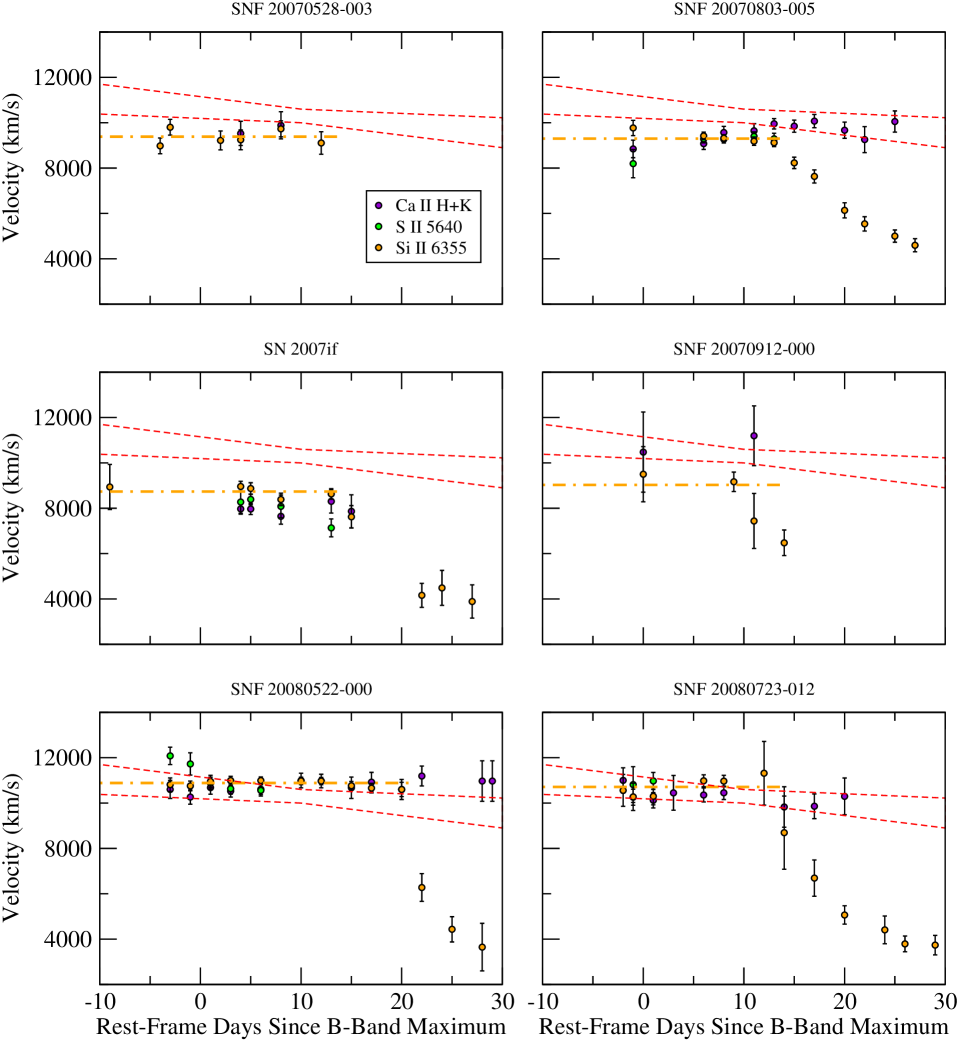
Figure 4.— Time evolution of the velocities of various intermediate-mass-element absorption minima from the super-Chandra candidate sample: Si II $\lambda 6355$, S II $\lambda 5640$, and Ca II H+K. The thick dash-dot line shows a $\chi^{2}$ fit to a constant for all $v$(Si II) data before the end of the plateau phase for each SN. The thin dashed lines show the 1-sigma range of behavior for the LVG subclass of Benetti et al. (2005).

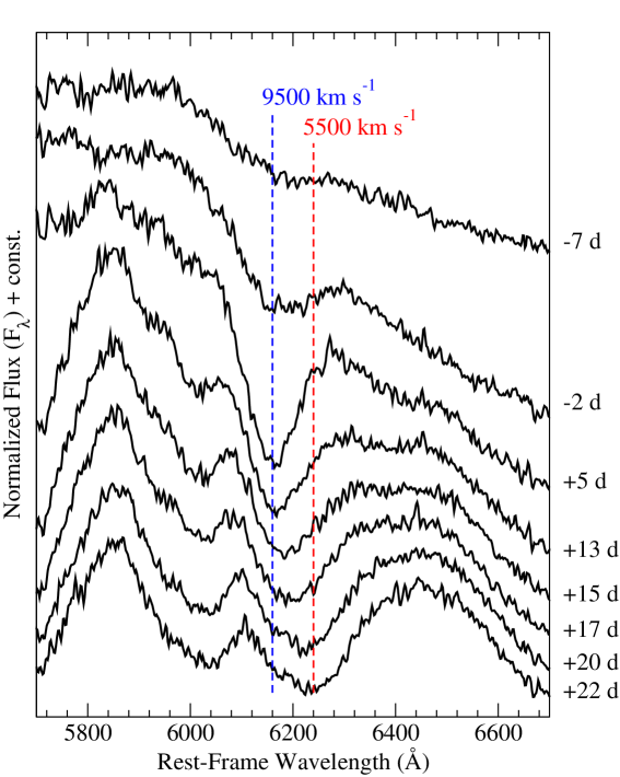
Figure 5.— Detailed evolution of SNF 20070803-005 spectra around the Si II $\lambda 6355$ feature.

The time evolution of the position of the Si II $\lambda 6355$ absorption minimum, showing the recession of the photosphere through the ejecta, is shown in Figure 4. The measurements of the absorption minimum were made as follows: bins in each spectrum immediately to the right and left of the line feature were used to fit a linear pseudocontinuum, $F_{\lambda,\mathrm{cont}}=a+b\lambda$. This fitted pseudocontinuum was divided into each bin of the spectrum in the region of the line. The resulting spectrum was smoothed with a third-order Savitzsky-Golay filter and the minimum was recorded as the bin with the lowest signal. The error bars on the procedure were determined through a bootstrap Monte Carlo: In the first stage, values of $a$ and $b$ representing possible pseudocontinua $F_{\lambda,\mathrm{cont}}$ were sampled using the covariance matrix of the pseudocontinuum fit; for each candidate pseudocontinuum, fluctuations typical of the measured errors on each spectral bin were added to the smoothed spectrum, and the results were smoothed and the minimum measured again. We have verified that the Savitzsky-Golay filter preserves the line minimum, so that smoothing a spectrum twice introduces negligible systematic error. The final velocity values and their errors were measured as the mean and standard deviation of the distribution of absorption minimum velocities thus generated. While this method has slightly less statistical power than a fit to the entire line profile as in Scalzo et al. (2010), we believe it is more robust to possible bias from line profiles with unusual shapes, and provides more realistic error bars for the line minimum.

Table 6Velocity gradient characteristics

SN Name	$v_{\mathrm{pl}}$		$\dot{v}$		$t_{\mathrm{pl,0}}$	$\Delta t_{\mathrm{pl}}$	$\chi^{2}_{\nu}$
SNF 20070528-003	9371 $\pm$	171	$-6$ $\pm$	29	$-4$	$16$	0.85
SNF 20070803-005	9695 $\pm$	81	$46$ $\pm$	23	$-1$	$14$	1.00
SN 2007if	8963 $\pm$	248	$31$ $\pm$	29	$-9$	$21$	0.76
SNF 20070912-000	9201 $\pm$	403	$\cdots$		$\cdots$	$\cdots$	$\cdots$
SNF 20080522-000	10936 $\pm$	107	$5$ $\pm$	10	$-4$	$16$	0.41
SNF 20080723-012	10391 $\pm$	291	$-72$ $\pm$	47	$-2$	$10$	0.72

We found that for lines with equivalent widths less than 15 Å, the absorption minima had unreasonably large uncertainties and/or showed large systematic deviations from the trend described by stronger measurements. When measuring these absorption minima, we are probably simply measuring uncertainty in the pseudocontinuum. Blondin et al. (2011) saw similar effects when measuring velocities of very weak absorption minima, to the extent that the Si II $\lambda 6355$ velocity would even be seen to increase with time. We therefore reject measurements of such weak absorption features.

Our candidate super-Chandra SNe Ia share a slow evolution of the Si II velocity, consistent within the errors with being constant in time for each SN from the earliest phases for which measurements are available. Table 6 shows the fitted constant velocities and the chi-square per degree of freedom, $\chi^{2}_{\nu}$, for a fit to a constant. For comparison with earlier work, the velocity gradient $\dot{v}=-dv/dt$ calculated as the slope of the best-fit linear trend of the measurements before day $+14$, is also listed, along with the formal error from the fit. All of our SNe would be classified as Benetti LVG (Benetti et al., 2005) based on their velocity gradients. While the slope of the straight-line fit to the absorption velocities for SNF 20070803-005 seems to differ from zero at the $2\sigma$ level (formal errors), the reduced chi-square for this fit is extremely small ($\chi^{2}_{\nu}=0.006$) and we conclude that the evolution cannot be reliably distinguished from a constant ($\chi^{2}_{\nu}=1.00$). Similarly, the best-fit line to the absorption velocities for SNF 20080723-012 has a positive slope at $1.5\sigma$ ($\dot{v}=72\pm 47~{}\mathrm{km~{}s}^{-1}$ day^-1), but once again, a constant is a good fit to the data ($\chi^{2}_{\nu}=0.72$).

The slow Si II absorption velocity evolution usually lasts until about two weeks after maximum light, after which a break in the behavior occurs and a pronounced decline begins, at a rate of $\sim 500~{}\mathrm{km~{}s}^{-1}~{}\mathrm{day}^{-1}$. At this point, developing Fe II lines have probably blended with Si II and made the velocity measurements unreliable (see, e.g. Phillips et al., 1992). The transition occurs concurrently with the onset of the second maximum in the $I$-band light curve, which may be attributed to light reprocessed from bluer wavelengths by the recombination of Fe III to Fe II as the ejecta expand and cool (Kasen, 2006). Figure 5 shows the evolution of the Si II $\lambda 6355$ line profile for SNF 20070803-005 near the transition. The line profile after the break shows a portion of the Si II line near the plateau velocity, suggesting that the material responsible for the plateau has thinned but is not yet transparent. We mark the phases of the last $v$(Si II) measurement visually consistent with the plateau velocity, and the first measurement inconsistent with it, by vertical dashed lines in Figure 1 to show their correspondence with the $I$-band second maximum.

In four of the six SNe, the plateau velocity is low ($\sim~{}9000$ km s^-1), inconsistent with the normal range of behavior of the LVG subclass of Benetti et al. (2005). The remaining two SNe, SNF 20080522-000 and SNF 20080723-012, have higher plateau velocities ($\sim 11000$ km s^-1), falling roughly into the range of LVG behavior, although their velocity gradients are still flatter than any remarked upon in that work. Due to the lower S/N of our spectra of SNF 20070912-000 and the weakness of the Si II $\lambda 6355$ absorption feature, only two measurements of the line velocity before the break, each around 9000 km/s with large errors, were extracted; we can at most say that the observed velocity gradient in this SN is consistent with that of the other SNe in our sample.

Figure 4 also shows the line minimum velocities of Ca II H+K and S II $\lambda\lambda 5456,5640$. Although, as expected, Ca II H+K stays optically thick longer than Si II $\lambda 6355$, its velocities at early times are consistent with the observed plateau behavior shown by Si II. The S II lines are weak, but when their absorption minima can be reliably measured, they do not show dramatically higher or lower velocities than the other lines. This supports the interpretation that all of these lines are formed in the same thin, dense layer of ejecta.

4. Constraints on Total Mass and Density Structure

The modeling procedure we use here represents a refined version of that used in Scalzo et al. (2010), which we compare and contrast with the similar approach of Stritzinger et al. (2006) in §4.1 for the special case of a simple equivalent exponential density profile. We then describe our extensions to the method, including modeling of density profiles with shells (§4.2), priors on the central density (§4.3), and calculation of the ${}^{56}\mathrm{Ni}$ form factor $q$ (§4.4). We then present our final modeling results in §4.5.

4.1. SN Ia Ejected Mass Measurements Using the Equivalent Exponential Density Formalism

The ejecta density structure of SNe Ia is frequently modeled as an exponential $\rho(v)\propto\exp(-v/v_{e})$, where the ejecta are in homologous expansion at velocity $v=(r-r_{\mathrm{initial}})/t$ since the explosion at time $t=0$, and $v_{e}$ is a characteristic velocity scale. Many hydrodynamic models of SN Ia explosions, including the well-known W7 model (Nomoto et al., 1984), have density profiles which are very close to exponential.

Jeffery (1999) made semianalytic calculations of the time evolution of the gamma-ray energy deposition in an exponential model SN Ia, with reference to its bolometric light curve. By about 60 days after explosion, virtually all of the ${}^{56}\mathrm{Ni}$ has decayed and the dominant energy source is the decay of ${}^{56}\mathrm{Co}$ (which in turn was produced by ${}^{56}\mathrm{Ni}$ decay at earlier times). The optical depth to Compton scattering of ${}^{56}\mathrm{Co}$ gamma rays behaves as $\tau_{\gamma}=(t/t_{0})^{-2}$ with $\tau_{\gamma}=1$ at some fiducial time $t_{0}$. The value of $t_{0}$ can be extracted by fitting the bolometric light curve for $t>60$ d to a modified version of Equation 2, in which $\alpha=1$ (rather than its maximum-light value from Arnett’s rule) and the term corresponding to ${}^{56}\mathrm{Co}$ gamma rays is multiplied by a factor $1-\exp(-\tau_{\gamma})$. The total mass of the ejecta can then be expressed as

$$M_{\mathrm{WD}}=\frac{8\pi}{\kappa_{\gamma}q}(v_{e}t_{0})^{2}.$$ (3)

Here, $\kappa_{\gamma}$ is the Compton scattering opacity for ${}^{56}\mathrm{Co}$ gamma rays, and $q$ is a form factor describing the distribution of the ${}^{56}\mathrm{Co}$ in the ejecta, which follows the original distribution of ${}^{56}\mathrm{Ni}$ in the explosion. The value of $\kappa_{\gamma}$ is expected to lie in the range 0.025–0.033 cm^-2 g (Swartz et al., 1995), with the low end (0.025) corresponding to the optically thin regime. The value of $q$ can be readily calculated given an assumed distribution of ${}^{56}\mathrm{Ni}$ (see §4.4 below).

Stritzinger et al. (2006) used this method to measure progenitor masses for a sample of well-observed SNe Ia with $UBVRI$ light curve coverage. They constructed “quasi-bolometric” light curves according to the procedure of Contardo, Leibundgut & Vacca (2000), by converting the observed $UBVRI$ magnitudes to monochromatic fluxes at the central wavelengths of their respective filters, then summing them, using corrections for lost flux between filters derived from spectroscopy of SN 1992A. They then applied the semianalytic approach of Jeffery (1999) to fit for the gamma-ray escape fraction, and hence the ejected mass of the SN Ia progenitor.

Our own work improves on previous use of this method in two important ways. First, Stritzinger et al. (2006) made no attempt to correct for the NIR contribution to the bolometric flux, simply asserting that it is small during the epochs of interest. In Scalzo et al. (2010) we found that for SN 2007if the NIR contribution was indeed small ($\sim 5\%$) near maximum light, but was greater than 25% at 40 days after maximum light, and our estimate for its value at 100 days after maximum light is still around 10%. Therefore, at least for SNe Ia like the ones we study here, the method of Stritzinger et al. (2006) underestimates the fraction of trapped ${}^{56}\mathrm{Co}$ gamma-rays for a given initial ${}^{56}\mathrm{Ni}$ mass, and hence the ejected mass, as a result of neglecting NIR flux.

Second, our fitting procedure includes covariances between different inputs to the prediction for the bolometric light curve, constrained by a set of Bayesian priors motivated by explosion physics. Specifically, covariances between $q$, $v_{e}$, and $\alpha$ may influence the interpretation of the fitted value of $t_{0}$. Stritzinger et al. (2006) simply fixed the ${}^{56}\mathrm{Ni}$ mass from Arnett’s rule, and then fit for $t_{0}$. Similarly, they assume $q=1/3$, $v_{e}=3000$ km s^-1, and $\alpha=1$ for all of their SNe, with no covariance between any of these parameters. Because models with more ${}^{56}\mathrm{Ni}$ need less gamma-ray trapping to produce the same bolometric luminosity at a given time, there is a large fitting covariance between the ${}^{56}\mathrm{Ni}$ mass and $t_{0}$, mentioned in Scalzo et al. (2010). The value of $\alpha$ is model-dependent, and not a fundamental physical quantity, but as noted in §3.2 above, $\alpha=1.2$ ($\pm 0.1$) is also a common choice when no other prior is available from explosion models. Since $\alpha$ affects the nickel mass, a smaller assumed value of $\alpha$ results in a larger ${}^{56}\mathrm{Ni}$ mass, but a smaller ejected mass, as interpreted from a given bolometric light curve. In a self-consistent choice of parameters, $v_{e}$ and $q$ will each depend in part on the mass of ${}^{56}\mathrm{Ni}$ and therefore on $\alpha$.

The value of $v_{e}$ is difficult to measure directly, since observed velocities of absorption line minima may depend on temperature as much as density. Since $v_{e}$ appears squared in Equation 3, its contribution to the error budget on $M_{\mathrm{WD}}$ is potentially quite large if treated as an independent input. However, its value can be constrained within a range of $\pm 300$ km s^-1 by requiring energy conservation. Following practice in the literature (Howell et al., 2006; Maeda & Iwamoto, 2009), we calculate the kinetic energy $E_{K}$ as the difference between the energy $E_{N}$ released in nuclear burning and the gravitational binding energy $E_{G}$, and then set $v_{e}=(E_{K}/6M_{\mathrm{WD}})^{1/2}$.

Calculating the energy budget of a SN Ia requires us to assume a composition. Our model considers four components to the ejecta:

• ${}^{56}\mathrm{Ni}$, which contributes to the luminosity, $E_{N}$, and $E_{G}$;

• Stable Fe-peak elements (“Fe”), which contribute to $E_{N}$ and $E_{G}$;

• Intermediate-mass elements such as Mg, Si and S (“Si”), which contribute to $E_{N}$ and $E_{G}$;

• Unburned carbon and oxygen (“C/O”), which contribute only to $E_{G}$.

The input parameters, which we vary using a Metropolis-Hastings Monte Carlo Markov chain, are the white dwarf mass $M_{\mathrm{WD}}$, the central density $\rho_{c}$ (needed in the calculation of $E_{G}$), the parameter $\alpha$ from Arnett’s rule, the bolometric rise time $t_{\mathrm{rise,bol}}$, and the fractions $f_{\mathrm{Ni}}$, $f_{\mathrm{Fe}}$, and $f_{\mathrm{Si}}$ of ${}^{56}\mathrm{Ni}$, stable Fe, and intermediate-mass elements within $M_{\mathrm{WD}}$. We fix the fraction of unburned carbon and oxygen $f_{\mathrm{CO}}=1-f_{\mathrm{Fe}}-f_{\mathrm{Ni}}-f_{\mathrm{Si}}$. We use the prescription of Maeda & Iwamoto (2009) to determine $E_{N}$:

$$E_{N}=\left[1.74f_{\mathrm{Fe}}+1.56f_{\mathrm{Ni}}+1.24f_{\mathrm{Si}}\right]\left(\frac{M_{\mathrm{WD}}}{M_{\odot}}\right)\times 10^{51}\mathrm{erg}.$$ (4)

We use the binding energy formulae of Yoon & Langer (2005) for $E_{G}=E_{G}(M_{\mathrm{WD}},\rho_{c})$, where $\rho_{c}$ is the white dwarf central density. These ingredients determine $v_{e}$. We apply Gaussian priors $\alpha=1.3\pm 0.1$ (as for SN 2007if; Scalzo et al., 2010) and $t_{\mathrm{rise,bol}}=20\pm 2$ days, and on $E(B-V)_{\mathrm{host}}$ according to the “shallow TBC” values in Table 4. We adopt $\kappa_{\gamma}=0.025$ cm^-2 g after Jeffery (1999) and Stritzinger et al. (2006).

One limitation with our approach is the use of $E_{G}$ from Yoon & Langer (2005), derived for supermassive, differentially rotating white dwarfs. This formula remains an easily accessible estimate in the literature for the binding energy of a white dwarf over a wide range of masses, used by several other authors (Howell et al., 2006; Jeffery et al., 2006; Maeda & Iwamoto, 2009). The models of Yoon & Langer (2005) have been criticized on the grounds that they may not exist in nature (Piro, 2008), nor explode to produce SNe Ia if they do exist (Saio & Nomoto, 2004; Pfannes et al., 2010a). However, it seems reasonable to assume that such models could represent a snapshot in time of a rapidly rotating configuration, such as that encountered in a white dwarf merger, which then detonates promptly rather than continuing to exist as a stable object. The merger simulations of Pakmor et al. (2011) and Pakmor et al. (2012), though they produce comparatively little ${}^{56}\mathrm{Ni}$, show that prompt detonations in violent mergers can occur. Pfannes et al. (2010b) simulated prompt detonations of rapidly rotating white dwarfs with masses up to 2.1 $M_{\odot}$, and found that the amount of ${}^{56}\mathrm{Ni}$ produced could be as high as 1.8 $M_{\odot}$, similar to SN 2007if.

In summary, our procedure directly extracts from a fit to the bolometric light curve only the quantities $M_{\mathrm{Ni}}$ and $t_{0}$ (Equation 2), and marginalizes, in effect, over $\alpha$, $t_{\mathrm{rise,bol}}$, $v_{e}$, and $q$. The front end of our modeling technique varies the mass, composition, and structure of the SN progenitor as physical quantities which we wish to constrain. We then convert these inputs into physically motivated priors on the values of $v_{e}$ and $q$, using Equations 2, 3, and 4, and finally calculate the ejected mass $M_{\mathrm{WD}}$.

4.2. Including the Effects of a Shell

The above considerations all apply to conventional exponential-equivalent models of expanding SN Ia ejecta. To explain the velocity plateaus of the SNe in our sample, however, our model has a disturbed density structure where the high-velocity ejecta (included in the mass $M_{\mathrm{WD}}$ which undergoes nuclear burning) are compressed into a dense shell of mass $M_{\mathrm{sh}}$, traveling at velocity $v_{\mathrm{sh}}$. In tamped detonation models, such as the explosion models DET2ENV2, DET2ENV4 and DET2ENV6 (Khokhlov et al., 1993; Höflich & Khohklov, 1996, hereafter “DET2ENVN”), such a shell is formed at the reverse shock of the interaction of the ejecta of an otherwise normal SN Ia with a compact ($\sim 10^{10}$ cm) envelope of material with mass $M_{\mathrm{env}}$ (external to, and not included in, $M_{\mathrm{WD}}$). The suffix $N$ in DET2ENVN refers to the envelope mass, so for example model DET2ENV2 has $M_{\mathrm{env}}=0.2~{}M_{\odot}$. “Pulsating delayed detonation” models, such as the PDD535 model of Höflich & Khohklov (1996), have similar shells created by non-homologous pulsations of the white dwarf progenitor prior to the final explosion, and hence do not require an external shell of material. However, these models tend to produce fainter events, with much shorter rise times and redder colors, than we observe for our sample, and so we do not consider them here.

In a tamped detonation, the material which will form the shell imparts its momentum to the envelope, which in the DET2ENVN models acquires an average velocity of about $1.5v_{\mathrm{sh}}$. The interaction ends within about the first minute after explosion, and the shell then expands homologously with the other ejecta thereafter. We observe $v_{\mathrm{sh}}$ directly as the plateau velocity, allowing us to constrain $M_{\mathrm{sh}}$ and $M_{\mathrm{env}}$, and, indirectly, the kinetic energy scale $v_{e}$ of the ejecta. For a given value of $v_{e}$ and a measured value of $v_{\mathrm{sh}}$, and neglecting the binding energy of the envelope, conservation of momentum gives (for more detail see Scalzo et al., 2010)

$$M_{\mathrm{env}}=\frac{2}{3}\left[\frac{3v_{e}}{v_{\mathrm{sh}}}Q\left(4,\frac{v_{\mathrm{sh}}}{v_{e}}\right)-Q\left(3,\frac{v_{\mathrm{sh}}}{v_{e}}\right)\right]M_{\mathrm{WD}}.$$ (5)

where $Q(a,x)=\gamma(a,x)/\Gamma(a)$ is the incomplete gamma function. We calculate $f_{\mathrm{env}}=M_{\mathrm{env}}/M_{\mathrm{WD}}$ and $f_{\mathrm{sh}}=M_{\mathrm{sh}}/M_{\mathrm{WD}}$ by solving Equation 5 numerically. In a double-degenerate merger scenario, the total system mass $M_{\mathrm{tot}}=M_{\mathrm{WD}}+M_{\mathrm{env}}$ is then equal to the initial mass of the two white dwarfs undergoing the merger.

For these calculations, we use only the velocity of the $v$(Si II) plateau measured from our spectroscopic time series. We do not model the duration of the plateau or the behavior of $v$(Si II) after the plateau phase ends. While the detailed evolution of $v$(Si II) undoubtedly contains useful information, reproducing it would require detailed calculations of synthetic spectra which are beyond the scope of this paper. However, as long as we have enough measurements of $v$(Si II) to show that a given SN exhibits plateau behavior, we can reliably measure $v_{\mathrm{sh}}$ without knowing the opacity of the material in the shell. We will compare our observations to previous numerical models and observations of SNe Ia with interacting shells in §5.1.

4.3. Including the Effects of Central Density on $Fe$ Yields

In Scalzo et al. (2010), the stable iron fraction $f_{\mathrm{Fe}}$ was allowed to vary freely. In this situation, $f_{\mathrm{Fe}}$ and $f_{\mathrm{Si}}$ are nearly degenerate, since the contribution per unit mass of Fe to the nuclear energy released is only about 40% higher than that of Si. However, since Fe is produced by neutronization in the densest parts of the ejecta during the explosion, a high value of $f_{\mathrm{Fe}}$ can greatly reduce $q$ because the formation of a large Fe core displaces ${}^{56}\mathrm{Ni}$ to a higher average velocity and a lower optical depth. It therefore becomes important to constrain Fe production in any model in which we attempt to calculate $q$.

The DET2ENVN explosion models, on which our models are loosely based, were intended to describe the detonation of a low-density white dwarf merger remnant of mass 1.2 $M_{\odot}$ inside envelopes of varying mass. The central density $\rho_{c}$ in these models is $4\times 10^{7}$ g cm^-3, substantially lower than typical central densities of $\sim 10^{9}$ g cm^-3 of deflagrations and delayed detonation models in the literature (Nomoto et al., 1984; Höflich & Khohklov, 1996; Krueger et al., 2010). These models have no stable Fe cores immediately after explosion, with $X_{{}^{56}\mathrm{Ni}}=0.9$ throughout the region where ${}^{56}\mathrm{Ni}$ and Fe are produced.

Krueger et al. (2010) investigated the effects of central density on ${}^{56}\mathrm{Ni}$ yields in 3-D simulations of detonations of Chandrasekhar-mass white dwarfs, averaging over an ensemble of realizations for each value of $\rho_{c}$. They found $f_{\mathrm{Ni}}/(f_{\mathrm{Ni}}+f_{\mathrm{Fe}})=0.9$ for $\rho_{c}=10^{9}$ g cm^-3, decreasing by $0.047$ on average for each $10^{9}$ g cm^-3 increase of $\rho_{c}$ thereafter.

Our model already includes the effects of the central density $\rho_{c}$ on the binding energy $E_{G}$ of the white dwarf, through the fitting formula of Yoon & Langer (2005). Although $M_{\mathrm{WD}}$ may be super-Chandrasekhar in our models, the overall extent of nuclear burning should depend on the density, not the mass, and so we may consider extrapolating those results here. Since the link between $f_{\mathrm{Fe}}$ and $f_{\mathrm{Ni}}$ is statistical rather than deterministic, we do not attempt to calculate a definite fraction for each model. Instead, we calculate the ratio of ${}^{56}\mathrm{Ni}$ to total iron-peak elements, $\eta=f_{\mathrm{Ni}}/(f_{\mathrm{Ni}}+f_{\mathrm{Fe}})$, as well as the relation from Krueger et al. (2010):

$$\eta_{\mathrm{Kr10}}=\min\left\{0.9,0.959-0.047\left(\frac{\rho_{c}}{10^{9}~{}\mathrm{g~{}cm}^{-3}}\right)\right\}$$ (6)

enforcing a Gaussian prior $\eta=\eta_{\mathrm{Kr10}}\pm 0.1$. For most models calculated, this results in only a small fraction of stable Fe, as appropriate for low-density explosions.

4.4. Calculation of $q$ for SN Ia Models with a Shell

The gamma-ray transport form factor $q$ is the dimensionless ${}^{56}\mathrm{Ni}$-weighted gamma-ray optical depth through the ejecta. Its value ranges between 0 and 1, with large values corresponding to high central concentrations of ${}^{56}\mathrm{Ni}$; the gamma-ray optical depth is proportional to $q$. For perfectly mixed, exponentially distributed ejecta where the fraction of ${}^{56}\mathrm{Ni}$ is constant throughout, $q=1/3$.

In Scalzo et al. (2010), the calculation of the total mass for SN 2007if assumes $q=1/3$. We chose this value because the lack of a distinct second maximum in the $I$-band light curve suggested that a large amount of ${}^{56}\mathrm{Ni}$ had to be mixed to higher velocities (see §3.1 above). This is not necessarily true for our other SNe. The use of $q=1/3$ also assumes that the reverse-shock shell has a negligible effect on gamma-ray trapping, which may also not be true for very massive shells. Fortunately, $q$ is easy to calculate numerically (Jeffery, 1999):

$$q=\frac{\int_{0}^{\infty}dz\int_{0}^{\infty}dz_{s}\int_{-1}^{1}d\mu\ z^{2}\tilde{\rho}(z)X_{{}^{56}\mathrm{Ni}}(z)\tilde{\rho}(z^{\prime})}{\int_{0}^{\infty}dz\ z^{2}\tilde{\rho}(z)X_{{}^{56}\mathrm{Ni}}(z)},$$ (7)

where $z$ and $z^{\prime}$ are dimensionless velocity coordinates in units of $v_{e}$, $z_{s}=\sqrt{z^{\prime 2}+z^{2}+2zz^{\prime}\mu}$ is the beam path length, $\tilde{\rho}(z)$ is a dimensionless density profile normalized to unit mass, and $X_{{}^{56}\mathrm{Ni}}(z)$ is the (velocity-dependent) ${}^{56}\mathrm{Ni}$ fraction just after explosion. The geometry of the integration is shown in Figure 6.

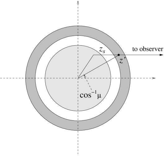
Figure 6.— Integration geometry for the ${}^{56}\mathrm{Ni}$ distribution form factor $q$. A ${}^{56}\mathrm{Co}$ gamma-ray is emitted from point $z$ in the region where $X_{{}^{56}\mathrm{Ni}}(z)>0$ (inner shaded region), and travels along the ray $z_{s}$ towards the observer. Point $z^{\prime}$ lies in a mass shell of thickness $dz^{\prime}$ (shaded annulus) in which the gamma-ray is trapped, scatters and deposits its energy.

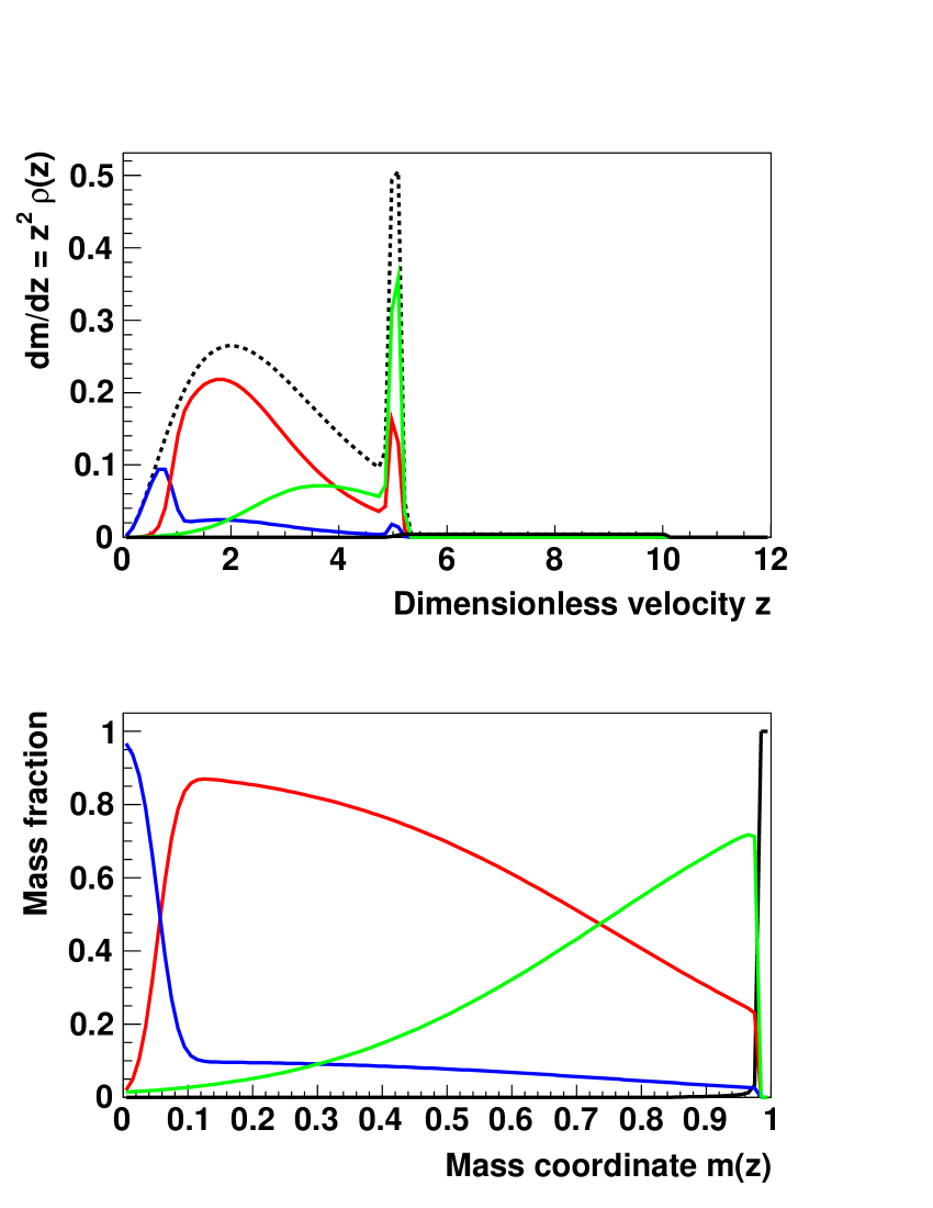
Figure 7.— Density and composition for an example model with $f_{\mathrm{Fe}}=0.12$, $f_{\mathrm{Ni}}=0.6$, $f_{\mathrm{sh}}=0.12$, $f_{\mathrm{env}}=0.02$. Top: Mass of a shell of ejecta of thickness $dz$ as a function of $z$. Black dotted line: overall density; solid lines, in rough order of increasing $z$: stable Fe-peak (blue), ${}^{56}\mathrm{Ni}$ (red), IME + unburned C/O (green), C/O envelope (black). Bottom: Composition of model as a function of mass coordinate $m(z)$.

Table 7Extracted model parameters

SN Name	$M_{\mathrm{tot}}/M_{\odot}~{}(>98\%)$	$M_{\mathrm{WD}}/M_{\odot}~{}(>98\%)$	$M_{\mathrm{Ni}}/M_{\odot}$	$f_{\mathrm{env}}$	$f_{\mathrm{sh}}$	$f_{\mathrm{Fe/sh}}~{}(<98\%)$	$\chi^{2}_{\nu}$	$P_{\mathrm{fit}}$
SNF 20070528-003	$2.04^{+0.47}_{-0.39}$ $(>1.49)$	$1.89^{+0.48}_{-0.41}$ $(>1.32)$	$0.91\pm 0.12$	$0.08\pm 0.05$	$0.30\pm 0.12$	$0.23^{+0.24}_{-0.14}~{}(<0.66)$	$1.08$	$0.290$
SNF 20070803-005	$1.57^{+0.18}_{-0.16}~{}(>1.32)$	$1.38^{+0.15}_{-0.13}~{}(>1.18)$	$0.75\pm 0.09$	$0.14\pm 0.03$	$0.40\pm 0.04$	$0.40^{+0.16}_{-0.12}~{}(<0.68)$	$0.69$	$0.654$
SN 2007if	$2.30^{+0.27}_{-0.24}~{}(>1.94)$	$1.98^{+0.21}_{-0.18}~{}(>1.70)$	$1.37\pm 0.13$	$0.16\pm 0.04$	$0.44\pm 0.05$	$0.63^{+0.17}_{-0.18}~{}(<0.85)$	$1.32$	$0.077$
SNF 20070912-000	$2.05^{+0.45}_{-0.39}$ $(>1.50)$	$1.90^{+0.46}_{-0.41}$ $(>1.33)$	$0.89\pm 0.15$	$0.09\pm 0.05$	$0.31\pm 0.12$	$0.22^{+0.25}_{-0.13}~{}(<0.66)$	$0.10$	$0.775$
SNF 20080522-000	$1.56^{+0.19}_{-0.14}~{}(>1.34)$	$1.45^{+0.17}_{-0.13}~{}(>1.25)$	$0.80\pm 0.11$	$0.08\pm 0.02$	$0.28\pm 0.04$	$0.33^{+0.15}_{-0.11}~{}(<0.59)$	$0.37$	$0.976$
SNF 20080723-012	$1.79^{+0.28}_{-0.21}~{}(>1.49)$	$1.69^{+0.25}_{-0.18}~{}(>1.41)$	$0.84\pm 0.11$	$0.06\pm 0.02$	$0.25\pm 0.05$	$0.24^{+0.12}_{-0.08}~{}(<0.45)$	$1.09$	$0.324$
SN 1991T	$1.65^{+0.22}_{-0.16}~{}(>1.39)$	$1.50^{+0.18}_{-0.13}~{}(>1.28)$	$0.77\pm 0.15$	$0.10\pm 0.03$	$0.34\pm 0.05$	$0.30^{+0.16}_{-0.11}~{}(<0.60)$	$0.83$	$0.600$
SN 2003fg	$2.31^{+0.30}_{-0.36}$ $(>1.77)$	$2.01^{+0.31}_{-0.36}$ $(>1.46)$	$1.18\pm 0.16$	$0.16\pm 0.07$	$0.44\pm 0.10$	$0.47^{+0.24}_{-0.21}~{}(<0.83)$	$0.09$	$0.945$

Note. — Quantities with error bars are marginalized over all independent parameters. Uncertainties are 68% CL ($1\sigma$) and represent projections of the multi-dimensional PDF onto the derived quantities. Upper or lower limits on poorly constrained properties are 98% CL.

To calculate $q$, we assume a density profile motivated by DET2ENVN which includes an envelope with density profile $\rho\sim z^{-2}$ on the outside, a thin Gaussian shell at $z_{\mathrm{sh}}=v_{\mathrm{sh}}/v_{e}$, and an exponential in velocity beneath the shell. The total density is given by

$$\rho(z) = C_{\mathrm{bulk}}\phi\left(\frac{z-z_{\mathrm{sh}}}{\sigma_{\mathrm{z,sh}}}\right)\exp(-z)+C_{\mathrm{env}}\phi\left(\frac{z_{\mathrm{sh}}-z}{\sigma_{\mathrm{z,sh}}}\right)z^{-2}$$ (8)

$$+ C_{\mathrm{sh}}\exp\left[-\frac{1}{2}\left(\frac{z-z_{\mathrm{sh}}}{\sigma_{\mathrm{z,sh}}}\right)^{2}\right],$$

where we choose $\phi(z)=\mathrm{erfc}(z/\sqrt{2})/2$ as a smooth function which approaches 1 for $z\ll-1$ and 0 for $z\gg+1$, and the constants $C_{\mathrm{bulk}}$, $C_{\mathrm{env}}$, $C_{\mathrm{sh}}$, are determined so that the mass fractions in each density profile component agree with the input values. Quimby et al. (2007) suggest a nominal width of 500 km s^-1 for the reverse-shock shell at velocity $v_{\mathrm{sh}}\sim 10000$ km s^-1. The self-similar shock interaction model of Chevalier et al. (1982) suggests that the reverse shock velocity width should be about 3% of the velocity at the contact discontinuity for an interaction with a $r^{-2}$ envelope and ejecta with a power-law density profile $r^{-n}$ with $n\sim 7$ (used to approximate SNe Ia in the context of interaction with a CSM wind, e.g., Wood-Vasey, Wang & Aldering, 2004). We assume a shell half-width of $\sigma_{\mathrm{z,sh}}=0.015z_{\mathrm{sh}}$ in line with Chevalier et al. (1982), although the expansion is homologous and no longer self-similar after the interaction. Our results are not sensitive to the exact value of $\sigma_{\mathrm{z,sh}}$; values in the range (0.01–0.05)$z_{\mathrm{sh}}$ give us the same value of $q$ to within 5% for reverse-shock shells with masses up to $0.5M_{\mathrm{WD}}$, and with much better agreement for less massive shells.

For $X_{{}^{56}\mathrm{Ni}}(z)$, we use a parametrized composition structure inspired by Kasen (2006):

$$X_{{}^{56}\mathrm{Ni}}(z) = \phi\left(\frac{m_{\mathrm{Fe,core}}-m(z)}{a_{\mathrm{Fe,core}}}\right)$$ (9)

$$\times \phi\left(\frac{m(z)-m_{\mathrm{IPE}}}{a_{\mathrm{IPE}}}\right)\times\max(\eta,0.9),$$

where $m(z)=\int_{0}^{z}z^{2}\tilde{\rho}(z)\,dz$ is the mass coordinate, and the stable Fe-peak core and the ${}^{56}\mathrm{Ni}$ mixing zone are bounded by mass coordinates $m_{\mathrm{Fe,core}}$ and $m_{\mathrm{IPE}}$ with mixing widths $a_{\mathrm{Fe,core}}$ and $a_{\mathrm{IPE}}$, respectively. This allows for some stable Fe-peak elements to be mixed throughout while maintaining a core in the innermost regions for high central density models (see Figure 7). For our modeling below we choose $a_{\mathrm{Fe}}=0.025$ and $a_{\mathrm{Ni}}=0.35$, so that the outward mixing of ${}^{56}\mathrm{Ni}$ corresponds roughly to the “enhanced mixing” case of Kasen (2006), in accordance with the behavior we see in the light curves. As the mass of the shell increases, the results may depend more sensitively on the particular distribution of ${}^{56}\mathrm{Ni}$ in the shell. We proceed with the analysis, but caution that more detailed models of the shock interaction, and/or actual hydrodynamic simulations of the explosion, may be needed to accurately understand gamma-ray transport for cases in which a large amount of ${}^{56}\mathrm{Ni}$ is swept up into the shell.

In general, the values of $q$ are higher for our SNe ($0.45\pm 0.05$) than the nominal $q=1/3$ value for a completely mixed exponential SN Ia, but there is very little variation with shell mass fraction. The mixing of ${}^{56}\mathrm{Ni}$ into a shell (and potentially above the photosphere) and the displacement of ${}^{56}\mathrm{Ni}$ to higher velocities by a stable Fe core have comparable effects on $q$, but the former effect is minimized in the “enhanced mixing” model characteristic of our light curves.

4.5. Modeling Results

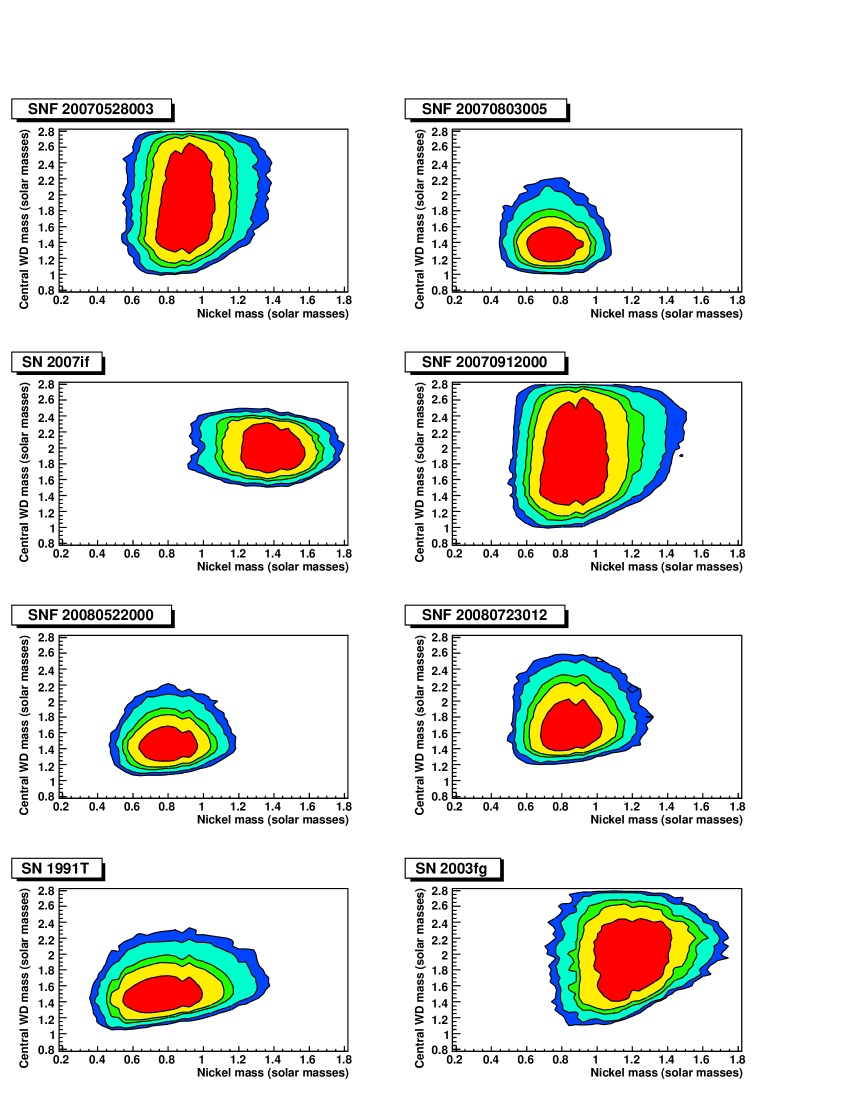
Figure 8.— Confidence regions in the $M_{\mathrm{WD}}$-${}^{56}\mathrm{Ni}$ mass plane for our six SNe, with priors $\alpha=1.3\pm 0.1$ and $\eta=0.90\pm 0.05$ as for DET2ENVN. SN 1991T and SN 2003fg are also shown. Contours bound regions of constant probability density. Colored regions are 68% (red), 90%, 95%, 99%, and 99.7% CL (blue).

The results of our modeling for the SNe in our sample are summarized in Table 7. Figure 8 shows the confidence regions in the $M_{\mathrm{WD}}$-${}^{56}\mathrm{Ni}$ mass plane for all six SNfactory SNe. While we limit our later statements about relative rates (see §5.4) and Hubble residuals (see §5.6) to the untargeted SNfactory search, which samples the smooth Hubble flow ($z>0.03$) and samples all host galaxy environments in an unbiased manner, we also include our results for two spectroscopically analogous SNe Ia from the literature as useful points of comparison: SN 1991T and SN 2003fg (see Appendix A).

Our results can be summarized as follows for the SNe in the SNfactory sample:

• We recover the results of Scalzo et al. (2010) for SN 2007if, within the uncertainties. The total system mass has come down slightly, from 2.41 $M_{\odot}$ to 2.30 $M_{\odot}$ (probability distribution median), since trapping of ${}^{56}\mathrm{Co}$ gamma-rays by the envelope is now included in the mass estimate. The fractions of the total system mass in the shell and in the envelope, set by the plateau velocity, remain the same.

• SNF 20070803-005 and SNF 20080522-000 are consistent with being Chandrasekhar-mass SNe Ia, albeit spectroscopically peculiar ones.

• SNF 20070528-003 and SNF 20070912-000 have data quality sufficient only to obtain lower limits on the total mass, and upper limits on the shell and envelope mass. In particular the lack of late-time photometry points mean that the lower limits are driven by the ${}^{56}\mathrm{Ni}$ mass from Arnett’s rule. The total system mass $M_{\mathrm{tot}}$, which includes the mass $M_{\mathrm{env}}$ of the envelope which we infer from the plateau velocity, is super-Chandrasekhar-mass at $>98\%$ confidence, although the mass $M_{\mathrm{WD}}$ of the central merger remnant is consistent with Chandrasekhar-mass values.

• SNF 20080723-012 appears to be a moderately super-Chandrasekhar-mass object, with ${}^{56}\mathrm{Ni}$ mass, total mass, and other parameters intermediate between SN 2007if and the rest of the population. We place a 98% CL lower limit of 1.41 $M_{\odot}$ on $M_{\mathrm{WD}}$, so that the progenitor system is likely super-Chandrasekhar-mass even without including $M_{\mathrm{env}}$.

We also perform the following cross-checks. First, our results are not strongly sensitive to the assumption of a particular mixing parameter, changing by less than 2% if we instead assume a completely stratified composition with $a_{\mathrm{Fe}}=a_{\mathrm{Ni}}=0$. Although changes in the mixing parameters do influence $q$ substantially for models with small amounts of ${}^{56}\mathrm{Ni}$, they matter much less when the ${}^{56}\mathrm{Ni}$ mass is large. We also confirm that when we discard the velocity information and fix $M_{\mathrm{env}}=0$, the resulting median reconstructed masses $M_{\mathrm{tot}}$ are within 2% of the median values of $M_{\mathrm{WD}}$, and the probability distributions have comparable widths. This is expected, since only the most massive envelopes (as in SN 2007if) make an appreciable contribution to the gamma-ray optical depth as seen from the inner layers of ejecta.

5. Discussion

We have shown that the subset of SNfactory events selected based on initial spectra similar to SN 2003fg, SN 2007if and SN 1991T can be fit well by a simple semi-analytic model of a tamped detonation, intended to describe the results of mergers of double-degenerate systems with total mass at or exceeding the Chandrasekhar limit. In the following section we explore results in the literature which can help us determine the extent to which this interpretation is unique and relevant.

In §5.1, we compare our observations to numerical models of SNe Ia with interacting shells in their ejecta, and to observations of SN 2005hj taken by Quimby et al. (2007). In §5.2, we evaluate the possibility that some of the luminosity of our events may be due to an ongoing shock interaction. In §5.3, we discuss other recent models of asymmetric, single-degenerate SN Ia explosions which attempt to reproduce the velocity plateau phenomenon, and their implications both for whether our SNe are super-Chandrasekhar and whether they are mergers. In §5.4, we present the relative rates and examine the extent to which our results may constrain merger scenarios if a significant number of SNe Ia have double-degenerate progenitors. In §5.5, we compare the aggregate probability distribution of total system mass from our events to population synthesis models of super-Chandrasekhar-mass double-degenerate mergers. Finally, in §5.6, we examine the deviation from the Hubble diagram for these SNe and discuss implications for SN Ia cosmology.

5.1. Comparison with Shell SN Ia Models in the Literature

Our most recent point of comparison in the literature for the application of explosion models with interacting shells to observations of SNe Ia is Quimby et al. (2007). They noted the presence of a velocity plateau in their observations of SN 2005hj and compared them to delayed detonation, pulsating delayed detonation and tamped detonation models (Khokhlov et al., 1993; Höflich & Khohklov, 1996; Gerardy et al., 2004).

For a shell mass fraction $f_{\mathrm{sh}}=0.07$, similar to our less extreme SNe, the predicted $B-V$ color is around 0.05-0.1. Quimby et al. (2007) note that the systematic uncertainty in the absolute value of $(B-V)_{\mathrm{max}}$ may be as large as 0.1 mag for the DET2ENVN models and other shell models. The color they report for SN 2005hj is $(B-V)_{\mathrm{max}}=0.04\pm 0.06$, consistent with the mean color in our sample, for a claimed shell mass fraction $f_{\mathrm{sh}}=0.14$, comparable to SNF 20070803-005.

According to Quimby et al. (2007) and references therein, one might expect to see cooler photospheres, and hence redder $(B-V)_{\mathrm{max}}$, with increasing shell mass fraction. Our modeling predicts that SN 2007if, with the lowest plateau velocity and the most massive progenitor, has the most massive shell in both absolute and relative terms. This SN may be somewhat redder than the others near maximum light, but the lack of light curve coverage near maximum makes it difficult to say exactly how much. Table 7 also shows that SN 2007if has the largest expected fraction of iron-peak elements in its shell, corresponding to the material near the photosphere around maximum light. To the extent that SN 2007if is intrinsically redder than our other SNe, this may be due in part to line blanketing by iron-peak elements, rather than a low-temperature photosphere, which would be inconsistent with the weakness of Si II $\lambda 5800$ in all the SNe in our sample.

While we cannot predict from theory how long the plateau phase should last without more sophisticated modeling of our SNe, the durations of our plateaus are also broadly consistent with expectations. For models of Chandrasekhar-mass events with envelope masses about 0.1 $M_{\odot}$(Quimby et al., 2007), the plateau phase is expected to last about 10 days. In most of our SNe it lasts at least 15 days (and at least 10 days for SNF 20070912-000). Quimby et al. (2007) derive a plateau duration of $20\pm 10$ days for SN 2005hj.

SNF 20080522-000 shows the longest-lived plateau in our data set, stretching as early as 10 days before $B$-band maximum and lasting as long as 30 days. A more conservative estimate would be that the plateau phase is confirmed to last from day $-3$, when Si II $\lambda 6355$ becomes strong enough that the error bars on the velocity of the absorption minimum drop below 500 km s^-1, to day $+15$, where Fe II lines begin to develop near Si II $\lambda 6355$ and blending may become a concern. All of our velocity measurements in this 18-day time window are contained in a narrow range just 250 km s^-1 wide.

5.2. Constraints on Ongoing Extended Emission

Fryer et al. (2010) ran three-dimensional smoothed-particle hydrodynamics (SPH) simulations of double-degenerate mergers. They found that the central merger remnants are indeed surrounded by an envelope with an approximate radial density profile $\rho(r)\propto r^{-\beta}$ with $3<\beta<4$. They then performed radiation hydrodynamics simulations of the interaction of the SN ejecta with the envelope, calculating synthetic spectra and light curves of the resulting explosions. For sufficiently massive envelopes (more massive than about 0.1 $M_{\odot}$), energy advected by the shock is released over the evolution of the SN, producing non-negligible luminosity near maximum light and extending emission into UV wavelengths. Based on these findings, Fryer et al. (2010) argued that these “enshrouded” systems would, in all likelihood, look nothing like SNe Ia. Blinnikov & Sorokina (2010) performed analogous calculations using the STELLA radiation hydrodynamics code, finding that in general a radial density profile as steep as $r^{-4}$ looked similar to a normal SN Ia in optical wavelengths ($UBVRI$), whereas a profile varying as $r^{-3}$ would be dominated by shock emission.

These findings put significant constraints on the radial extent and density profile of any envelope which might have enshrouded the progenitors of the SNe in our sample. In particular, the blue, mostly featureless spectrum seen in SN 2007if at phase $-9$ days is characteristic of what Fryer et al. (2010) expect, and the optical emission could be powered in part by advected heat energy from the shock interaction at early times, resulting in a broader light curve. However, the fact that $v$(Si II) in our events is seen to assume its plateau value as early as a week before maximum light, and the colors appear similar to those of normal SNe Ia near maximum light, argue strongly against any ongoing interaction with an extended envelope or wind.

As noted in Scalzo et al. (2010), if some fraction of the maximum-light luminosity is due to shock heating, whether advected or resulting from a fresh interaction, instead of ${}^{56}\mathrm{Ni}$ decay, our mass estimates would tend to increase. This is because the influence of the shock interaction would diminish substantially by about 50 days after explosion (Blinnikov & Sorokina, 2010), and more ${}^{56}\mathrm{Co}$ gamma rays would have to be trapped in order to reproduce the observed light curve. Any model in which shock heating produces a large amount of luminosity more than 50 days after explosion would probably not look like a SN Ia, and could not explain the appearance of the SNe Ia discussed in this paper.

One straightforward way to address the extent of any ongoing consequences of shock interactions in future studies would be to obtain early-phase UV light curves of a candidate super-Chandra SN Ia from a satellite such as Swift. The signature of any strong influence of shock heating would be evident therein.

5.3. Implications of Possible Asymmetry

The large inferred masses of our candidate super-Chandra SNe Ia, taken together with the observed plateaus in the Si II velocity, are both naturally explained by the tamped detonation model we put forth in this paper, and by the underlying double-degenerate merger scenario it represents. Some recent work, however, points towards the possibility of explaining these events in terms of asymmetric single-degenerate explosions.

Maeda et al. (2009, 2010a, 2010b, 2011) invoke large-angular-scale asymmetries to explain the diversity of velocity gradients observed in normal SN Ia explosions and the low/high velocity gradient (LVG/HVG) dichotomy (Benetti et al., 2005). They suggest that an asymmetric explosion may cause an overdensity in the ejecta on one side of the explosion, causing LVG behavior when viewed from that side, with the other side relatively less dense and exhibiting HVG behavior. Additionally, Hachisu et al. (2011) suggested that optically-thick winds blown from an accreting white dwarf could strip mass from the outer layers of its donor star, regulating the accretion rate and potentially allowing the white dwarf to accrete without exploding until reaching masses as large as 2.7 $M_{\odot}$. Such a white dwarf would have to rotate differentially, as in the models of Yoon & Langer (2005), with the attending uncertainty in the evolutionary history of such objects. If a differentially rotating white dwarf were to explode asymmetrically, this could present an explanation for our observations within the single-degenerate scenario. A scenario like this one, if correct, could also explain SN 2007if and the HVG SN 2009dc as being similar objects viewed from different angles. Tanaka et al. (2010) interpreted the low continuum polarization of SN 2009dc as evidence for a nearly spherical explosion, but low polarization could also be observed in an axisymmetric explosion viewed along the symmetry axis, as those authors note.

While we cannot at this time conclusively rule out the possibility that the Si II velocity plateaus we observe in our SNe result from asymmetry, no asymmetry is needed as yet to explain them, as argued e.g. by Maeda & Iwamoto (2009) for super-Chandrasekhar-mass explosions. The physical cause of the plateau — overdensity in the ejecta — is the same in symmetric and asymmetric models. If the velocity plateaus are indeed the result of asymmetric explosions, the shell mass fractions derived in Table 7 would still have meaning in terms of disturbances to the density structure along the line of sight, but the inferred envelopes would not be present, i.e., $M_{\mathrm{env}}$ would be zero and $M_{\mathrm{tot}}$ would equal $M_{\mathrm{WD}}$ for the SNe analyzed in this paper.

We can use the relative rate of supernovae spectroscopically similar to those in our sample (see §5.4 below) to make some general statements about how well they can be explained by lopsided asymmetric explosions. If the SNe Ia in our sample belonged to the same population as normal SNe Ia, and the spectroscopic peculiarity and brightness were due entirely to viewing angle effects (see Kasen, 2004, for an asymmetric model for which this is true), a relative rate of $\sim 2\%$ would imply a range of viewing angles no more than $\sim 15$ degrees from the symmetry axis. For models in which the asymmetry does not translate into a very peculiar spectrum, as seems likely for the Maeda et al. (2010b, 2011) models with high ${}^{56}\mathrm{Ni}$ mass, we should look instead at the diversity of velocity gradients among spectroscopic analogues. Since all of the (spectroscopically similar) SNe Ia in our sample have velocity gradients at the slowly-evolving extreme of what the model of Maeda et al. (2010b) claims to produce, it seems plausible that, within the context of this class of models, the density enhancements in the ejecta of our SNe are roughly isotropic.

Asymmetries resulting in overdensities in SN Ia ejecta along the line of sight could also affect gamma-ray trapping for that line of sight only. Most of the trapping happens in low-velocity ejecta (see §4.5), so the form factor $q$ should not be strongly affected; we think it unlikely that $q$, and our ejected mass estimates, could vary by more than 10%. Our ${}^{56}\mathrm{Ni}$ mass estimates from Arnett’s rule should also be robust, since according to Maeda et al. (2011), the effects of asymmetry on peak brightness are least pronounced for the most luminous SNe Ia. Based on these considerations and those of the preceding paragraph, the super-Chandrasekhar-mass status of SN 2007if and SNF 20080723-012 seems secure to us.

A different class of asymmetries might arise in bipolar, rather than lopsided, explosions. An axially symmetric merger geometry, featuring a disk of disrupted white dwarf material in the equatorial plane, could in principle result in velocity plateaus and peculiar spectra when viewed edge-on, but a more normal SN Ia appearance when viewed pole-on. This possibility was recently suggested by Livio & Pringle (2011), who also suggested that SNe Ia from merger events might show increasing diversity in their velocity gradients with increasing mass of carbon. In this scenario, SN 2009dc could be an event like SN 2007if viewed pole-on, consistent with its low continuum polarization (Tanaka et al., 2010); SN 2007if should then correspond to the edge-on case, and should show substantial polarization. Livio & Pringle (2011) make no predictions for relative rates in different SN Ia subgroups, which may depend on details of the hydrodynamic interaction of the SN ejecta with the disk. Nevertheless, an occluded region of ejecta narrow enough to explain their rare incidence would subtend only a small solid angle at the source, with only a small fraction of the ejecta decelerated. This would lead to broader, more complex line profiles than the ones we observe. It therefore once again seems reasonable that our SNe should be more or less spherically symmetric, with only moderate large-angular-scale asymmetries. Furthermore, any asymmetries compatible with our observations should influence only the inferred envelope masses $M_{\mathrm{env}}$, and should leave our estimates of $M_{\mathrm{WD}}$ intact at the 10% level, as we noted above.

Future observations, including nebular spectra of candidate super-Chandra SNe Ia for direct comparison with the abovementioned studies, may allow us to make more specific statements about their asphericity. Spectropolarimetry, as for SN 2009dc (Tanaka et al., 2010), may also be helpful.

5.4. Constraints on Merger Scenarios from Relative Rates

Mass modeling shows that all six of our SNfactory-discovered SNe Ia have a high probability of having super-Chandrasekhar-mass progenitors. Because ours was a wide-field search and our spectroscopy screening was conducted impartially, that is without pre-selection based on colors, luminosity, lightcurve shape, host galaxy environment etc., we may estimate the relative fraction of such objects.

A total of 400 spectroscopically-confirmed SNe Ia were discovered by the SNfactory. We did not spectroscopically screen candidates found to be fainter on the discovery image than on any pre-discovery detections that may have existed, as such candidates were assumed to be after maximum light. Furthermore, we did not perform spectroscopic screening in the cases where a host galaxy had a previously-known redshift beyond $z=0.08$, though such cases were rare.

We consider two subsamples — one that is purely flux-limited and another that is further limited to $z\leq 0.08$. For both subsamples we consider only SNe Ia discovered at or before maximum light, when the characteristic spectral features of SN 2003fg, SN 2007if and SN 1991T are clearest (Li et al., 2011). The flux-limit is represented by the survey efficiency as a function of magnitude rather than as a fixed magnitude. A subset redshift-limited to $z\leq 0.08$ is also considered as a cross-check, since here details of the survey efficiency become unimportant and the spectroscopic typing is very secure.

Among the super-Chandra candidates, all survive the pre-maximum and flux-limit cuts, while SNF 20070528-003 and SNF 20070912-000 are eliminated by the redshift cut. The sample cuts applied to the overall sample leave 240 SNe Ia in the flux-limited sample and 141 in the redshift-limited sample. Due to their enhanced brightness and generally longer rise times, the super-Chandra candidates are enhanced by factors of $1.30\pm 0.06$ and $1.11\pm 0.01$ in each of the two subsamples. These enhancements are calculated using the control time in the SNfactory search, accounting for both apparent magnitudes and light-curve widths of these SNe relative to normal SNe Ia. The assigned uncertainties are illustrative of the effect of a generous $\pm 0.25$ mag shift in the detection efficiency curve. As expected, this affect is small and has essentially no impact for the volume-limited subset. Including these correction factors, the rates are $1.9^{+1.1}_{-0.5}$% and $2.6^{+1.9}_{-0.7}$% for the flux-limited and redshift-limited subsamples, respectively. The difference in these relative rates is consistent with Poisson fluctuations, including accounting for the SNe Ia in common.

These are the relative rates under the assumption that all of our candidates have super-Chandrasekhar-mass progenitors, as their estimated masses under the tamped detonation model indicate. Alternatively, these can be taken as the rates for SNe Ia classified as like SN 1991T by using SNID. Although our 1.9–2.6% relative rate is somewhat lower than the “volume-limited” rate of $9.4^{+5.9}_{-4.7}$% (5-day cadence) from Li et al. (2011), we note that it is consistent with the $\sim 1\%$ “Ia-91T” rate of Silverman et al. (2012) from the same search. The difference between the two is related to how the events are classified. Li et al. (2011) use classifications from the IAU Circulars, rather than a homogeneous set of spectra over a given range of wavelengths and light-curve phases subclassified with a single method; in fact, Silverman et al. (2012) imply that some of the Li et al. (2011) subclassifications may be photometric (based on light-curve width) rather than spectroscopic. Li et al. (2011) also treat SNe with type “Ia-99aa” as being “Ia-91T’ rather than breaking them into separate subclasses, which led to their much higher rate. Using SNID, Silverman et al. (2012) classify only one of the Li et al. (2011) 1991T-likes (SN 2004bv) as “Ia-91T” and the rest as “Ia-99aa” or normal, leading to an updated “volume-limited” rate of $1.4^{+3.0}_{-0.0}$ for the Li et al. (2011) sample, consistent with our rate. As a point of comparison from an untargeted search similar to SNfactory’s, rather than a search targeting known galaxies, we also consider the SDSS spectroscopic sample (Östman et al., 2011). Seventy-eight of the 141 SNe Ia in the sample of Östman et al. (2011) have spectra with light-curve phases at or before maximum light, proof against the 1991T-like “age bias” (Li et al., 2011). Using SNID, Östman et al. (2011) type only two of these 78 as “Ia-91T”, leading to a relative rate of $3.4^{+2.4}_{-1.7}$%, again consistent with our own rate. We note that our rate estimates have considerably smaller uncertainty than these other 1991T-like SNe Ia rates. The combination of all three surveys, using our redshift-limited rates, gives a net 1991T-like rate of $2.3^{+1.2}_{-0.6}$%.

The statistical confidence intervals from our models indicate the possibility that not all candidates are super-Chandrasekhar-mass. The probability density extending below the Chandrasekhar mass represents the equivalent of 0.2 SNe Ia for both subsamples. If we correct for this excess probability, the rates are lowered by factors of 5% and 3% for the flux-limited and redshift-limited subsamples. A more precise correction would depend on the true parent mass distribution function, but it is evident from the above calculation that such details are well below the Poisson uncertainties.

Finally, we consider the rates under the possibility that the shell model is not appropriate. In this case there would be no contribution from the shell mass, and the best mass estimate would be that of the central merger remnant, $M_{\mathrm{WD}}$. In this circumstance SNF 20070803-005 and SNF 20080522-000 could be considered more likely to have been Chandrasekhar mass events. The rates resulting from their removal would then become $1.5^{+1.1}_{-0.4}$% and $1.0^{+1.4}_{-0.4}$%. While we view this situation as unlikely, for reasons discussed above in §5.3, the rates remain dominated by Poisson uncertainties rather than modeling assumptions.

These relative rates are very low. Therefore, if double-degenerate mergers are to contribute significantly to the total SN Ia rate, most such mergers would need to escape our spectroscopic selection. Moreover, the SNfactory has not found overluminous SNe Ia in addition to those presented here or SN 2005gj (Aldering et al., 2006) that would qualify for our redshift-limited sample.

While our events are overluminous with large ${}^{56}\mathrm{Ni}$ masses, theoretical mergers (Pakmor et al., 2011, 2012, e.g.) thus far predict a range of smaller ${}^{56}\mathrm{Ni}$ masses, resulting in fainter explosions with lower photospheric temperatures. As discussed in §5.2 above, a delay in the release of radiant energy from a shock interaction could also contribute to heating the photosphere at early times in events like SN 2007if, so that mergers with less massive envelopes would have more normal spectra.

Merger events with less massive envelopes should also have less disturbed density structures, and hence may not display the low Si II velocity plateau behavior we observe in our sample. The small envelope mass fractions implied for the majority of merger events would then represent a constraint on either the dynamics of the merger in the case of a prompt explosion, or the post-merger evolution of the system in the case of a delayed explosion triggered by accretion onto, or by post-accretion spin-down of, the central merger remnant. Unambiguous detection of a density enhancement signature for less massive shells would be difficult. Construction of their mass distribution function would require a parent sample of SNe Ia all followed spectroscopically such that any merger candidates could be selected by their velocity plateau behavior rather than spectroscopic peculiarity. Moreover, such a study would require spectra at very early phases ($-10$ days or younger), since a less massive reverse-shock shell would become transparent at earlier phases, and might not subsume most of the intermediate-mass elements in the explosion.

Determining the relative importance of any of these factors, and thus understanding the true relation of candidate super-Chandra SNe Ia to the general SN Ia population, will require further work and new spectroscopic data sets. However, we can say that a range of envelope masses are probably needed to explain the range of plateau velocities we observe in our data.

5.5. Progenitor Mass Distribution in the Double-Degenerate Scenario

Figure 9 presents the aggregate PDF of the masses of the SNe in our sample, each weighted inversely by their control time in the SNfactory search, accounting for both apparent magnitude and light-curve width. Its lower edge is roughly consistent with the Chandrasekhar mass, with a tail towards higher masses.

This distribution is qualitatively similar to expectations for super-Chandrasekhar-mass merging white dwarf system masses from population synthesis models (Ruiter et al., 2009; Fryer et al., 2010). The limited statistics and theoretical uncertainties make it difficult to draw a firm, quantitative correspondence between observations and theory, but we can nevertheless look for gross inconsistencies. Figure 9 therefore also includes three theoretical distributions of the progenitor system mass ($M_{\mathrm{tot}}$) shown in Fryer et al. (2010), cut off below 1.4 $M_{\odot}$ and convolved with a two-sided Gaussian ($\sigma_{-}=0.08\,M_{\mathrm{tot}}$, $\sigma_{+}=0.10\,M_{\mathrm{tot}}$) to model our reconstruction precision.

Our observations correspond well with the Ruiter et al. (2009) models on the leading edge, particularly the $\gamma=1.5$ model. The differences are more pronounced on the high-mass tail; the agreement may improve with a larger sample of SNe. The other two models agree less well, predicting more high-mass mergers than we see in our sample. In the $\gamma=1.5$ model, the relative rate of events $dN/dM_{\mathrm{tot}}$ is about a factor of 3 higher at 1.4 $M_{\odot}$ than at 2.1 $M_{\odot}$, consistent with our observations. The other two models predict more high-mass mergers than we observe; we see no evidence for a separate formation channel or peak near 2 $M_{\odot}$ as suggested by Fryer et al. (2010). If such massive mergers do exist, they must therefore produce less ${}^{56}\mathrm{Ni}$, and be less luminous at maximum light, than the SNe in our sample.

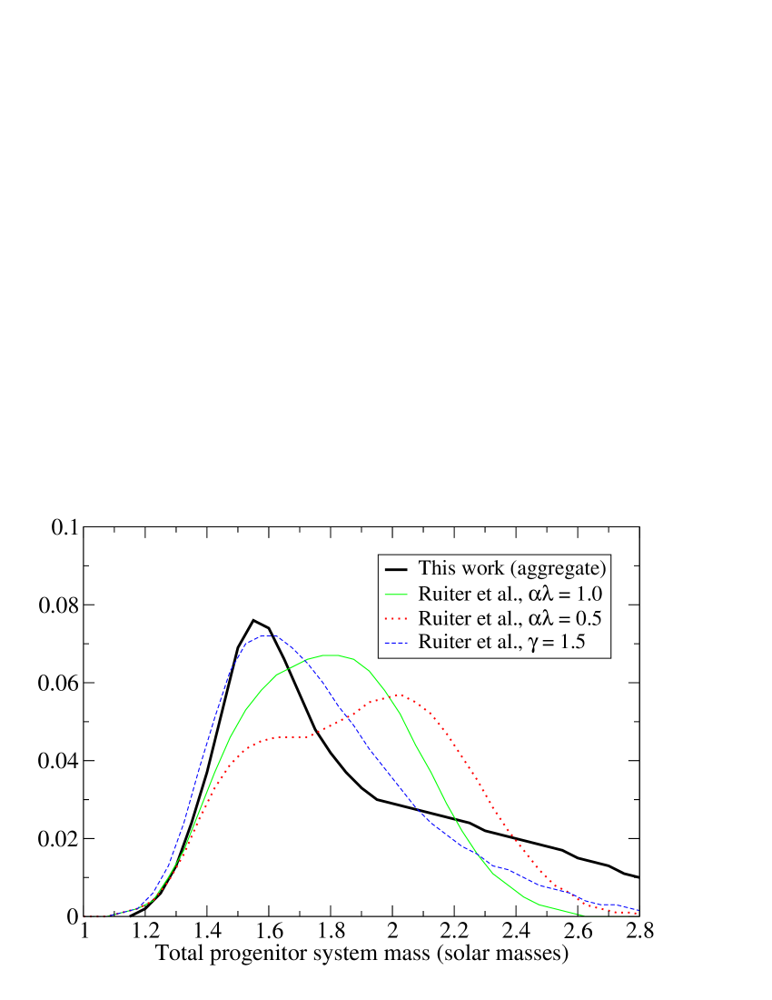
Figure 9.— Total progenitor mass PDF for our sample (thick solid line), compared with various population synthesis models of Ruiter et al. (2009) as shown in Fryer et al. (2010): $\alpha\lambda=1.0$ (thin solid line), $\alpha\lambda=0.5$ (dotted line), and $\gamma=1.5$ (dashed line). Population synthesis models have been cut off below 1.4 $M_{\odot}$ and convolved with the mass resolution of our reconstruction technique, then normalized to match our total event rate.

5.6. Hubble Residuals and Implications for Cosmology

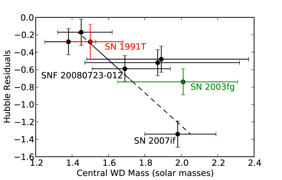
Figure 10.— Hubble residuals vs. central merger remnant mass for our sample (black points). SN 1991T (red) and SN 2003fg (green) are also plotted for comparison. Error bars are 68% ($1\sigma$) uncertainties. The dotted black line is the best-fit linear trend.

Table 3 also contains the Hubble residuals of each SN in our sample from a standard $\Lambda$CDM cosmology:

$$\Delta\mu=m_{B}-25-5\,\log_{10}(d_{L}/\mathrm{Mpc})-\alpha(s-1)+\beta c-M_{B},$$ (10)

where $m_{B}$, $s$ and $c$ are derived from the SALT2 fits, $d_{L}$ is calculated using Wright (2006), and we use values of $\alpha$, $\beta$, and $M_{B}$ from the $w=-1$ fit of Sullivan et al. (2011). (We use $M_{B}=M^{1}_{B}$, i.e., the absolute magnitude appropriate for SNe in host galaxies with stellar mass less than $10^{10}~{}M_{\odot}$.)

Figure 10 plots the relation $\Delta\mu$ vs. $M_{\mathrm{WD}}$ (instead of $M_{\mathrm{tot}}$, so that it does not depend on interpreting the velocity plateau in terms of an envelope) for the six SNfactory SNe Ia. For comparison we also plot SN 1991T and SN 2003fg, modeled in a similar fashion (see Appendix A). The Hubble residuals show a correlation with increasing mass (Pearson $r=-0.76$, $p=0.03$). SN 2007if is 1.3 mag overluminous for its stretch and color, and by 1 mag even if no correction is made for its redder-than-average color. SNF 20080723-012 is about 0.6 mag too luminous for its stretch and color, putting it off the Hubble diagram but to a lesser degree than SN 2007if. At the low-mass end, SNF 20070803-005 and SNF 20080522-000, while slightly overluminous, are not alarmingly discrepant, being within two standard deviations of the $\Lambda$CDM Hubble diagram assuming an intrinsic dispersion of 0.15 mag. The higher-redshift ($z\sim 0.12$) SNF 20070528-003 and SNF 20070912-000 are too luminous for their stretch and color by about 0.5 mag; the residual decreases to about 0.4 mag if no correction is made for the color.

If the correlation shown in Figure 10 is real, and the large Hubble residuals of SN 2003fg and SN 2007if are related to their large progenitor masses, the large Hubble residuals of SNF 20070528-003 and SNF 20070912-000 provide further circumstantial evidence that they too may have super-Chandrasekhar-mass progenitors. One might expect deviations of super-Chandra candidate SNe Ia from the width-luminosity relation for normal SNe Ia, either because the large ejected mass could increase the diffusion time of radiation through the ejecta relative to Chandrasekhar-mass explosions, or because the enhanced mixing of ${}^{56}\mathrm{Ni}$ into the outer layers of ejecta in these events affects the ionization state at the photosphere (see Kasen & Woosley, 2007, and references therein).

Previous authors have warned about overluminous SNe Ia that could skew the cosmological parameters. Reindl et al. (2005) found that the SN 1991T subclass give a mean Hubble residual of $-0.4$ mag. The sample presented here has a mean Hubble residual is $-0.56$ mag, dropping to $-0.41$ mag if SN 2007if were excluded on the grounds that it would be easy to eliminate. However, without a spectroscopic veto at high redshift, or by relying only on photometry at any redshift, it will be difficult to tag and remove SNe such as these from the Hubble diagram. Although SN 2007if is excessively overluminous and would probably be excluded from any Hubble diagram on that basis, somewhat less luminous analogues like SNF 20080723-012 probably could not be safely removed based on their overluminosity alone. It would also be difficult, without spectroscopy, to distinguish intrinsically overluminous SNe Ia from normal SNe Ia magnified by gravitational lensing; since lensing conserves photons in general relativity (Weinberg, 1976), all events must be included on the Hubble diagram to avoid bias in the reconstructed cosmological parameters.

Suppose candidate super-Chandra SNe Ia occur at the relative rate we calculate for our redshift-limited subsample in §5.4 ($2.6^{+1.9}_{-0.7}$) and have a mean Hubble diagram residual of $-0.41$ mag, the mean of the Table 3 entries excluding SN 2007if. The mean absolute magnitude of SNe Ia is then 0.01–0.02 mag higher (68% CL) than it would be if these SNe followed the normal relations. This number is already comparable to the 2% error budget suggested in Kim et al. (2004) for Stage IV SN Ia cosmology experiments, and would be realized if the rate evolves by either doubling or going to zero at high redshift.

6. Conclusions

We have observed a sample of SNe Ia which we selected on the basis of their pre-maximum similarity to SN 2007if, searching for new candidate super-Chandra SNe Ia. Based on these spectroscopic analogues, we find that SN 2007if probably lies on the extreme luminous end, with a hot, highly ionized photosphere and a disturbed density structure resulting from a stalled shock within the ejecta. We interpret these characteristics as evidence for an interaction with a circumstellar envelope early in the SN’s evolution, as one might expect in a double-degenerate merger scenario.

To reconstruct the masses of the progenitors, we apply an updated version of the modeling technique of Scalzo et al. (2010). By applying this technique to SN 1991T for comparison with Stritzinger et al. (2006), we show that including NIR flux near phase $+40$ days as part of the bolometric flux has a significant impact on the final reconstructed mass; while there is some uncertainty associated with correcting for NIR flux not actually observed, ignoring such a correction causes the mass to be systematically underestimated. Our modeling technique includes a set of Bayesian priors motivated by theoretical models, capturing the covariance between different parameters of the system, and we sample the full probability distribution using a Monte Carlo Markov chain. From our sample, SNF 20080723-012 now joins SN 2007if in having a super-Chandrasekhar-mass progenitor at high statistical confidence. The mean error-weighted system mass for the four remaining SNe in our sample ($1.63~{}M_{\odot}\pm 0.10~{}M_{\odot}$) is also above the Chandrasekhar mass at a statistical confidence level exceeding 99%.

Although the spectrophotometric observations discussed here are quite detailed, with excellent temporal and wavelength coverage, the modeling presented is relatively simple and is meant to explore a large parameter space of rudimentary explosion models quickly and efficiently. Detailed comparison of the spectra to synthetic spectra of a range of contemporary explosion models will be necessary to determine the extent to which our modeling faithfully represents the density structure found in these SNe. Our simple model also assumes spherical symmetry of the SN ejecta, and this approximation may not hold true in a significantly aspherical merger scenario. The shell mass estimates must necessarily be subject to systematic uncertainties of this sort, and hence might be more properly construed as upper limits for which equality holds in the case of spherical symmetry. The total mass estimates, which concern the bulk ejecta and not only the outer layers, should be more robust.

Further study of a larger sample of such SNe Ia may provide additional insight into both the explosions themselves and the formation of their progenitor systems, particularly the extent to which velocity plateaus are linked to super-Chandrasekhar-mass progenitors. Future data sets including not only optical-wavelength observations, but infrared observations and nebular spectra, can help to verify the luminosity, ${}^{56}\mathrm{Ni}$ content and distribution, and total mass of these events. Ultraviolet and X-ray observations of SNe Ia spectroscopically similar to SN 1991T at early phase may also help to constrain the contribution of prompt shock emission to their luminosity, and the density and spatial extent of any envelope of material that might surround their progenitors just prior to explosion. Polarimetry and spectropolarimetry, as well as velocity offsets measured from nebular spectra, can help constrain the degree of large-angular-scale asymmetry. Finally, similar analysis of a much larger SN Ia data set may help to discover super-Chandrasekhar-mass SNe Ia whose spectroscopic appearance is unlike those in our sample; this may help to clarify the connection of these events to the general SN Ia population, with dividends paid to the understanding of SN Ia progenitors and to the precision of SN Ia cosmology.

Appendix A Mass Modeling of Spectral Archetypes

In addition to SN 2007if, SN 2003fg and SN 1991T are spectroscopic archetypes for the candidate super-Chandra SNe Ia presented in this paper. Thus, in order to have self-consistent mass estimates for the full archetype set and provide the reader with familiar points for comparison, we have applied our modeling procedure to SN 199T and SN 2003fg.

A.1. SN 1991T

SN 1991T is the most well-known spectroscopic archetype of our sample, although not the most spectroscopically extreme example. SN 1991T has good wavelength coverage in published spectra taken between maximum light and phase $+40$ days, allowing us to use the same analysis techniques as for the rest of our sample. In addition, modeling of SN 1991T allows a useful direct comparison to the earlier work of Stritzinger et al. (2006).

SN 1991T’s remarkably flat velocity evolution was pointed out by Phillips et al. (1992), and it has the second-lowest velocity gradient $\dot{v}$ in the original sample of Benetti et al. (2005). The DET2ENV2 model fits SN 1991T (Höflich & Khohklov, 1996), and indeed SN 1991T was once suspected to have had a super-Chandrasekhar-mass progenitor, mostly because of its high luminosity (Fisher et al., 1999). Later measurements of the distance (Richtler et al., 2001; Gibson & Stetson, 2001) to the host galaxy, NGC 4527, have decreased the SN’s luminosity considerably, and hence its inferred mass.

We can make a new estimate of the progenitor mass of SN 1991T using our reconstruction method, which considers the gamma-ray trapping in more detail than previous studies. We use the $BVRI$ light curve of Lira (1998) and the spectral time series of Mazzali et al. (1995) obtained through the SUSPECT online supernova spectrum archive. Kanbur et al. (2003) give the Cepheid-based distance modulus to NGC 4527, after correction for metallicity, as $30.71\pm 0.13$ (LMC period-luminosity relation) and $30.78\pm 0.13$ (Milky Way period-luminosity relation), We adopt the mean of these two measurements ($30.74\pm 0.13$) for our work. From a joint fit to the spectral time series we extract $EW$(Na I D)$=0.84\pm 0.18$ Å, giving $E(B-V)_{\mathrm{host}}=0.13\pm 0.03$ from the shallow TBC relation, in good agreement with the estimates of Phillips et al. (1992) and Phillips et al. (1999). Our model represents a good fit to the available data, with $\chi^{2}_{\nu}=0.83$ ($P_{\mathrm{fit}}=0.60$). We recover a ${}^{56}\mathrm{Ni}$ mass of $0.77\pm 0.15$ $M_{\odot}$ and a white dwarf mass $1.50^{+0.18}_{-0.13}$ $M_{\odot}$. If we suppose that the plateau is caused by interaction with a uniform spherical carbon/oxygen envelope, this envelope has a mass of about 0.1 $M_{\mathrm{WD}}$, and the total system mass estimate goes up to $1.65^{+0.22}_{-0.16}$ $M_{\odot}$. The results are similar to those for the nominal Chandrasekhar-mass SNe in our sample, SNF 20070803-005 and SNF 20080522-000.

Stritzinger et al. (2006) measured a mass of $1.21\pm 0.36$ $M_{\odot}$ for SN 1991T. Our median derived mass for SN 1991T exceeds that of Stritzinger et al. (2006) by over 0.4 $M_{\odot}$; our 98% CL lower limit on $M_{\mathrm{WD}}$ is 1.28 $M_{\odot}$. However, we find that we can reproduce Stritzinger et al. (2006)’s numbers for $t_{0}$, ${}^{56}\mathrm{Ni}$ mass, and ejected mass if we neglect NIR corrections and ignore covariances in our fitting procedure, particularly that between $q$ and $v_{e}$. In particular, by including NIR corrections we find $t_{0}=48$ days, much larger than the Stritzinger et al. (2006) value of 34 days and suggesting more massive ejecta. Our larger median value for $q$ (0.42) and slightly lower $v_{e}$ (2850 $\mathrm{km~{}s}^{-1}$) pull in the other direction, resulting in a mass closer to the the Chandrasekhar mass.

In summary, SN 1991T shows the observational hallmarks of a tamped detonation and may well have been a double-degenerate merger. Because of uncertainties in the host distance and reddening correction, we are unable to establish with confidence whether SN 1991T was itself super-Chandrasekhar-mass.

A.2. SN 2003fg

SN 2003fg (Howell et al., 2006) has a comparatively limited data set for our purposes, with only one spectrum at maximum light and no photometry at sufficiently late times for us to constrain the gamma-ray transparency. Nevertheless, there are noted similarities to SN 2007if: The single spectrum available is a good match to SN 2007if at a comparable phase, though with stronger Si II and S II. The observed $i^{\prime}$-band light curve of SN 2003fg shows no significant inflection, like SN 2007if and unlike the less massive SNfactory SNe Ia. The low ($\sim 8000~{}\mathrm{km~{}s}^{-1}$) Si II velocity near maximum light is also like SN 2007if at similar phases, and makes SN 2003fg a good candidate for a tamped detonation, although SN 2009dc showed a similarly low velocity without a discernable plateau (Yamanaka et al., 2009).

We can obtain a lower limit on the mass of SN 2003fg assuming it can be fit by a tamped detonation. We use the value of the bolometric absolute magnitude at maximum light ($M_{\mathrm{bol}}=-19.87$) and the velocity of the Si II $\lambda 6355$ absorption minimum ($\sim 8000\pm 500~{}\mathrm{km~{}s}^{-1}$) derived by Howell et al. (2006). Assuming no host galaxy reddening, we find a ${}^{56}\mathrm{Ni}$ mass of $1.18\pm 0.16~{}M_{\odot}$ and a 98% CL lower limit on the total system mass of $1.77M_{\odot}$ ($1.46~{}M_{\odot}$ if the envelope mass is neglected). These are somewhat looser constraints than those of Howell et al. (2006), but are free of the assumption that the photospheric velocity should be related directly to the kinetic energy released in the explosion, which, as we have seen, may not be a good approximation for some density structures.

References

- Aldering et al. (2002) Aldering, G., Adam, G., Antilogus, P., et al. 2002, Proc. SPIE, 4836, 61
- Aldering et al. (2006) Aldering, G., Antilogus, P., Bailey, S., et al. 2006, ApJ, 650, 510
- Arnett (1982) Arnett, W. D. 1982, ApJ, 253, 785
- Bacon et al. (1995) Bacon, R., Adam, G., Baranne, A., et al. 1995, A&AS, 113, 347
- Bacon et al. (2000) Bacon, R., Emsellem, E., Copin, Y., et al. 2000, in ASP Conf. Ser. 195, Imaging the Universe in Three Dimensions, ed. W. van Breugel & J. Bland-Hawthorn (San Francisco: ASP), 173
- Bacon et al. (2001) Bacon, R., Copin, Y., Monnet, G., et al. 2001, MNRAS, 326, 23
- Bailey et al. (2009) Bailey, S., Aldering, G., Antilogus, P., et al. 2009, A&A, 500, L17
- Baltay et al. (2007) Baltay, C., Rabinowitz, D., Andrews, P., et al. 2007, PASP, 119, 1278
- Benetti et al. (2005) Benetti, S., Cappellaro, E., Mazzali, P., et al. 2005, ApJ, 623, 1011
- Bessell (1990) Bessell, M. S. 1990, PASP, 102, 1181
- Blinnikov & Sorokina (2010) Blinnikov, S. I. & Sorokina, E. I. 2010, arXiv:1009.4353
- Blondin & Tonry (2007) Blondin, S., & Tonry, J. L. 2007, ApJ, 666, 1024
- Blondin et al. (2011) Blondin, S., Kasen, D., Roepke, F., et al. 2011, MNRAS, 417, 1280
- Bloom et al. (2012) Bloom, J. S., Kasen, D., Shen, K. J., et al. 2012, ApJ, 744, L17
- Bongard et al. (2011) Bongard, S., Soulez, F., Thiébaut, É. et al. 2011, MNRAS, 418, 258
- Branch et al. (1993) Branch, D., Fisher, A., & Nugent, P. 1993, AJ, 106, 2383
- Branch & Khokhlov (1995) Branch, D., & Khokhlov, A. M. 1995, Phys. Rep., 256, 53
- Branch et al. (2003) Branch, D., Baron, E. A., & Jeffery, D. A. 2003, in LNP 598, Supernovae and Gamma-Ray Bursters, ed. K. Weiler. (Berlin: Springer), 47
- Cardelli et al. (1988) Cardelli, J. A., Clayton, G. C. & Mathis, J. S. 1988, ApJ, 329, L33
- Chevalier et al. (1982) Chevalier, R. 1982, ApJ, 258, 790
- Childress et al. (2011) Childress, M. J. 2011, ApJ, 733, 3
- Conley et al. (2006) Conley, A., Howell, D. A., Howes, A., et al. 2006, AJ, 132, 1707
- Contardo, Leibundgut & Vacca (2000) Contardo, G., Leibundgut, B., & Vacca, W. D. 2000, A&A, 359, 876
- Di Stefano (2010a) Di Stefano, R. 2010, ApJ, 712, 728
- Di Stefano (2010b) Di Stefano, R. 2010, ApJ, 719, 474
- Di Stefano & Kilic (2012) Di Stefano, R. & Kilic, M. 2012, ApJ, submitted (arXiv:1205.3168)
- Filippenko et al. (1992) Filippenko, A. V., Richmond, M. W., Matheson, T., et al. 1992, ApJ, 384, L15
- Fisher et al. (1999) Fisher, A., Branch, D., Hatano, K., et al. 1999, MNRAS, 304, 67
- Fisher (2000) Fisher, A. 2000, Ph.D. thesis, University of Oklahoma
- Folatelli et al. (2009) Folatelli, G., Phillips, M. M., Burns, C., R., et al. 2010, AJ, 139, 120
- Foley & Kasen (2011) Foley, R. J. & Kasen, D. 2010, ApJ, 729, 55
- Foley et al. (2011) Foley, R. J., Sanders, N. E., & Kirshner, R. P. 2011, ApJ, 742, 89
- Fryer et al. (2010) Fryer, C. L., Ruiter, A. J., Belczynski, K., et al. 2010, ApJ, 725, 296
- Ganeshalingam et al. (2011) Ganeshalingam, M., Li, W., & Filippenko, A. V. 2011, MNRAS, 416, 2607
- Gerardy et al. (2004) Gerardy, C. L., Höflich, P., Fesen, R. A., et al.2004, ApJ, 607, 391
- Goldhaber et al. (2001) Goldhaber, G., Groom, D. E., Kim, A. G., et al. 2001, ApJ, 558, 359
- Gibson & Stetson (2001) Gibson, B. K. & Stetson, P. B. 2001, ApJ, 547, L103
- Gilfanov & Bogdan (2010) Gilfanov, M. & Bogdan, A. 2010, Nature, 463, 924
- Guy et al. (2007) Guy, J., Astier, P., Baumont, S., et al. 2007, A&A, 466, 11
- Guy et al. (2010) Guy, J., Sullivan, M., Conley, A., et al. 2010, A&A, 523, 7
- Hachisu et al. (2010) Hachisu, I., Kato, M., & Nomoto, K. 2010, ApJ, 724, L212
- Hachisu et al. (2011) Hachisu, I., Kato, M., Saio, H., et al.2012, ApJ, 744, 69
- Hicken et al. (2007) Hicken, M., Garnavich, P. M., Prieto, J. L., et al. 2007, ApJ, 669, L17
- Hillebrandt et al. (2007) Hillebrandt, W., Sim, S. A., & Röpke, F. K. 2007, A&A, 465, L17
- Höflich & Khohklov (1996) Höflich, P. & Khohklov, A. 1996, ApJ, 457, 500
- Howell et al. (2005) Howell, D. A., Sullivan, M., Perrett, K., et al. 2005, ApJ, 634, 1190
- Howell et al. (2006) Howell, D. A., Sullivan, M., Nugent, P. E., et al. 2006, Nature, 443, 308
- Howell et al. (2009) Howell, D. A., Sullivan, M., Brown, E. F., et al. 2009, ApJ, 691, 661
- Iben & Tutukov (1984) Iben, I. & Tutukov, A. V. 1984, ApJS, 54, 335
- Jeffery & Branch (1990) Jeffery, D. J., & Branch, D. 1990 in Supernovae, Jerusalem Winter School for Theoretical Physics ed. J. C. Wheeler, T. Piran, & S. Weinberg (Singapore: World), 149
- Jeffery (1999) Jeffery, D. J. 1999, arXiv:astro-ph/9907015
- Jeffery et al. (2006) Jeffery, D. J., Branch, D. & Baron, E. 2006, arXiv:astro-ph/0609804
- Justham (2011) Justham, S. 2011, ApJ, 730, L34
- Kanbur et al. (2003) Kanbur, S. M., Ngeow, C., Nikolaev, S., et al. 2003, A&A, 411, 361
- Kasen (2004) Kasen, D., Nugent, P., Thomas, R. C., et al. 2004, ApJ, 610, 876
- Kasen (2006) Kasen, D. 2006, ApJ, 649, 939
- Kasen & Woosley (2007) Kasen, D. & Woosley, S. E. 2007, ApJ, 656, 661
- Khan et al. (2011) Khan, A., Müller, E. & Höflich, P. Khan, R., Stanek, K. Z., Stoll, R., & Prieto, J. L. 2011, ApJ, 737, L24
- Khokhlov et al. (1993) Khokhlov, A., Müller, E. & Höflich, P. 1993, A&A, 270, 223
- Kim et al. (2004) Kim, A. G., Linder, E. V., Miquel, R., et al. 2004, MNRAS, 347, 909
- Krueger et al. (2010) Krueger, B. K. Jackson, A. P., Townsley, D. M., et al.2010, ApJ, 719, L5
- Landolt (1992) Landolt, A. U. 1992, AJ, 104, 340
- Lantz et al. (2004) Lantz, B., Aldering, G., Antilogus, P., et al. 2004, Proc. SPIE, 5249, 146
- Li et al. (2011) Li, W., Leaman, J.; Chornock, R., et al.2011, MNRAS, 412, 1441
- Li et al. (2011) Li, W., Bloom, J. S., Podsiadlowski, P., et al. 2011, Nature, 480, 348
- Linder (2006) Linder, E. V. 2006, Phys. Rev. D, 74, 103518
- Lira (1998) Lira, P., Suntzeff, N. B., Phillips, M. M., et al. 1998, AJ, 115, 234
- Livio & Pringle (2011) Livio, M., & Pringle, J. E. 2011, ApJ, 740, 18
- Maeda et al. (2009) Maeda, K., Kawabata, K., Li, W., et al. 2009, ApJ, 690, 1745
- Maeda & Iwamoto (2009) Maeda, K., & Iwamoto, K. 2009, MNRAS, 394, 239
- Maeda et al. (2010a) Maeda, K., Taubenberger, S., Sollerman, J., et al. 2010, ApJ, 708, 1703
- Maeda et al. (2010b) Maeda, K., Benetti, S., Stritzinger, M., et al. 2010, Nature, 466, 82
- Maeda et al. (2011) Maeda, K., Leloudas, S., Taubenberger, S., et al. 2011, MNRAS, 413, 3075
- Mazzali et al. (1995) Mazzali, P. A., Danziger, I. J., & Turatto, M. 1995, A&A, 297, 509
- Miller (1993) Miller, J. S., & Stone, R. P. S. 1993, Lick Observatory Technical Reports, No. 66 (Santa Cruz, CA: Lick Obs.)
- Nadyozhin (1994) Nadyozhin, D. K. 1994, ApJS, 92, 527
- Nomoto et al. (1984) Nomoto, K., Thielemann, F.-K., & Yokoi, K. 1984, ApJ, 286, 644
- Nomoto & Kondo (1991) Nomoto, K. & Kondo, Y. 1991, ApJ, 367, L19
- Nugent et al. (1995) Nugent, P., Branch, D., Baron, E., et al. 1995, Phys. Rev. Lett., 75, 394
- Nugent et al. (2002) Nugent, P. E., Kim, A. G., & Perlmutter, S. 2002, PASP, 114, 803
- Nugent et al. (2011) Nugent, P., Sullivan, M., Cenko, S. B., et al. 2011, Nature, 480, 344
- Oke et al. (1995) Oke, J. B., Cohen, J. G., Carr, M., et al. 1995, PASP, 107, 375
- Östman et al. (2011) Östman, L. et al.2011, A&A, 526, A28
- Pakmor et al. (2011) Pakmor, R., Hachinger, S., Röpke, F., et al.2011, A&A, 528, 117
- Pakmor et al. (2012) Pakmor, R., Kromer, M., Taubenberger, S., et al.2012, ApJ, 747, L10
- Perlmutter et al. (1999) Perlmutter, S., Aldering, G., Goldhaber, G., et al. 1999, ApJ, 517, 565
- Pfannes et al. (2010a) Pfannes, J. M. M. Niemeyer, J., Schmidt, W., et al. 2010, A&A, 509, 74
- Pfannes et al. (2010b) Pfannes, J. M. M. Niemeyer, J., & Schmidt, W. 2010, A&A, 509, 75
- Piro (2008) Piro, A. 2008, ApJ, 679, 616
- Phillips et al. (1992) Phillips, M. M., Wells, L. A., Suntzeff, N. B., et al. 1992, AJ, 103, 1632
- Phillips et al. (1999) Phillips, M. M., Lira, P., Suntzeff, N. B., et al. 1999, AJ, 118, 1766
- Poznanski et al. (2011) Poznanski, D., Ganeshalingam, M., Silverman, J. M., et al. 2011, MNRAS, 415, 81
- Quimby et al. (2007) Quimby, R. M., Höflich, P., & Wheeler, J. C. 2007, ApJ, 666, 1083
- Raskin et al. (2010) Raskin, C., Scannapieco, E., Rockefeller, G., et al. 2010, ApJ, 724, 111
- Reindl et al. (2005) Reindl, B., Tammann, G. A., Sandage, A., et al. 2005, ApJ, 624, 532
- Richtler et al. (2001) Richtler, T., Jensen, J. B., Tonry, J., et al. 2001, A&A, 368, 391
- Riess et al. (1996) Riess, A. G., Press, W. H., & Kirshner, R. P. 1996, ApJ, 473, 88
- Riess et al. (1998) Riess, A. G., Filippenko, A. V., Challis, P., et al. 1998, AJ, 116, 1009
- Ruiter et al. (2009) Ruiter, A. J., Belczynski, K., & Fryer, C. 2009, ApJ, 699, 2026
- Saio & Nomoto (1998) Saio, H. & Nomoto, K. 1998, ApJ, 500, 388
- Saio & Nomoto (2004) Saio, H. & Nomoto, K. 2004, ApJ, 615, 444
- Scalzo et al. (2010) Scalzo, R. A., Aldering, G., Antilogus, P., et al. 2010, ApJ, 713, 1073
- Schaefer & Pagnotta (2012) Schaefer, B., & Pagnotta, A. 2012, Nature, 481, 164
- Schlegel et al. (1998) Schlegel, D. J., Finkbeiner, D. P. & Davis, M. 1998, ApJ, 500, 525
- Silverman et al. (2011) Silverman, J. M. et al. 2011, MNRAS, 410, 585
- Silverman et al. (2012) Silverman, J. M. et al. 2012, MNRAS, submitted (arXiv:1202.2128)
- Sim et al. (2010) Sim, S. A., Röpke, F. K., Hillebrandt, W., et al. 2010, ApJ, 714, L52
- Stritzinger et al. (2005) Stritzinger, M., Suntzeff, N. B., Hamuy, M., et al. 2005, PASP, 117, 810
- Stritzinger et al. (2006) Stritzinger, M., Leibundgut, B., Walch, S., et al. 2006, A&A, 450, 241
- Sullivan et al. (2006) Sullivan, M., Howell, D. A., Perrett, K., et al.2006, AJ, 131, 960
- Sullivan et al. (2011) Sullivan, M., Guy, J., Conley, A., et al.2011, ApJ, 737, 102
- Swartz et al. (1995) Swartz, D. A., Sutherland, P. G., & Harkness, R. P. 1995, ApJ, 446, 766
- Tanaka et al. (2010) Tanaka, M., Kawabata, K., Yamanaka, M., et al. 2010, ApJ, 714, 1209
- Taubenberger et al. (2011) Taubenberger, S., Benetti, S., Childress, M. et al. 2011, MNRAS, 412, 2735
- Tody (1993) Tody, D. 1993, Astronomical Data Analysis Software and Systems II, 52, 173
- Thomas et al. (2011) Thomas, R. C., Nugent, P. E., & Meza, J. C. 2011, PASP, 123, 237
- Thomas et al. (2011) Thomas, R. C., Aldering, G., Antilogus, P., et al. 2011, ApJ, 743, 27
- Tripp (1998) Tripp, R. 1998, A&A, 331, 815
- Turatto, Benetti & Cappellaro (2002) Turatto, M., Benetti, S., & Cappellaro, E. 2002, arXiv:astro-ph/0211219
- van Kerkwijk, Chang, & Justham (2010) van Kerkwijk, M., Chang, P., & Justham, S. 2010, ApJ, 722, L157
- Wang et al. (2009) Wang, X., Filippenko, A. V., Ganeshalingam, M., et al. 2009, ApJ, 699, L139
- Weinberg (1976) Weinberg, S. 1976, ApJ, 208, L1
- Whelan & Iben (1973) Whelan, J. & Iben, I. J. 1973, ApJ, 186, 1007
- Wood-Vasey, Wang & Aldering (2004) Wood-Vasey, W. M., Wang, L., & Aldering, G. 2004, ApJ, 616, 339
- Woosley & Weaver (1994) Woosley, S. E. & Weaver, T. A. 1994, ApJ, 423, 371
- Wright (2006) Wright, E. L. 2006, PASP, 118, 1711
- Yamanaka et al. (2009) Yamanaka, M., Kawabata, K., Kinugasa, K., et al. 2009, ApJ, 707, L118
- Yoon & Langer (2005) Yoon, S.-C. & Langer, N. 2005, A&A, 435, 967
- Yuan et al. (2007) Yuan, F., Quimby, R. M., Peters, C., et al. 2007, CBET, 1059, 1
- Yuan et al. (2010) Yuan, F., Quimby, R. M., Wheeler, J. C., et al. 2010, ApJ, 715, 1338