DAMTP-2012-46 DCPT-12/25 Platonic hyperbolic monopoles

Abstract

We construct a number of explicit examples of hyperbolic monopoles, with various charges and often with some platonic symmetry. The fields are obtained from instanton data in $\hbox{\mybb R}^{4}$ that are invariant under a circle action, and in most cases the monopole charge is equal to the instanton charge. A key ingredient is the identification of a new set of constraints on ADHM instanton data that are sufficient to ensure the circle invariance. Unlike for Euclidean monopoles, the formulae for the squared Higgs field magnitude in the examples we construct are rational functions of the coordinates. Using these formulae, we compute and illustrate the energy density of the monopoles. We also prove, for particular monopoles, that the number of zeros of the Higgs field is greater than the monopole charge, confirming numerical results established earlier for Euclidean monopoles. We also present some one-parameter families of monopoles analogous to known scattering events for Euclidean monopoles within the geodesic approximation.

1 Introduction

The Bogomolny equation for $SU(2)$ BPS monopoles in Euclidean space is integrable, but only in a few special cases has it been actually integrated to yield explicit monopole solutions. Monopole solutions have a topological charge $N$, and we refer to them as $N$-monopoles. The spherically symmetric 1-monopole is explicitly known, but for the general 2-monopole [1, 2] and the axially symmetric $N$-monopole [3] there are explicit formulae for the fields only on certain symmetry axes. For more general monopoles, the formulae contain parameters subject to transcendental constraints.

Perhaps the most effective approach to constructing $N$-monopoles in Euclidean space is the Nahm transform [4], in which solutions of the Bogomolny equation are obtained from solutions of the Nahm equation, a set of nonlinear ordinary differential equations for a triplet of $N\times N$ matrices. For $N>2$ the general solution of the Nahm equation is not tractable, as it requires explicit data regarding theta functions associated with a complex spectral curve of genus $(N-1)^{2}$ [5], and this data is rather implicit beyond the elliptic case ($N=2$). However, particular solutions of the Nahm equation have been obtained [6, 7] that give rise to monopoles with some platonic symmetry, that is, symmetry under one of the special discrete subgroups $K$ of $SO(3)$. Here, the quotient of the spectral curve by the platonic symmetry is an elliptic curve. Even for these platonic examples there are no explicit formulae for the monopole fields, as the Nahm transform requires a numerical implementation [8]. The numerical results display interesting features regarding the distribution of the monopole energy density and the number of zeros of the Higgs field [9].

In this paper, it is shown that we can improve on the above by turning to the hyperbolic setting. We make use of Atiyah’s observation [10] that hyperbolic monopoles may be identified with circle-invariant Yang–Mills instantons, provided that the magnitude of the Higgs field at spatial infinity is suitably tuned to the curvature of hyperbolic space. Our strategy for the construction of platonic hyperbolic monopoles is to restrict to Atiyah’s simplest tuned case and to identify instantons with the required commuting platonic and circle symmetries. There are two different ways to impose the commuting symmetries, depending upon which symmetry acts most naturally, and we describe and implement both methods.

Platonic hyperbolic monopoles are qualitatively similar to the Euclidean monopoles with platonic symmetry. However, many are expected to have fields that are rational functions of the coordinates, and finding these is the main goal of this paper. For the spherically-symmetric hyperbolic 1-monopole, in the tuned cases, a direct calculation confirms that the Higgs field magnitude is rational, and taking the flat space limit reveals why the Euclidean 1-monopole is not rational. Study of hyperbolic monopoles is also motivated by their connection with monopoles in Anti-de Sitter spacetime [11], and by their likely connection with Skyrmions of minimal energy [12, 13].

There is easy access to a large class of instantons which are rational. These are the JNR instantons [14], constructed using a formula first investigated by Corrigan and Fairlie [15]. Some of these have the circle invariance required for obtaining hyperbolic monopoles. We identify a subset of JNR instantons, and the corresponding monopoles, that also have platonic symmetry.

We know from previous studies that there are further instantons with platonic symmetry. These are obtained using the ADHM formalism [16], from which one can obtain all instantons. There are quadratic constraints on the quaternionic ADHM matrices, which in general cannot be solved explicitly. So the general instanton is not rational. However, if the instanton has platonic symmetry and suitably small charge, then the ADHM constraints simplify and can be explicitly solved. We have discovered that many of these platonic ADHM instantons are simultaneously invariant under a commuting circle action. This had not been previously realised. We can therefore construct platonic hyperbolic monopoles from these instantons, and their fields are rational. In particular, from the squared Higgs field magnitude the energy density can be computed by differentiation, so this is also rational.

It is well known that for monopoles rather generally, the number of zeros of the Higgs field, counted with multiplicity, equals the topological charge. Well-separated single monopoles have one Higgs zero each, so here the number of Higgs zeros equals the charge. But for more compact monopoles of higher charge, including those with platonic symmetry, there can be more zeros than the charge. This is a surprising result, given that a theorem of Jaffe and Taubes [17] rules out this possibility for the analogous situation of abelian Higgs vortices in the plane. For $N>2$ it often happens that there are $N+n$ zeros of multiplicity $1$, for some positive $n$, and $n$ zeros of multiplicity $-1$, which are termed anti-zeros [9]. A simple example is the tetrahedrally-symmetric, Euclidean monopole of charge 3. Here the symmetry suggests that there are four zeros of positive multiplicity at the vertices of a tetrahedron, and one zero of negative multiplicity at the centre. This has been confirmed by numerical calculation. Zeros are robust, so there are the same five zeros for monopoles close to the tetrahedral monopole in the 3-monopole moduli space. For our platonic hyperbolic monopoles, we are able to calculate the locations of Higgs zeros explicitly, using the rational formulae for the Higgs field. We find the same arrangement of zeros in the hyperbolic monopoles as in their Euclidean counterparts.

In Section 2 we introduce our notation and review some details of hyperbolic monopoles. With this in hand, we are then able to present a more detailed outline of this paper and set our results within the context of previous studies.

2 Hyperbolic monopoles

Hyperbolic monopoles [10, 18, 19] are solutions of the Bogomolny equation

$$*F=D\Phi\,.$$ (2.1)

Here $F$ is the field strength of an $SU(2)$ gauge potential $A$, and $D\Phi$ is the covariant derivative of an adjoint Higgs field $\Phi$. The hyperbolic geometry enters through the Hodge star, $*$. The boundary condition is that the magnitude of the Higgs field, $|\Phi|,$ has a fixed positive value $v$ at infinity. Here $|\Phi|^{2}=-\frac{1}{2}\mbox{Tr}(\Phi^{2}).$

We will work on the hyperbolic space $\hbox{\mybb H}^{3}$ of fixed sectional curvature $-1$. It will be most convenient to represent $\hbox{\mybb H}^{3}$ by the unit ball model, where the metric is

$$ds^{2}(\hbox{\mybb H}^{3})=\frac{4(dX_{1}^{2}+dX_{2}^{2}+dX_{3}^{2})}{(1-R^{2})^{2}}\,,$$ (2.2)

with $R^{2}=X_{1}^{2}+X_{2}^{2}+X_{3}^{2}$ and $R<1$. In these coordinates the metric is rational, and monopoles may be rational too. In terms of standard spherical polars, given by the relations $X_{1}=R\sin\theta\cos\phi$, $X_{2}=R\sin\theta\sin\phi$, $X_{3}=R\cos\theta$, the metric becomes

$$ds^{2}(\hbox{\mybb H}^{3})=\frac{4(dR^{2}+R^{2}(d\theta^{2}+\sin^{2}\theta\,d\phi^{2}))}{(1-R^{2})^{2}}\,.$$ (2.3)

The geodesic distance from the origin, $\rho$, is related to the radius $R$ by $R=\tanh(\rho/2)$. Using $\rho$ as radial coordinate, the metric (2.3) becomes

$$ds^{2}(\hbox{\mybb H}^{3})=d\rho^{2}+\sinh^{2}\rho\,(d\theta^{2}+\sin^{2}\theta\,d\phi^{2})\,.$$ (2.4)

The final description of $\hbox{\mybb H}^{3}$ that we will need is the upper half space model,

$$ds^{2}(\hbox{\mybb H}^{3})=\frac{1}{r^{2}}(dx_{1}^{2}+dx_{2}^{2}+dr^{2})\,,$$ (2.5)

with coordinates $x_{1},x_{2},r$, where $r>0$. The relations between the upper half space coordinates and the coordinates $X_{1},X_{2},X_{3}$ in the unit ball model are

$$r=\frac{1-R^{2}}{1+R^{2}-2X_{3}}\,,\quad\quad x_{1}+ix_{2}=\frac{2(X_{1}+iX_{2})}{1+R^{2}-2X_{3}}\,.$$ (2.6)

The Bogomolny equation for monopoles in flat space is also (2.1), but with the Hodge star of Euclidean $\hbox{\mybb R}^{3}$ [20, 21, 22]. In flat space, the boundary value $v$ sets the (inverse) length scale, and replacing $v$ by $\widetilde{v}>v$ just results in monopoles being scaled down by a factor $\widetilde{v}/v$. Hyperbolic space, on the other hand, has a built-in length scale, and the value of $v$ affects the monopole solutions in a non-trivial way.

Hyperbolic monopoles exist for all positive $v$, but only if $2v$ is an integer, denoted by $2p$, can a hyperbolic monopole be interpreted as an $SU(2)$ Yang–Mills instanton in $\hbox{\mybb R}^{4}$ invariant under a circle action. Recall that instantons are solutions of the conformally invariant self-dual Yang–Mills equation in $\hbox{\mybb R}^{4}$, $*F=F$. The hyperbolic monopoles we will consider are circle-invariant instantons, and most of them are additionally symmetric under some subgroup $K$ of $SO(3)$. We therefore need to review the geometry of the commuting $SO(2)$ and $SO(3)$ actions and the relation between circle-invariant instantons and hyperbolic monopoles.

$SO(3)\times SO(2)$ acts isometrically, as a subgroup of $SO(5)$, on Euclidean $\hbox{\mybb R}^{5}$. Since this action preserves lengths, it can be restricted to the unit 4-sphere, $S^{4}$. The generic orbits of the group on $S^{4}$ are $S^{2}\times S^{1}$, and there is a one-parameter family of these, with the parameter lying in an open interval. At the ends of the interval are two special orbits. At one end, $S^{2}$ collapses to a point and the orbit is $S^{1}$; at the other end $S^{1}$ collapses to a point and the orbit is $S^{2}$.

$\hbox{\mybb H}^{3}$ is obtained by quotienting by the $SO(2)$ action. To avoid singularities, $SO(2)$ has to act freely, so the special $S^{2}$ orbit needs to be removed and then

$$S^{4}-S^{2}\equiv\hbox{\mybb H}^{3}\times S^{1}\,.$$ (2.7)

This is, in fact, a conformal equivalence. The standard metric on $\hbox{\mybb H}^{3}\times S^{1}$ is conformal to the standard round metric on $S^{4}-S^{2}$. The curvature of $\hbox{\mybb H}^{3}$ is correlated with the length of the circle. If we normalise the length of the circle to be $2\pi$, then $\hbox{\mybb H}^{3}$ has curvature $-1$.

The way to see this is to represent $S^{4}$ conformally as Euclidean $\hbox{\mybb R}^{4}$ (compactified by a point at infinity). Since the self-dual Yang–Mills equation is conformally invariant, instantons on $S^{4}$ are equivalent to instantons on $\hbox{\mybb R}^{4}$ with appropriate boundary conditions. The latter setting for instantons is easier to implement. Let $\hbox{\mybb R}^{4}$ have Cartesian coordinates $x_{\mu}$ $(\mu=1,\ldots,4)$ and metric

$$ds^{2}=dx_{1}^{2}+dx_{2}^{2}+dx_{3}^{2}+dx_{4}^{2}\,.$$ (2.8)

Now let $x_{3}+ix_{4}=re^{i\chi}$, so $r\geq 0$ and the range of $\chi$ is $2\pi$. We can define a circle action on $\hbox{\mybb R}^{4}$ by the standard rotation of $\chi$. Its fixed point set is the plane $x_{3}=x_{4}=0$, which extends to a 2-sphere in the compactification. We remove this plane from $\hbox{\mybb R}^{4}$ and quotient by the circle action. This gives $\hbox{\mybb H}^{3}$.

Metrically, we re-express (2.8) as

$$ds^{2}=dx_{1}^{2}+dx_{2}^{2}+dr^{2}+r^{2}d\chi^{2}\,,$$ (2.9)

and note that for $r>0$ this is conformally equivalent to

$$ds^{2}=\frac{1}{r^{2}}(dx_{1}^{2}+dx_{2}^{2}+dr^{2})+d\chi^{2}\,,$$ (2.10)

which is the product metric on $\hbox{\mybb H}^{3}\times S^{1}$. Quotienting by $SO(2)$ gives the metric (2.5) on $\hbox{\mybb H}^{3}$ in the upper half space model. Note that the removed plane (plus the point at infinity) can be interpreted as the boundary of $\hbox{\mybb H}^{3}$.

The isometry group of $\hbox{\mybb H}^{3}$ is 6-dimensional, and has no canonical $SO(3)$ subgroup. However, if we choose a particular point as the origin of $\hbox{\mybb H}^{3}$, then there is a unique $SO(3)$ isometry group with this as fixed point. We select as origin the point with coordinates $x_{1}=x_{2}=0$ and $r=1$. The orbits of the $SO(3)$ action are then the 2-spheres $x_{1}^{2}+x_{2}^{2}+r^{2}-2\nu r+1=0$, with $\nu\geq 1$.

The ball model of $\hbox{\mybb H}^{3}$ arises from a different, but conformally equivalent, quotient of $\hbox{\mybb R}^{4}$ by a circle action. The $SO(2)$ action is slightly more complicated, but the $SO(3)$ action is simpler. We introduce toroidal coordinates $(\rho,\theta,\phi,\chi)$ on $\hbox{\mybb R}^{4}$ via

$$x_{\mu}=\frac{1}{\cosh\rho+\cos\chi}(\sinh\rho\sin\theta\cos\phi\,,\sinh\rho\sin\theta\sin\phi\,,\sinh\rho\cos\theta\,,\sin\chi)\,.$$ (2.11)

Then the flat metric (2.8) becomes

$$ds^{2}=\frac{ds^{2}(\hbox{\mybb H}^{3})+d\chi^{2}}{(\cosh\rho+\cos\chi)^{2}}\,,$$ (2.12)

with $ds^{2}(\hbox{\mybb H}^{3})$ given by (2.4). The flat metric (2.12) is clearly conformally equivalent to

$$ds^{2}=ds^{2}(\hbox{\mybb H}^{3})+d\chi^{2}\,$$ (2.13)

and the quotient by $SO(2)$ is therefore the metric on $\hbox{\mybb H}^{3}$, in the form of the hyperbolic ball model (2.4), with $0\leq\rho<\infty$ the geodesic distance from the origin. The $SO(3)$ orbits are the 2-spheres of constant $\rho$, with $\theta$ and $\phi$ usual polar coordinates.

In terms of the earlier unit ball model, with Cartesian coordinates $X_{1},X_{2},X_{3},$ this Cartesian ball can be identified with the unit ball in the hyperplane $x_{4}=0$ of $\hbox{\mybb R}^{4}$, centred at the origin. Each circle (parametrised by $\chi$) intersects this once, so we may also regard $X_{1},X_{2},X_{3}$ and $\chi$ as toroidal coordinates on $\hbox{\mybb R}^{4}$. The special $SO(3)$ orbit, where the circles collapse to points, can again be identified as the boundary of $\hbox{\mybb H}^{3}$, which is now the 2-sphere, $R=1$.

We have seen that the quotient of $\hbox{\mybb R}^{4}$ by the circle action is conformally $\hbox{\mybb H}^{3}$, so a circle-invariant gauge potential in $\hbox{\mybb R}^{4}$ gives rise to a gauge potential on $\hbox{\mybb H}^{3}$ together with an adjoint Higgs field (the component of the gauge potential along the circles), by the standard ideas of dimensional reduction [21]. The self-dual Yang–Mills equation reduces to the Bogomolny equation on $\hbox{\mybb H}^{3}$. Atiyah showed that the instanton charge $I$ and monopole charge $N$ are related by [10]

$$I=2pN\,.$$ (2.14)

The boundary value $p$ arises from the way the circle action lifts to the bundle carrying the $SU(2)$ instanton over the fixed $S^{2}$ of $\hbox{\mybb R}^{4}$ under the circle action. As discussed above, this $S^{2}$ is the boundary of $\hbox{\mybb H}^{3}$. The simplest case is $p=\frac{1}{2}$. For this value of $p$ the monopole charge and instanton charge are equal.

The spherically-symmetric, hyperbolic 1-monopole is explicitly known for all $v$. In terms of the coordinates (2.4), the Higgs field has magnitude [18, 19]

$$|\Phi|=\frac{C}{2}\coth C\rho-\frac{1}{2}\coth\rho$$ (2.15)

with asymptotic value $v=\frac{1}{2}(C-1)$. $C$ takes any value greater than 1. Note that $|\Phi|$ varies linearly with $\rho$ near $\rho=0$, as the pole terms in $\rho$ cancel. This 1-monopole arises from a circularly symmetric instanton if and only if $C$ is integral, in which case $p$ ($=v$) is half-integral. As shown by the following short calculation, for such values of $C$, $|\Phi|$ is a rational function of $R$, the radial coordinate in the rational metric (2.2).

We rewrite $|\Phi|$ as

$$|\Phi|=\frac{C(e^{C\rho}+e^{-C\rho})}{2(e^{C\rho}-e^{-C\rho})}-\frac{e^{\rho}+e^{-\rho}}{2(e^{\rho}-e^{-\rho})}$$ (2.16)

and note that $R=\tanh(\rho/2)$ implies that $e^{\rho}=\frac{1+R}{1-R}$. For integer $C$, expression (2.16) is then clearly a rational function of $R$. For the first few values of $C$, and the corresponding $p=\frac{1}{2}(C-1)$, this yields

$$|\Phi| = \frac{R}{1+R^{2}}\,,\hskip 109.54327ptC=2,\ p=\frac{1}{2}$$ (2.17)

$$|\Phi| = \frac{8R(1+R^{2})}{(3+R^{2})(1+3R^{2})}\,,\hskip 51.21504ptC=3,\ p=1$$ (2.18)

$$|\Phi| = \frac{R(5+14R^{2}+5R^{4})}{(1+R^{2})(1+6R^{2}+R^{4})}\,,\quad\quad C=4,\ p=\frac{3}{2}\,.$$ (2.19)

The linear behaviour of $|\Phi|$ near $R=0$, and the asymptotic value, $|\Phi|=p$ at $R=1$, are both easily verified.

We can get some insight into the difference between hyperbolic and Euclidean monopoles by rederiving the Euclidean formula for $|\Phi|$. For this we need the expression [18, 19] for $|\Phi|$ in hyperbolic space of curvature $-\kappa^{2}$,

$$|\Phi|=\frac{C\kappa}{2}\coth(C\kappa\rho)-\frac{\kappa}{2}\coth(\kappa\rho)\,.$$ (2.20)

The Euclidean monopole with $v=1$ is obtained by taking the limit $\kappa\to 0$ and $C\to\infty$, with $C\kappa$ fixed to be 2. The result is [23, 24]

$$|\Phi|=\coth 2\rho-\frac{1}{2\rho}\,,$$ (2.21)

where $\rho$ is the usual radial coordinate in $\hbox{\mybb R}^{3}$. This familiar but rather peculiar expression is rational neither as a function of $\rho$ nor as a function of $e^{\rho}$. This is because it arises from the limit $C\to\infty$. It is not surprising that Euclidean monopoles of higher charge are not rational either.

We will discuss circle-invariant instantons and the corresponding hyperbolic monopoles in some generality. For most of these, the boundary Higgs field will have magnitude $p=\frac{1}{2}$. We will focus on examples that have an additional invariance under a platonic symmetry group, $K\subset SO(3)$, the symmetry being clearest in the hyperbolic ball model. Instantons with platonic symmetry have been studied before [25, 26]. There are examples with charge 4 and cubic symmetry, and charge 7 with icosahedral symmetry. What we need to do here is to find which of them have an additional commuting circle invariance. This is mainly a matter of determining the correct scale size.

We start with the JNR construction [14] in Section 3, as it is simpler than the general ADHM construction [16]. The JNR ansatz gives the gauge potential of an instanton in terms of derivatives of a scalar potential function $\zeta$ in $\hbox{\mybb R}^{4}$. $\zeta$ has singularities, called “poles”, at $N+1$ points when the instanton has charge $N$. The coefficients of the singular terms are called “weights”. The poles are not singularities of the instanton itself. If these poles lie on a plane, $\hbox{\mybb R}^{2}$, then $\zeta$ is invariant under the circle action whose fixed-point set is this plane. This leads straightforwardly to a class of hyperbolic monopoles defined in the upper half space model of $\hbox{\mybb H}^{3}$. To investigate whether such a monopole has platonic symmetry, we exploit the conformal invariance of the JNR construction to convert to the ball model of $\hbox{\mybb H}^{3}$. After the conversion, the JNR potential $\zeta$ has its poles on the $S^{2}$ boundary of $\hbox{\mybb H}^{3}$, and it is easier to determine which symmetry group $K$ is present. We also show how to compute the Higgs field magnitude and energy density. This JNR approach gives, in particular, the 3-monopole with tetrahedral symmetry, analogous to the 3-monopole with the same symmetry in $\hbox{\mybb R}^{3}$.

We next discuss circle-invariant ADHM data. A mechanism for imposing circle invariance and obtaining hyperbolic monopoles was established by Braam and Austin [27]. Their formalism applies to the situation where the circle symmetry acts naturally in the $(x_{3},x_{4})$-plane, and is therefore best adapted to hyperbolic monopoles in the upper half space model of $\hbox{\mybb H}^{3}$, where platonic symmetries are not straightforwardly realised. Their analysis works for any $p$, and converts the single quaternionic ADHM matrix equation into a set of coupled complex matrix equations defined on a linear lattice with $2p$ sites. As mentioned earlier, the Euclidean limit emerges as $p\rightarrow\infty.$ This is the continuum limit of the lattice system, and the complex matrix equations turn into the Nahm equation for Euclidean monopoles [4]. The lattice system may therefore be viewed as a discrete Nahm equation [27].

The simplest case of the discrete Nahm equation is when $p=\frac{1}{2}$, where the lattice degenerates to a single site, and the resulting complex equation is merely the original ADHM equation with the quaternionic entries of the ADHM matrix restricted to be complex. Braam and Austin did not explicitly discuss this case, so they did not construct any examples of hyperbolic monopoles with $p=\frac{1}{2}$, with or without platonic symmetries. It is known how to relate the JNR ansatz to a subset of solutions of the ADHM equation and our condition that the poles lie in a plane provides the required restriction from quaternionic to complex data. JNR data restricted to a plane therefore provides a subset of solutions to the discrete Nahm equation in the degenerate case of one lattice site.

In contrast to the approach of Braam and Austin, our analysis of circle-invariant ADHM data is based on the ball model of $\hbox{\mybb H}^{3}$, so that there is a natural action of $SO(3).$ This means that the circle action is more complicated than in previous studies of ADHM data. In Section 4 we introduce a novel version of circle-invariant ADHM data, leading to instantons invariant under the circle action on $\hbox{\mybb R}^{4}$ whose quotient manifestly gives the hyperbolic ball. The associated hyperbolic monopoles have $p=\frac{1}{2}$. The advantage of this approach is that several examples of ADHM instanton data with platonic symmetry group $K$ have been constructed previously, using a systematic approach involving representations of $K$. We have found, perhaps surprisingly, that many of these examples also satisfy our new constraints required for circle invariance, provided the instanton scale size is fixed appropriately. ADHM data that simultaneously have the circle invariance and platonic symmetry are presented in Section 5. The Higgs field and energy density of the associated hyperbolic monopoles can be computed explictly with the assistance of MAPLE to perform the quaternionic linear algebra. The resulting formulae are rational in the unit ball coordinates.

Although our method yields explicit solutions, our analysis is less general than that of Braam and Austin. In particular we have not pinned down the rational map associated with a general hyperbolic monopole. This is a map that describes the asymptotic structure of the monopole on the ball boundary, and is known to completely determine the monopole [27]. We have not yet understood how this rational map arises for our version of the ADHM data and constraints. However, in Section 6 we propose a formula for a rational map that works well for a certain class of hyperbolic monopoles. This map is of the Jarvis type [28], first defined for monopoles in $\hbox{\mybb R}^{3}$, and is compatible with the $SO(3)$ action on the hyperbolic ball. We do not address spectral curves associated with hyperbolic monopoles [29, 30].

In Section 7 we briefly discuss spherically symmetric hyperbolic monopoles for other half-integer $p$. Using the upper half space model of $\hbox{\mybb H}^{3}$, that derives from the planar circle action, we recall the JNR version of the required instantons given by Nash [19]. We then present the corresponding ADHM data for the unit ball model of $\hbox{\mybb H}^{3},$ obtained from the more complicated circle action. This data is then assessed in the light of our new $p=\frac{1}{2}$ constraints.

In Section 8 we present our conclusions.

3 Platonic hyperbolic monopoles via JNR

The JNR ansatz is [14]

$$A_{\mu}=\frac{i}{2}\,\sigma_{\mu\nu}\,\partial_{\nu}\log\zeta\,,$$ (3.1)

where $\sigma_{i4}=\tau_{i},\ \sigma_{ij}=\varepsilon_{ijk}\tau_{k}$, and $\tau_{i}\ (i=1,2,3)$ are the Pauli matrices.

Let $\xi_{m}$, for $m=0,\ldots,N,$ be complex constants and take $\zeta$ to have the form

$$\zeta=\sum_{m=0}^{N}\frac{1+|\xi_{m}|^{2}}{|x_{1}+ix_{2}-\xi_{m}|^{2}+r^{2}}\,,$$ (3.2)

where $x_{3}+ix_{4}=re^{i\chi}$, and the circle action rotates $\chi$. This gives an $N$-instanton. The $N+1$ singularities of $\zeta$, the poles, are all on the fixed plane of the circle action, $r=0$, which corresponds to the boundary of $\hbox{\mybb H}^{3}$ in the half space model. This ensures that the instanton is invariant under the circle action, and hence produces a hyperbolic monopole. The poles are located at the points with complex coordinates $\xi_{m}$ in this plane. The weights of $\zeta$, that is, the numerator factors $1+|\xi_{m}|^{2}$, have been chosen so that they are all equal after a conformal transformation to the unit ball model of $\hbox{\mybb H}^{3}$. This is verified using the scaling rule for the weights under conformal transformations, pointed out in [14]. After the transformation, the poles are on the boundary 2-sphere of the hyperbolic ball, and since the weights are equal, the hyperbolic monopole acquires the symmetry of the configuration of poles. The location of the $m$-th pole on the 2-sphere is still $\xi_{m}$, which is now the complex coordinate obtained by stereographic projection from the Cartesian coordinates on the unit sphere by the usual formula $\xi=(X_{1}+iX_{2})/(1-X_{3})$, following from (2.6).

The symmetry of the hyperbolic monopole is platonic, if, for example, the poles are at the vertices of a platonic solid. The points $\xi_{m}$ then need to be the roots of the vertex Klein polynomial of that solid [31, 21].

As $\partial_{\chi}\zeta=0$, the only $\chi$-dependence in $A_{\mu}$ arises from the $\chi$-dependence of the Cartesian partial derivatives in the JNR ansatz (3.1). This dependence is removed by the gauge transformation

$$A_{\mu}\mapsto GA_{\mu}G^{-1}-\partial_{\mu}G\,G^{-1},\quad\mbox{where}\quad G=e^{ip\chi\tau_{3}}\quad\mbox{with}\ \ p=\frac{1}{2}\,.$$ (3.3)

In this gauge the Higgs field of the monopole is given by $\Phi=A_{\chi}$. Its magnitude on the boundary of $\hbox{\mybb H}^{3}$ is fixed as $|\Phi|^{2}(=-\frac{1}{2}\mbox{Tr}(\Phi^{2}))$ is equal to $p^{2}=\frac{1}{4}$ there. As $p=\frac{1}{2}$, the instanton number $N$ equals the monopole charge. Below, we will present formulae only for $|\Phi|$, but $\Phi$ itself and the gauge potential can easily be found, if required.

The monopole energy density ${\cal E}$ can be written as the Laplace–Beltrami operator acting on the squared magnitude of the Higgs field,

$${\cal E}=\frac{1}{\sqrt{g}}\partial_{i}(\sqrt{g}g^{ij}\partial_{j}|\Phi|^{2})\,,$$ (3.4)

in which the metric $g$ is taken to be the ball metric (2.2). This simple expression for the energy density was first derived in flat space [32], using the Bogomolny equation, but it easily generalises to any curved background. The total energy is

$$E=\int_{\hbox{\mybb H}^{3}}{\cal E}\sqrt{g}\,dX_{1}dX_{2}dX_{3}=4\pi pN=2\pi N\,.$$ (3.5)

3.1 Spherical 1-monopole

Taking $\xi_{0}=-\xi_{1}=1$ gives a charge 1 hyperbolic monopole. The poles are antipodal on the 2-sphere, so $\zeta$ is not manifestly spherically symmetric. However, as observed in [14], this is a case where the poles can be moved along any great circle passing through them to another antipodal pair of points, just producing a gauge transformation. So the monopole is spherically symmetric about the centre of the hyperbolic ball. Applying the above formulae yields

$$|\Phi|^{2}=\frac{R^{2}}{(1+R^{2})^{2}}\,,$$ (3.6)

with an associated energy density

$${\cal E}=\frac{3}{2}\bigg{(}\frac{1-R^{2}}{1+R^{2}}\bigg{)}^{4}\,.$$ (3.7)

Clearly, as $R\to 1$, $|\Phi|^{2}\to\frac{1}{4}$ so $p=\frac{1}{2}$. One sees that this basic monopole in hyperbolic space is indeed rational, making it simpler than the flat space monopole, whose Higgs field depends on radius through a combination of rational and hyperbolic functions. An energy density isosurface is shown in Figure 1.

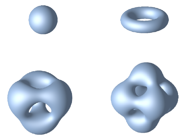
Figure 1: Energy density isosurfaces for the spherical 1-monopole, axial 2-monopole, tetrahedral 3-monopole and octahedral 5-monopole. These surfaces are shown in the ball model of $\hbox{\mybb H}^{3}$.

3.2 Axial 2-monopole

Taking $\xi_{m}=e^{2\pi im/3}$, with $m=0,1,2$ and writing $\rho^{2}=X_{1}^{2}+X_{2}^{2}$ yields

$$|\Phi|^{2}={\frac{{R}^{2}\left(1+{R}^{2}\right)^{2}-{\rho}^{2}\left(1+{R}^{4}\right)+\frac{1}{4}\,{\rho}^{4}}{\left(\left(1+{R}^{2}\right)^{2}-{\rho}^{2}\right)^{2}}}\,,$$ (3.8)

with energy density

$${\cal E}={\frac{\left(1-{R}^{2}\right)^{4}\bigl{(}\left(1+{R}^{2}\right)^{4}+22{\rho}^{2}\left(1+{R}^{2}\right)^{2}+4{\rho}^{4}\bigr{)}}{2\left(\left(1+{R}^{2}\right)^{2}-{\rho}^{2}\right)^{4}}}\,.$$ (3.9)

The poles in this case are on the equator of the 2-sphere, located at the vertices of an equilateral triangle. This is a triangle that can be rigidly rotated around the equator, producing only a gauge transformation, so the JNR instanton and the hyperbolic monopole to which it gives rise have axial symmetry. An energy density isosurface is shown in Figure 1.

3.3 Tetrahedral 3-monopole

The vertex Klein polynomial of the tetrahedron is ${\cal T}_{v}=\xi^{4}+2\sqrt{3}i\xi^{2}+1$, with the four roots $\pm(1+i)/(\sqrt{3}+1),\ \pm(1-i)/(\sqrt{3}-1)$. Using the JNR ansatz with these points $\xi_{m}$ as poles gives a tetrahedrally symmetric monopole of charge 3.

The Higgs field and energy density are best expressed, as before, in terms of the Cartesian coordinates $X_{1},X_{2},X_{3}$. The ring of tetrahedrally invariant homogeneous polynomials is generated by the polynomials of degrees two, three and four,

$$t_{2}=X_{1}^{2}+X_{2}^{2}+X_{3}^{2}\,,\quad t_{3}=X_{1}X_{2}X_{3}\,,\quad t_{4}=X_{1}^{4}+X_{2}^{4}+X_{3}^{4}\,.$$ (3.10)

The squared magnitude of the Higgs field can be expressed in terms of these. Explicitly, it is found that

$$|\Phi|^{2}=q_{1}/q_{2}\quad\mbox{where}$$ (3.11)

$$q_{1} =9t_{2}+216\sqrt{3}t_{3}+132t_{2}^{2}-24t_{4}-24\sqrt{3}t_{3}t_{2}+294t_{2}^{3}+48t_{4}t_{2}+192t_{3}^{2}-24\sqrt{3}t_{3}t_{2}^{2}$$

$$+132t_{2}^{4}-24t_{4}t_{2}^{2}+216\sqrt{3}t_{3}t_{2}^{3}+9t_{2}^{5}\,,$$

$$q_{2} =(9+15t_{2}+16\sqrt{3}t_{3}+15t_{2}^{2}+9t_{2}^{3})^{2}\,.$$

The zeros of the Higgs field have tetrahedral symmetry, and for the tetrahedrally symmetric 3-monopole in Euclidean space, it was found (partly numerically) that there are four zeros of multiplicity $1$ forming a tetrahedron, together with one anti-zero at the centre [8]. The same occurs for the hyperbolic monopole. Along the line $X_{1}=X_{2}=X_{3}=l/\sqrt{3}$, which passes through a vertex of the tetrahedron of poles, the above expression simplifies to

$$|\Phi|^{2}={\frac{{l}^{2}\left(3{l}^{2}+14l+3\right)^{2}}{\left(3{l}^{2}+4l+3\right)^{2}\left(3{l}^{2}-2l+3\right)^{2}}}\,,$$ (3.12)

which has zeros at $l=0$ and $l=(2\sqrt{10}-7)/3$, confirming the extra anti-zero of the Higgs field.

The energy density can be computed by applying the Laplace–Beltrami operator, but the result is complicated. It is used to obtain the energy density isosurface shown in Figure 1. Along the special line the energy density simplifies to

$${\cal E}=\frac{81(1-l^{2})^{4}\bigl{(}27(l^{8}+1)+72l(l^{6}+1)+1140l^{2}(l^{4}+1)+760l^{3}(l^{2}+1)+2402l^{4}\bigr{)}}{2(3l^{2}+4l+3)^{4}\,(3l^{2}-2l+3)^{4}}\,.$$ (3.13)

This expression is plotted in Figure 2.

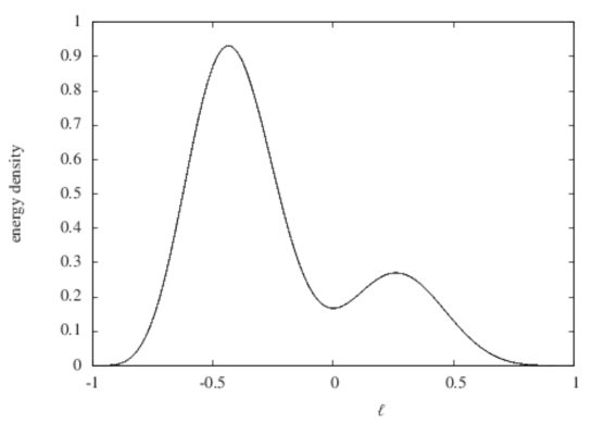
Figure 2: The energy density of the tetrahedral 3-monopole along a line through the origin and a vertex.

3.4 Octahedral 5-monopole

The JNR ansatz with six poles at the vertices of an octahedron gives a hyperbolic 5-monopole with octahedral symmetry. The vertex Klein polynomial of the octahedron is ${\cal O}_{v}=\xi^{5}-\xi$, with roots $\infty,\pm 1,\pm i,0$. The fact that one root is at infinity means that the JNR ansatz reduces to the ’t Hooft ansatz for an instanton [33, 21], where the first term in $\zeta$ is replaced by $1$.

The ring of octahedrally invariant homogeneous polynomials is generated by $o_{2}=t_{2},\,o_{4}=t_{4}$ and $o_{6}=t_{3}^{2}$, with $t_{2},t_{3}$ and $t_{4}$ as in (3.10). $|\Phi|^{2}$ can be written in terms of these invariants as

$$|\Phi|^{2}=q_{1}/q_{2}\quad\mbox{where}$$ (3.14)

$$q_{1} =o_{2}-32o_{4}+24o_{2}^{2}+76o_{2}^{3}+192o_{6}-80o_{4}o_{2}-32o_{4}o_{2}^{2}+104o_{2}^{4}-384o_{6}o_{2}^{2}+64o_{4}^{2}o_{2}$$

$$-96o_{4}o_{2}^{3}+166o_{2}^{5}-32o_{4}o_{2}^{4}+104o_{2}^{6}-80o_{4}o_{2}^{5}+76o_{2}^{7}+192o_{6}o_{2}^{4}-32o_{4}o_{2}^{6}+24o_{2}^{8}+o_{2}^{9}\,,$$

$$q_{2} =(3+4o_{2}-8o_{4}+10o_{2}^{2}+4o_{2}^{3}+3o_{2}^{4})^{2}(1+o_{2})^{2}\,.$$

An energy density isosurface is shown in Figure 1.

Along the $X_{3}$-axis (which passes through two vertices) the above simplifies to

$$|\Phi|^{2}={\frac{X_{3}^{2}\left(X_{3}^{2}+2X_{3}-1\right)^{2}\left(X_{3}^{2}-2X_{3}-1\right)^{2}}{\left(3X_{3}^{4}-2X_{3}^{2}+3\right)^{2}\left(X_{3}^{2}+1\right)^{2}}}\,,$$ (3.15)

which has zeros at $X_{3}=0$ and $X_{3}=\pm(\sqrt{2}-1)$. This is compatible with there being six zeros of multiplicity $1$ forming an octahedron, and an anti-zero at the centre, as in flat space [7].

Along this same axis,

$${\cal E}=\frac{(1-X_{3}^{2})^{4}\bigl{(}27(X_{3}^{16}+1)+120X_{3}^{2}(X_{3}^{12}+1)+5812X_{3}^{4}(X_{3}^{8}+1)+14408X_{3}^{6}(X_{3}^{4}+1)+21474X_{3}^{8}\bigr{)}}{2(X_{3}^{2}+1)^{4}\,(3X_{3}^{4}-2X_{3}^{2}+3)^{4}}\,,$$ (3.16)

and this is shown graphically in Figure 3.

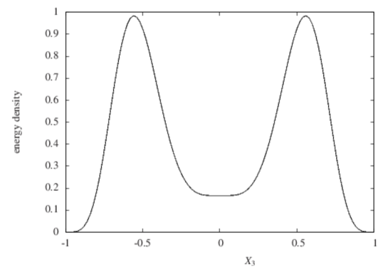
Figure 3: The energy density of the octahedral 5-monopole along the $X_{3}$-axis.

3.5 Icosahedral 11-monopole

The JNR ansatz with twelve poles at the vertices of an icosahedron gives a hyperbolic 11-monopole with icosahedral symmetry. In an orientation that has a root at infinity, the vertex Klein polynomial of the icosahedron is ${\cal Y}_{v}=\xi^{11}+11\xi^{6}-\xi.$

At charge 11 and higher, it becomes impractical to calculate explicit expressions for the magnitude of the Higgs field throughout hyperbolic space, due to the number of terms. However, the Higgs field of the icosahedral 11-monopole is manageable if restricted to the $X_{3}$-axis, and here

$$|\Phi|^{2}={\frac{X_{3}^{2}\left(25X_{3}^{8}+20X_{3}^{6}-218X_{3}^{4}+20X_{3}^{2}+25\right)^{2}}{\left(75X_{3}^{10}+55X_{3}^{8}-2X_{3}^{6}-2X_{3}^{4}+55X_{3}^{2}+75\right)^{2}}}\,.$$ (3.17)

Along this axis, which passes through two vertices, there are Higgs zeros at $X_{3}=0$ and $X_{3}^{2}=(2\sqrt{17}-1-2\sqrt{11-\sqrt{17}}\,)/5,$ compatible with twelve zeros of multiplicity 1 at the vertices of the icosahedron and an anti-zero at the centre.

4 Circle invariance of ADHM data

The JNR ansatz could be used to construct further hyperbolic monopoles, mostly with lower symmetry, by having the poles at more generic positions on the boundary surface of $\hbox{\mybb H}^{3}$, and changing the weights. However, one cannot obtain all hyperbolic monopoles this way. The dimension of the moduli space of hyperbolic monopoles of charge $N$ grows like $4N$, whereas that of the JNR parameter space (with poles restricted to a two-dimensional surface) grows like $3N$. The way to obtain all instantons in $\hbox{\mybb R}^{4}$ is to use the ADHM construction, and in this way one can also obtain all hyperbolic monopoles.

In this section we discuss the general class of ADHM data that give rise to hyperbolic monopoles. That means focussing on circle invariance first, leaving the possibility of platonic symmetry to later. We will use the toroidal coordinate system in $\hbox{\mybb R}^{4}$ which leads to the ball model of $\hbox{\mybb H}^{3}$. The ADHM matrices need to satisfy a number of simultaneous quadratic constraints, and these are not generally explicitly solvable.

The ADHM matrices are constant matrices of quaternions, and one also needs to use the quaternionic representation of a point $x$ in $\hbox{\mybb R}^{4}$, $x=x_{4}+x_{1}i+x_{2}j+x_{3}k$. Then the conformal group of $\hbox{\mybb R}^{4}$ acts as quaternionic Möbius transformations

$$x\mapsto x^{\prime}=(Ax+B)(Cx+D)^{-1}\,.$$ (4.1)

Platonic ADHM data are symmetric under some finite subgroup $K$ of $SO(3)$ generated by rotations of the form

$$\begin{pmatrix}A&B\\ C&D\end{pmatrix}=\begin{pmatrix}q&0\\ 0&q\end{pmatrix}\,,$$ (4.2)

where $q$ is a unit quaternion representing (in $SU(2)$) an element of $K$. The commuting circle action is given by the group of rotations

$$\begin{pmatrix}A&B\\ C&D\end{pmatrix}=\begin{pmatrix}\cos\frac{\alpha}{2}&\sin\frac{\alpha}{2}\\ -\sin\frac{\alpha}{2}&\cos\frac{\alpha}{2}\end{pmatrix}\,.$$ (4.3)

Note that this circle action fixes the 2-sphere given by $x$ a unit pure quaternion. This becomes the 2-sphere boundary of $\hbox{\mybb H}^{3}$ in the ball model.

In terms of the coordinates $X_{1},X_{2},X_{3}$ in the ball model, define the pure quaternion $X=X_{1}i+X_{2}j+X_{3}k$, with $R^{2}=|X|^{2}$. Together with the coordinate $\chi$ along the circle one obtains the toroidal coordinates of $\hbox{\mybb R}^{4}$. The corresponding expression for the quaternion $x$ is

$$x=\frac{2X+(1-R^{2})\sin\chi}{1+R^{2}+(1-R^{2})\cos\chi}\,.$$ (4.4)

The circle action (4.3) corresponds to the rotation $\chi\mapsto\chi+\alpha$.

In standard form, the ADHM data for a charge $N$ instanton are a pair of quaternionic matrices $L$ and $M$, where $L$ is a row of $N$ quaternions and $M$ is a symmetric $N\times N$ matrix of quaternions [16]. These are combined into

$$\widehat{M}=\begin{pmatrix}L\\ M\end{pmatrix}$$ (4.5)

and are required to satisfy the quadratic constraints

$$\widehat{M}^{\dagger}\,\widehat{M}=R_{N}\,,$$ (4.6)

where $R_{N}$ is an invertible, real $N\times N$ matrix. The pure quaternion part of $\widehat{M}^{\dagger}\,\widehat{M}$ is required to vanish. From $\widehat{M}$ one constructs the ADHM operator

$$\Delta(x)=\widehat{M}-Ux=\begin{pmatrix}L\\ M\end{pmatrix}-\begin{pmatrix}0\\ 1_{N}\end{pmatrix}x\,,$$ (4.7)

where $1_{N}$ denotes the $N\times N$ unit matrix.

Equivalent ADHM data are obtained by applying the transformation

$$\widehat{M}\mapsto Q\widehat{M}\,,\quad U\mapsto QU\,,$$ (4.8)

where $Q^{\dagger}Q=1_{N+1}$, but then the data are (generically) no longer in standard form.

We now introduce a stronger set of constraints on the ADHM data than (4.6), and show that these are sufficient for the data to be invariant under the circle action (4.3). The stronger constraints are

$$(i) M\mbox{\ is pure quaternion and symmetric,}$$ (4.9)

$$(ii) \widehat{M}^{\dagger}\,\widehat{M}=1_{N}\,,$$ (4.10)

$$(iii) LM=\mu L\,,\mbox{\ where $\mu$ is a pure quaternion, and $L$ is non-vanishing.}$$ (4.11)

We refer to $\mu$ as a left-eigenvalue of $M$. Properties $(i)$ and $(ii)$ imply that

$$L^{\dagger}L=1_{N}+M^{2}\,.$$ (4.12)

Another useful relation is

$$LL^{\dagger}=1-|\mu|^{2}\,.$$ (4.13)

To verify this, apply $M$ on the right of $(iii)$ to obtain $LM^{2}=\mu LM=\mu^{2}L=-|\mu|^{2}L$, where property $(iii)$ has been used again. Eliminating $M^{2}$ using (4.12) gives $(LL^{\dagger}-1+|\mu|^{2})L=0$, and the result follows.

Under the general conformal transformation (4.1) the ADHM data transform (up to an overall factor on the right) as

$$U\mapsto U^{\prime}=UA-\widehat{M}C\,,\ \quad\widehat{M}\mapsto\widehat{M}^{\prime}=\widehat{M}D-UB\,,$$ (4.14)

which are also not in standard form. For the case of the circle action (4.3) the transformation (4.14) becomes

$$U^{\prime}=U\cos\frac{\alpha}{2}+\widehat{M}\sin\frac{\alpha}{2}\,,\ \quad\widehat{M}^{\prime}=\widehat{M}\cos\frac{\alpha}{2}-U\sin\frac{\alpha}{2}\,.$$ (4.15)

To show that the constrained ADHM data are circle-invariant we need a matrix $Q$ to put these data back into standard form. Using constraints $(i)$ to $(iii)$ and the relations (4.12) and (4.13), one finds that the required matrix is

$$Q=\begin{pmatrix}\cos\frac{\alpha}{2}+\mu\sin\frac{\alpha}{2}&-L\sin\frac{\alpha}{2}\\ L^{\dagger}\sin\frac{\alpha}{2}&1_{N}\cos\frac{\alpha}{2}-M\sin\frac{\alpha}{2}\end{pmatrix}\,.$$ (4.16)

It can be checked that $Q^{\dagger}Q=1_{N+1}$, and direct calculation shows that $QU^{\prime}=U$ and $Q\widehat{M}^{\prime}=\widehat{M}$, so the ADHM data have the required circle invariance, and hence give rise to a hyperbolic monopole.

To proceed with the ADHM construction of the instanton, and hence monopole, we need to find an $(N+1)$-component column vector $\Psi$ of unit length, $\Psi^{\dagger}\Psi=1$, that solves the linear equation

$$\Psi^{\dagger}\Delta(x)=0\,.$$ (4.17)

Note that $\Psi$ is unaffected if $\Delta(x)$ is multiplied by a factor on the right. The instanton gauge potential is then obtained from the formula

$$A_{\mu}=\Psi^{\dagger}\partial_{\mu}\Psi\,,$$ (4.18)

where this pure quaternion is regarded as an element of $su(2)$.

Eq.(4.4) shows that when $\chi=0$, then $x=X$. Hence for circle-invariant data, and setting $\alpha=\chi$, we deduce that at a point $x$ with toroidal coordinates $X$ and $\chi$,

$$\Delta(x)=Q^{\dagger}\Delta(X)\,.$$ (4.19)

Here $Q$ is as in (4.16), with $\alpha=\chi$. The required vector $\Psi$ can therefore be written in the form $\Psi=Q^{\dagger}V$ where $V$ is a unit length column vector, $V^{\dagger}V=1$, that depends only on the pure quaternion $X$ and solves the linear equation

$$V^{\dagger}\Delta(X)=0\,.$$ (4.20)

The resulting gauge potential is $\chi$-independent, which is what we need to interpret the instanton as a hyperbolic monopole. In particular, the Higgs field of the monopole is

$$\Phi=A_{\chi}=V^{\dagger}\,\Xi\,V\,,$$ (4.21)

where

$$\Xi=Q\,\partial_{\chi}Q^{\dagger}=\frac{1}{2}\begin{pmatrix}-\mu&L\\ -L^{\dagger}&M\end{pmatrix}\,.$$ (4.22)

Interestingly, the left-eigenvalue $\mu$ has a physical meaning, in that it is related to the value of the Higgs field at the origin. To see this, set $X=0$ and observe that at this point the vector $V$ satisfying (4.20) is simply

$$V=\begin{pmatrix}\mu\\ L^{\dagger}\end{pmatrix}\,.$$ (4.23)

Substituting this into the expression (4.21) yields $\Phi(0)=-\frac{1}{2}\mu$. The gauge invariant quantity is $|\Phi(0)|=\frac{1}{2}|\mu|$.

As mentioned earlier, Braam and Austin have previously discussed hyperbolic monopoles in terms of ADHM data invariant under a circle action [27]. Their analysis is for all half-integer $p$ and their approach used the circle action on $\hbox{\mybb R}^{4}$ that leads to the upper half space version of $\hbox{\mybb H}^{3}$. Our analysis, adapted to the hyperbolic ball, is more restricted and only deals with the case $p=\frac{1}{2}$. Its advantage is that we will be able to explicitly find hyperbolic monopoles with platonic symmetry. To make a connection to the work of Braam and Austin would require proving a correspondence between ADHM data that satisfies our constraints $(i)$ to $(iii)$ and ADHM data with complex entries. This would also clarify the issue of whether or not our sufficient constraints are also necessary, which at the moment is unknown.

5 Hyperbolic monopoles from ADHM data

In this section we give explicit examples of ADHM data satisfying the constraints $(i)$ to $(iii)$ discussed in Section 4, and which therefore give rise to hyperbolic monopoles. Many have platonic symmetry. Some of the examples reproduce results obtained using the JNR ansatz.

For $N=1$ and $N=2$ we can directly find ADHM data satisfying the constraints. For larger $N$, we make use of ADHM matrices that were previously constructed to give platonically symmetric instantons [25, 26, 34]. These can be written down explicitly, after some analysis involving the representation theory of the relevant platonic symmetry group, $K$. They are seen to satisfy the constraints provided one fixes their normalisation suitably, which corresponds to fixing the scale of the instanton.

It was not recognised previously that these platonic instantons may have an additional circle invariance, and hence correspond to hyperbolic monopoles.

5.1 $N=1$

An admissible $\widehat{M}$, satisfying the constraints, is

$$\widehat{M}=\begin{pmatrix}\sqrt{1-a^{2}}\\ ai\end{pmatrix}\,,$$ (5.1)

with $|a|<1$ and $\mu=ai$. This gives a hyperbolic 1-monopole with its centre along the $X_{1}$-axis at $X_{1}=(1-\sqrt{1-a^{2}})/a$. The Higgs field at the origin has magnitude $|\Phi(0)|=\frac{1}{2}|\mu|=\frac{1}{2}|a|$. The squared magnitude of the Higgs field at a general point in the unit ball is given by

$$|\Phi|^{2}=\frac{4R^{2}-4aX_{1}(1+R^{2})+a^{2}(4X_{1}^{2}+(1-R^{2})^{2})}{4(1+R^{2}-2aX_{1})^{2}}.$$ (5.2)

The simplest example is

$$\widehat{M}=\begin{pmatrix}1\\ 0\end{pmatrix}\,,$$ (5.3)

with the monopole centred at the origin. The formulae (3.6) and (3.7) for the Higgs field magnitude and energy density are easily rederived.

All of these monopoles are spherically symmetric about their centres, but only in the last case is the symmetry group the standard $SO(3)$ that we have been discussing.

5.2 $N=2$

An axially symmetric 2-monopole, centred at the origin, is obtained from

$$\widehat{M}=\frac{1}{2}\begin{pmatrix}\sqrt{2}&\sqrt{2}k\\ i&j\\ j&-i\end{pmatrix}\,.$$ (5.4)

This can be extended to a one-parameter family of non-axially symmetric monopoles, still centred at the origin. This family illustrates the $90^{\circ}$ scattering of $N=2$ monopoles, familiar from monopoles in $\hbox{\mybb R}^{3}$ [20]. $\widehat{M}$ has the form, satisfying the constraints,

$$\widehat{M}=\frac{1}{2}\begin{pmatrix}\sqrt{2(1-a^{2})}&\sqrt{2(1-a^{2})}k\\ (1-a)i&(1+a)j\\ (1+a)j&-(1-a)i\end{pmatrix}\,,$$ (5.5)

where $a\in(-1,1)$. The axial case is recovered when $a=0$. For this family, the left-eigenvalue of $M$ is $\mu=-ai$, so it vanishes only for the axial example.

$|\Phi|^{2}$ can be computed at all points in the unit ball, and is

$$|\Phi|^{2}=q_{1}/q_{2}\quad\mbox{where}$$ (5.6)

$$q_{1} =(a^{4}+1)\rho^{4}-2a^{3}(X_{1}^{2}-X_{2}^{2})((1-R^{2})^{2}+2\rho^{2})+a^{2}((1-R^{4})^{2}-8R^{2}\rho^{2}+6\rho^{4}-16X_{1}^{2}X_{2}^{2})$$

$$+2a(X_{1}^{2}-X_{2}^{2})(3R^{4}+2R^{2}+3-2\rho^{2})+4R^{2}(1+R^{2})^{2}-4\rho^{2}(1+R^{4})\,,$$

$$q_{2} =\bigl{(}-2a^{2}\rho^{2}+4a(X_{1}^{2}-X_{2}^{2})+2((1+R^{2})^{2}-\rho^{2})\bigr{)}^{2}\,,$$

and where $\rho^{2}=X_{1}^{2}+X_{2}^{2}$. Note that when $a=0$ this expression reverts to the axial form (3.8) obtained earlier using JNR data. The symmetry under a change of sign of $a$ accompanied by an exchange of $X_{1}$ and $X_{2}$ is clear.

For $a\in(-1,0]$ the two zeros of the Higgs field are on the $X_{1}$-axis at the positions

$$X_{1}^{2}=\frac{a^{2}-3+\sqrt{(1-a^{2})(9-a^{2})}}{2a}\,.$$ (5.7)

For $a\in[0,1)$ the Higgs zeros are on the $X_{2}$-axis, as expected from the above symmetry under $a\mapsto-a$. Energy density isosurfaces for several members of this one-parameter family are displayed in Figure 4.

Figure 4: Energy density isosurfaces for the 2-monopole with $a=-0.5,-0.25,0,0.25,0.5.$ The boundary of hyperbolic space is also indicated.

5.3 Tetrahedral $N=3$

The ADHM data with the normalisation required to satisfy the constraints are of the form [34]

$$\widehat{M}=\frac{1}{\sqrt{3}}\begin{pmatrix}i&j&k\\ 0&k&j\\ k&0&i\\ j&i&0\end{pmatrix}\,,$$ (5.8)

with $\mu=0$. From this one obtains the Higgs field and energy density of the tetrahedrally symmetric 3-monopole obtained earlier using JNR data.

5.4 Cubic $N=4$

This is the first platonic example that cannot be obtained using the JNR ansatz. Here

$$\widehat{M}=\frac{1}{2\sqrt{2}}\begin{pmatrix}\sqrt{2}&\sqrt{2}i&\sqrt{2}j&\sqrt{2}k\\ 0&-j-k&-k-i&-i-j\\ -j-k&0&j-i&i-k\\ -k-i&j-i&0&k-j\\ -i-j&i-k&k-j&0\end{pmatrix}\,.$$ (5.9)

This is a special case of the ADHM data found in [25], with the normalisation, and hence the instanton scale size, fixed to satisfy the constraints. The hyperbolic monopole has

$$|\Phi|^{2}=q_{1}/q_{2}\quad\mbox{where}$$ (5.10)

$$q_{1} =-18o_{2}^{2}+54o_{4}+54o_{2}^{3}+108o_{6}+18o_{4}o_{2}+153o_{2}^{4}-216o_{6}o_{2}+9o_{4}^{2}-54o_{4}o_{2}^{2}+18o_{4}o_{2}^{3}$$

$$+54o_{2}^{5}+108o_{6}o_{2}^{2}+54o_{4}o_{2}^{4}-18o_{2}^{6}\,,$$

$$q_{2} =4(2o_{2}^{4}+4o_{2}^{3}+3o_{2}^{2}+3o_{4}+4o_{2}+2)^{2}\,,$$

with $o_{2},o_{4}$ and $o_{6}$ the octahedral polynomials as in (3.14). Along the line $X_{1}=X_{2}=X_{3}=l/\sqrt{3}$ (which passes through two cubic vertices) the above simplifies to

$$|\Phi|^{2}=\frac{4l^{6}}{(l^{2}+1)^{2}(l^{4}+1)^{2}}\,.$$ (5.11)

This is zero only at the origin, in agreement with the fact that for the cubically symmetric 4-monopole in $\hbox{\mybb R}^{3}$ there are no anti-zeros of the Higgs field. Along this line the energy density is

$${\cal E}={\frac{{l}^{2}\left(9\,{l}^{12}+102\,{l}^{10}+283\,{l}^{8}+396\,{l}^{6}+283\,{l}^{4}+102\,{l}^{2}+9\right)\left(1-l^{2}\right)^{4}}{2\left({l}^{4}+1\right)^{4}\left({l}^{2}+1\right)^{4}}}\,.$$ (5.12)

An energy density isosurface for the cubic 4-monopole is presented in Figure 5.

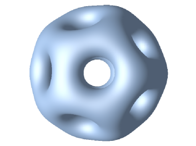
Figure 5: Energy density isosurfaces for the cubic 4-monopole and the dodecahedral 7-monopole.

The cubically symmetric data can be extended to a one-parameter family with tetrahedral symmetry, as in [25],

$$\widehat{M}=\left(\begin{array}[]{cccc}b\sqrt{2}&b\sqrt{2}i&b\sqrt{2}j&b\sqrt{2}k\\ \vskip 6.0pt plus 2.0pt minus 2.0pt\cr a\left(i+j+k\right)&-b\left(j+k\right)&-b\left(k+i\right)&-b\left(i+j\right)\\ \vskip 6.0pt plus 2.0pt minus 2.0pt\cr-b\left(j+k\right)&a\left(i-j-k\right)&b\left(j-i\right)&b\left(i-k\right)\\ \vskip 6.0pt plus 2.0pt minus 2.0pt\cr-b\left(k+i\right)&b\left(j-i\right)&a\left(-i+j-k\right)&b\left(k-j\right)\\ \vskip 6.0pt plus 2.0pt minus 2.0pt\cr-b\left(i+j\right)&b\left(i-k\right)&b\left(k-j\right)&a\left(-i-j+k\right)\end{array}\right)\,,$$ (5.13)

where, to satisfy the constraints, $b=\sqrt{(1-3a^{2})/8}$ with $\sqrt{3}a\in(-1,1)$. The cubic case is recovered when $a=0$ and $b=1/2\sqrt{2}$. For this tetrahedral family it can be checked that the left-eigenvalue is $\mu=a(i+j+k)$, so it vanishes only for the cubic example. Energy density isosurfaces for several members of this one-parameter family are displayed in Figure 6.

Figure 6: Energy density isosurfaces for the 4-monopole with $a=-0.4\,,-0.2\,,0\,,0.2\,,0.4\,.$ The boundary of hyperbolic space is also indicated.

5.5 Dodecahedral $N=7$

The existence of icosahedrally symmetric ADHM data with $N=7$ was established in [26]. With a suitable normalisation, the data satisfy the constraints $(i)$ to $(iii)$, with $\mu=0$, and give a hyperbolic 7-monopole of dodecahedral form. $\widehat{M}$ is

$$\widehat{M}=\frac{1}{2}\begin{pmatrix}1&i&j&k&0&0&0\\ 0&0&0&0&i&j&k\\ 0&0&0&0&0&\tau k&\tau^{-1}j\\ 0&0&0&0&\tau^{-1}k&0&\tau i\\ 0&0&0&0&\tau j&\tau^{-1}i&0\\ i&0&\tau^{-1}k&\tau j&0&0&0\\ j&\tau k&0&\tau^{-1}i&0&0&0\\ k&\tau^{-1}j&\tau i&0&0&0&0\\ \end{pmatrix}\,,$$ (5.14)

where $\tau=\frac{1}{2}(\sqrt{5}+1)$.

The ring of icosahedrally invariant homogeneous polynomials is generated by three polyomials of degrees two, six and ten,

$$y_{2} = X_{1}^{2}+X_{2}^{2}+X_{3}^{2}\,,$$ (5.15)

$$y_{6} = 2\tau(X_{1}^{4}X_{2}^{2}+X_{2}^{4}X_{3}^{2}+X_{3}^{4}X_{1}^{2})-2\tau^{-1}(X_{1}^{4}X_{3}^{2}+X_{2}^{4}X_{1}^{2}+X_{3}^{4}X_{2}^{2})-8X_{1}^{2}X_{2}^{2}X_{3}^{2}\,,$$

$$y_{10} = 10X_{1}^{2}X_{2}^{2}X_{3}^{2}\left(5X_{1}^{2}X_{2}^{2}+5X_{1}^{2}X_{3}^{2}+5X_{2}^{2}X_{3}^{2}-2X_{1}^{4}-2X_{2}^{4}-2X_{3}^{4}\right)$$

$$+2\sqrt{5}\bigl{(}X_{1}^{2}X_{2}^{8}-X_{2}^{2}X_{1}^{8}+X_{1}^{8}X_{3}^{2}-X_{3}^{8}X_{1}^{2}+X_{3}^{8}X_{2}^{2}-X_{2}^{8}X_{3}^{2}$$

$$-{\tau}\left(X_{1}^{4}X_{2}^{6}+X_{2}^{4}X_{3}^{6}+X_{3}^{4}X_{1}^{6}\right)-{\tau^{-1}}\left(X_{1}^{4}X_{3}^{6}+X_{2}^{4}X_{1}^{6}+X_{3}^{4}X_{2}^{6}\right)\bigr{)}\,.$$

The squared magnitude of the Higgs field can be expressed in terms of these, and is

$$|\Phi|^{2}=q_{1}/q_{2}\quad\mbox{where}$$ (5.16)

$$q_{1} =8y_{2}^{3}+60y_{6}+56y_{2}^{4}+180y_{6}y_{2}+194y_{2}^{5}+185y_{6}y_{2}^{2}+25y_{10}+392y_{2}^{6}-20y_{6}y_{2}^{3}$$

$$+500y_{2}^{7}-50y_{10}y_{2}^{2}+50y_{6}^{2}y_{2}-210y_{6}y_{2}^{4}+392y_{2}^{8}-20y_{6}y_{2}^{5}+194y_{2}^{9}+25y_{10}y_{2}^{4}$$

$$+185y_{6}y_{2}^{6}+56y_{2}^{10}+180y_{6}y_{2}^{7}+8y_{2}^{11}+60y_{6}y_{2}^{8}\,,$$

$$q_{2} =2(1+y_{2})^{2}(2+4y_{2}+6y_{2}^{2}+6y_{2}^{3}+5y_{6}+6y_{2}^{4}+4y_{2}^{5}+2y_{2}^{6})^{2}\,.$$

An energy density isosurface for the dodecahedral 7-monopole is presented in Figure 5.

5.6 Icosahedral $N=17$

Icosahedrally symmetric ADHM data for an instanton with $N=17$ are given in [35]. In this example the matrix $\widehat{M}$ is quite large, so we do not reproduce it here. However it can be checked that it does indeed satisfy the constraints $(i)$ to $(iii)$ for circle invariance, after multiplication by a scale factor of $\frac{1}{2}$ compared to the normalisation presented in [35]. The left-eigenvalue $\mu$ again vanishes. Although we have not attempted to compute the Higgs field and energy density of the resulting 17-monopole, the known properties of the instanton make it clear that the polyhedron associated with this example is the truncated icosahedron, familiar as the buckyball.

6 Rational maps

One of the achievements of earlier work on hyperbolic monopoles [10, 27] was the establishment of a one-to-one correspondence between charge $N$ monopoles and rational maps (from the Riemann sphere to itself) of degree $N$.

We have not succeeded in constructing a rational map from a general hyperbolic monopole, in our formalism. However in the cases where $\mu=0$ we have a good candidate. This appears to be an analogue of the Jarvis map for Euclidean monopoles [28]. In particular, the map has platonic symmetry if the monopole has platonic symmetry.

To proceed, let $X$ be a unit pure quaternion. This can be identified with a point on the Riemann sphere with complex coordinate $\xi$ by writing

$$X=\frac{1}{1+|\xi|^{2}}\bigg{(}2\,{\rm Re}(\xi)i+2\,{\rm Im}(\xi)j+(|\xi|^{2}-1)k\bigg{)}\,.$$ (6.1)

Next, use the ADHM data to define the quaternion function of $X$,

$$f(X)=L(M-X)^{-1}L^{\dagger}\,,$$ (6.2)

where $M-X$ means $M-X\,1_{N}$. Using constraint $(i)$, it is easy to see that $f$ is a pure quaternion for all $X$.

If $\mu=0$, then $|f|^{2}=1$ so $f$ is a unit pure quaternion. To prove this, note first that as $f$ is a pure quaternion,

$$|f|^{2}=-L(M-X)^{-1}L^{\dagger}L(M-X)^{-1}L^{\dagger}$$ (6.3)

and therefore, using (4.12),

$$|f|^{2}=-L(M-X)^{-1}(1_{N}+M^{2})(M-X)^{-1}L^{\dagger}\,.$$ (6.4)

Next, as $X$ is a unit pure quaternion, $(M-X)^{-1}=(-X(1_{N}+XM))^{-1}=(1_{N}+XM)^{-1}X$, from which follows the formal series expansion

$$(M-X)^{-1}=X-XMX+XMXMX-XMXMXMX+\cdots\,.$$ (6.5)

Inserting this twice in (6.4), using $X^{2}=-1$, and collecting terms, we obtain the relatively simple series

$$|f|^{2}=-L(-1_{N}+MX+XM-MXMX-XMXM+MXMXMX+XMXMXM-\cdots)L^{\dagger}\,.$$ (6.6)

If $\mu=0$, then $LM=0$, using constraint $(iii)$, and by conjugation $ML^{\dagger}=0$, so all terms in this series except the first vanish, and by (4.13), $LL^{\dagger}=1$, so $|f|^{2}=1$, as claimed.

The unit pure quaternion $f$, like $X$, may be identified with a Riemann sphere coordinate ${\cal R}$ via

$$f=\frac{1}{1+|{\cal R}|^{2}}\bigg{(}2\,{\rm Re}({\cal R})i+2\,{\rm Im}({\cal R})j+(|{\cal R}|^{2}-1)k\bigg{)}\,.$$ (6.7)

The function $f(X)$ therefore gives a function ${\cal R}(\xi)$, our candidate rational map, although at this point ${\cal R}$ could also depend on $\bar{\xi}$.

To prove that ${\cal R}(\xi)$ is holomorphic, we recall the complex structure on the Riemann sphere of unit pure quaternions. Let $X+\delta X$ be a unit pure quaternion infinitesimally separated from $X$. Since $X^{2}=-1$ and $(X+\delta X)^{2}=-1$, to linear order $X\delta X+\delta XX=0$. This is the condition for $\delta X$ to be tangent to the Riemann sphere at $X$. The complex structure operation at $X$ is right multiplication by $X$, $\delta X\to\delta XX$, which acts on the tangent space and whose square is multiplication by $-1$. Similarly, the complex structure on the target Riemann sphere is right multiplication by $f$.

Now consider $\delta f$, effectively the derivative of $f(X)$, defined as $f(X+\delta X)-f(X)$ truncated at linear order in $\delta X$. From (6.2), we find

$$\delta f=L(M-X)^{-1}\delta X(M-X)^{-1}L^{\dagger}\,.$$ (6.8)

${\cal R}(\xi)$ will be holomorphic if the effect of replacing $\delta X$ by $\delta XX$ is to replace $\delta f$ by $\delta ff$. So we need to show that

$$L(M-X)^{-1}\delta XX(M-X)^{-1}L^{\dagger}=L(M-X)^{-1}\delta X(M-X)^{-1}L^{\dagger}L(M-X)^{-1}L^{\dagger}\,.$$ (6.9)

The first few factors on each side are the same, so it is sufficient to show that

$$X(M-X)^{-1}L^{\dagger}=(M-X)^{-1}L^{\dagger}L(M-X)^{-1}L^{\dagger}\,.$$ (6.10)

Using the series (6.5) again, and the relations (4.12) and $X^{2}=-1$, this reduces to

$$(-1_{N}+MX-MXMX+\cdots)L^{\dagger}=(-1_{N}+MX+XM-MXMX-XMXM+\cdots)L^{\dagger}\,.$$ (6.11)

As $ML^{\dagger}=0$, the left and right hand sides are equal, so ${\cal R}(\xi)$ is indeed holomorphic.

In fact, for all our platonic monopole examples with $\mu=0$, we find that ${\cal R}$ is a rational function of $\xi$ whose degree equals the monopole charge. In detail, for the spherical 1-monopole and the axial 2-monopole the maps are ${\cal R}=\xi$ and ${\cal R}=\xi^{2}$, respectively. More complicated examples are provided by the tetrahedral 3-monopole and the dodecahedral 7-monopole, where the above construction yields the rational maps

$${\cal R}=\frac{\sqrt{3}i\xi^{2}-1}{\xi^{3}-\sqrt{3}i\xi}\quad\quad\mbox{and}\quad\quad{\cal R}=\frac{7\xi^{6}-7\sqrt{5}\xi^{4}-7\xi^{2}-\sqrt{5}}{\sqrt{5}\xi^{7}+7\xi^{5}+7\sqrt{5}\xi^{3}-7\xi}\,.$$ (6.12)

These maps agree with the Jarvis maps presented in [36] for the corresponding platonic monopoles in Euclidean space.

7 Beyond $p=\frac{1}{2}$

The JNR construction of hyperbolic monopoles, presented in Section 3, applies only to the case $p=\frac{1}{2}.$ To obtain hyperbolic monopoles with other half-integer values of $p$ requires a placement of the poles out of the plane $r=0.$ However, once the poles do not lie in this fixed set of the circle action then it is more difficult to arrange for circle invariance. In fact the poles must all have the same weight and be equally spaced on a circle. This arrangement was first identified by Nash [19], who noted that the 1-monopole is obtained from a JNR instanton of charge $2p$ by placing equal weight poles at the vertices of a regular $(2p+1)$-gon inscribed in the circle $r=1$ with $x_{1}=x_{2}=0.$ Note that the case $p=\frac{1}{2}$ is again special here, in that this description of the 1-monopole involving two poles is equivalent to the earlier description, where two poles are placed in the $r=0$ plane. This dual description follows from the $SO(4)$ symmetry of the 1-instanton.

For $p\neq\frac{1}{2}$ the above polygonal arrangement is the only option for circle invariance, so more complicated monopoles with platonic symmetry are beyond this JNR ansatz. The ADHM construction, or its circle-invariant formulation by Braam and Austin, is then required. The possibility of an explicit construction of platonic monopoles is therefore not guaranteed, and certainly requires a full description of the non-standard action of $SO(3)$ on such data.

We now return to the discussion of circle-invariant ADHM data, as described in Section 4, and make some comments regarding its extension beyond $p=\frac{1}{2}.$ First of all, it is not apparent from the constraints $(i)$ to $(iii)$, that these apply to hyperbolic monopoles with $p=\frac{1}{2}.$ This is only evident upon examination of the associated compensating matrix (4.16), which reveals that it involves only the half-angle $\alpha/2,$ hence $p=\frac{1}{2}.$ To illustrate the challenges that arise in attempting to go beyond $p=\frac{1}{2}$ within this formalism, we present the construction of the 1-monopole with $p=1.$

Consider the 2-instanton given by the following ADHM data,

$$\widehat{M}=\frac{1}{\sqrt{3}}\begin{pmatrix}2\sqrt{2}&0\\ 0&1\\ 1&0\end{pmatrix}.$$ (7.1)

$\widehat{M}$ is obviously $SO(3)$ symmetric, as it contains only real entries and hence is invariant under rotations given by (4.2) for all unit quaternions $q.$ To show that this data is also circle-invariant, we need to demonstrate that the circle action (4.15) can be compensated. This requires that

$$QU^{\prime}P=U\quad\quad\mbox{and}\quad\quad Q\widehat{M}^{\prime}P=\widehat{M},$$ (7.2)

for some $3\times 3$ matrix $Q$ with $Q^{\dagger}Q=1_{3},$ and some invertible $2\times 2$ matrix $P.$ In the case that $p=\frac{1}{2},$ the corresponding transformation (4.8), mapping to equivalent ADHM data, did not explicitly include the matrix $P$ because it simplifies to the identity matrix. For $p\neq\frac{1}{2}$ this simplification is no longer possible.

It may be verified that the required matrices are given by

$$Q=\begin{pmatrix}\frac{1}{3}(1+2\cos\alpha)&-\sqrt{\frac{2}{3}}\sin\alpha&\frac{\sqrt{2}}{3}(1-\cos\alpha)\\ \sqrt{\frac{2}{3}}\sin\alpha&\cos\alpha&-\frac{1}{\sqrt{3}}\sin\alpha\\ \frac{\sqrt{2}}{3}(1-\cos\alpha)&\frac{1}{\sqrt{3}}\sin\alpha&\frac{1}{3}(2+\cos\alpha)\end{pmatrix}\quad\mbox{and}\quad P=\begin{pmatrix}\cos\frac{\alpha}{2}&\frac{1}{\sqrt{3}}\sin\frac{\alpha}{2}\\ -\sqrt{3}\sin\frac{\alpha}{2}&\cos\frac{\alpha}{2}\end{pmatrix}.$$ (7.3)

As before, the value of $p$ is not apparent in the ADHM data (7.1), but is evident in the compensating matrix $Q,$ which involves functions of the angle $p\alpha$ with $p=1.$ This contrasts with the $p=\frac{1}{2}$ compensating matrix (4.16), which involves functions of the half-angle $\frac{\alpha}{2}.$

The ADHM construction of the hyperbolic monopole proceeds as before by setting $\alpha=\chi$ so that

$$\Phi=A_{\chi}=V^{\dagger}\,\Xi\,V\,,$$ (7.4)

where

$$\Xi=Q\,\partial_{\chi}Q^{\dagger}=\frac{1}{\sqrt{3}}\begin{pmatrix}0&\sqrt{2}&0\\ -\sqrt{2}&0&1\\ 0&-1&0\end{pmatrix}$$ (7.5)

and $V$ is a unit length solution of (4.20). $\Xi$ has a different form to the $p=\frac{1}{2}$ expression (4.22). The corresponding magnitude of the Higgs field reproduces the $p=1$ spherically symmetric 1-monopole formula (2.18).

The $p=1$ ADHM data (7.1) does not satisfy any of our three constraints $(i)$ to $(iii)$ applicable to $p=\frac{1}{2}$ monopoles. For example,

$$\widehat{M}^{\dagger}\widehat{M}=\begin{pmatrix}3&0\\ 0&\frac{1}{3}\end{pmatrix}.$$ (7.6)

This demonstrates that our new constraints are specific to $p=\frac{1}{2}$ monopoles, and it is not known whether there is an appropriate generalisation to other half-integer values of $p.$

8 Conclusion

We have described methods to construct explicit examples of hyperbolic monopoles using circle-invariant instantons, both within the JNR and ADHM approaches. Several examples have been presented in detail, including a number with platonic symmetry. These solutions provide analytic information about hyperbolic monopoles that complements similar (though sometimes numerical) results known for monopoles in flat space.

The platonic examples discussed in this paper are singled out by their symmetry properties, but energetically they are simply points in a large moduli space of BPS hyperbolic monopoles. However, an additional motivation to study these symmetric examples is provided by the related problem for monopoles in four-dimensional Anti-de Sitter spacetime, which has three-dimensional hyperbolic space as its constant time slices. In the Anti-de Sitter case there is essentially a unique minimal energy monopole for each charge, rather than a moduli space, and numerical results [11] suggest that the minimal energy monopole is often of the symmetric type considered here. Analytic formulae in the hyperbolic case may therefore be useful in understanding the features of monopoles observed in the less tractable Anti-de Sitter situation.

There are many similarities between monopoles and Skyrmions [21], and this work provides the opportunity to investigate a new connection. It has been observed [13] that Skyrmions with massive pions may be approximated by Skyrmions with massless pions in hyperbolic space, which in turn can be approximated by the holonomy along circles of suitable instantons. If the instantons are taken to be circle-invariant, as in the present paper, then the computation of the holonomy involves no integration, and the result is an approximation of Skyrmions by the exponential of the Higgs field of a hyperbolic monopole, in a suitable gauge. The explicit hyperbolic monopoles presented in this paper will allow a detailed investigation of this issue.

References

- [1] R. S. Ward, Two Yang–Mills–Higgs monopoles close together, Phys. Lett. B102, 136 (1981).
- [2] P. Forgács, Z. Horváth and L. Palla, Exact multimonopole solutions in the Bogomolny–Prasad–Sommerfield limit, Phys. Lett. B99, 232 (1981); Solution-generating technique for self-dual monopoles, Nucl. Phys. B229, 77 (1983).
- [3] M. K. Prasad and P. Rossi, Construction of exact Yang–Mills–Higgs multimonopoles of arbitrary charge, Phys. Rev. Lett. 46, 806 (1981).
- [4] W. Nahm, The construction of all self-dual multimonopoles by the ADHM method, in Monopoles in Quantum Field Theory, eds. N. S. Craigie, P. Goddard and W. Nahm, Singapore, World Scientific, 1982.
- [5] N. J. Hitchin, On the construction of monopoles, Commun. Math. Phys. 89, 145 (1983).
- [6] N. J. Hitchin, N. S. Manton and M. K. Murray, Symmetric monopoles, Nonlinearity 8, 661 (1995).
- [7] C. J. Houghton and P. M. Sutcliffe, Octahedral and dodecahedral monopoles, Nonlinearity 9, 385 (1996).
- [8] C. J. Houghton and P. M. Sutcliffe, Tetrahedral and cubic monopoles, Commun. Math. Phys. 180, 343 (1996).
- [9] P. M. Sutcliffe, Monopole zeros, Phys. Lett. B376, 103 (1996).
- [10] M. F. Atiyah, Magnetic monopoles in hyperbolic spaces, in M. Atiyah: Collected Works, vol. 5, Oxford, Clarendon Press, 1988.
- [11] P. M. Sutcliffe, Monopoles in AdS, JHEP 1108, 032 (2011).
- [12] N. S. Manton and T. M. Samols, Skyrmions on and from instantons, J. Phys. A23, 3749 (1990).
- [13] M. F. Atiyah and P. M. Sutcliffe, Skyrmions, instantons, mass and curvature, Phys. Lett. B605, 106 (2005).
- [14] R. Jackiw, C. Nohl and C. Rebbi, Conformal properties of pseudoparticle configurations, Phys. Rev. D15, 1642 (1977).
- [15] E. Corrigan and D. B. Fairlie, Scalar field theory and exact solutions to a classical gauge theory, Phys. Lett. B67, 69 (1977).
- [16] M. F. Atiyah, N. J. Hitchin, V. G. Drinfeld and Yu. I. Manin, Construction of instantons, Phys. Lett. A65, 185 (1978).
- [17] A. Jaffe and C. Taubes, Vortices and Monopoles, Boston, Birkhäuser, 1980.
- [18] A. Chakrabarti, Construction of hyperbolic monopoles, J. Math. Phys. 27, 340 (1986).
- [19] C. Nash, Geometry of hyperbolic monopoles, J. Math. Phys. 27, 2160 (1986).
- [20] M. F. Atiyah and N. J. Hitchin, The Geometry and Dynamics of Magnetic Monopoles, Princeton University Press, 1988.
- [21] N. Manton and P. Sutcliffe, Topological Solitons, Cambridge University Press, 2004.
- [22] Ya. Shnir, Magnetic Monopoles, Berlin Heidelberg, Springer, 2005.
- [23] M. K. Prasad and C. M. Sommerfield, Exact classical solution for the ’t Hooft monopole and the Julia–Zee dyon, Phys. Rev. Lett. 35, 760 (1975).
- [24] E. B. Bogomolny, The stability of classical solutions, Sov. J. Nucl. Phys. 24, 449 (1976).
- [25] R. A. Leese and N. S. Manton, Stable instanton-generated Skyrme fields with baryon numbers three and four, Nucl. Phys. A572, 575 (1994).
- [26] M. A. Singer and P. M. Sutcliffe, Symmetric instantons and Skyrme fields, Nonlinearity 12, 987 (1999).
- [27] P. J. Braam and D. M. Austin, Boundary values of hyperbolic monopoles, Nonlinearity 3, 809 (1990).
- [28] S. Jarvis, A rational map for Euclidean monopoles via radial scattering, J. reine angew. Math. 524, 17 (2000).
- [29] M. K. Murray and M. A. Singer, Spectral curves of non-integral hyperbolic monopoles, Nonlinearity 9, 973 (1996); On the complete integrability of the discrete Nahm equations, Commun. Math. Phys. 210, 497 (2000).
- [30] P. Norbury and N. Romão, Spectral curves and the mass of hyperbolic monopoles, Commun. Math. Phys. 270, 295 (2007).
- [31] F. Klein, Lectures on the Icosahedron, London, Kegan Paul, 1913.
- [32] R. S. Ward, A Yang–Mills–Higgs monopole of charge 2, Commun. Math. Phys. 79, 317 (1981).
- [33] G. ’t Hooft, unpublished.
- [34] C. J. Houghton, Instanton vibrations of the 3-Skyrmion, Phys. Rev. D60, 105003 (1999).
- [35] P. M. Sutcliffe, Instantons and the buckyball, Proc. R. Soc. Lond. A460, 2903 (2004).
- [36] C. J. Houghton, N. S. Manton and P. M. Sutcliffe, Rational maps, monopoles and Skyrmions, Nucl. Phys. B510, 507 (1998).