Full density matrix numerical renormalization group calculation of impurity susceptibility and specific heat of the Anderson impurity model

Abstract

Recent developments in the numerical renormalization group (NRG) allow the construction of the full density matrix (FDM) of quantum impurity models (see A. Weichselbaum and J. von Delft in Ref. Weichselbaum and von Delft, 2007) by using the completeness of the eliminated states introduced by F.  B.  Anders and A.  Schiller in Ref. Anders and Schiller, 2005. While these developments prove particularly useful in the calculation of transient response and finite temperature Green’s functions of quantum impurity models, they may also be used to calculate thermodynamic properties. In this paper, we assess the FDM approach to thermodynamic properties by applying it to the Anderson impurity model. We compare the results for the susceptibility and specific heat to both the conventional approach within NRG and to exact Bethe ansatz results. We also point out a subtlety in the calculation of the susceptibility (in a uniform field) within the FDM approach. Finally, we show numerically that for the Anderson model, the susceptibilities in response to a local and a uniform magnetic field coincide in the wide-band limit, in accordance with the Clogston-Anderson compensation theorem.

I Introduction

The numerical renormalization group method, Wilson (1975); Krishna-murthy et al. (1980a, b); Bulla et al. (2008) has proven very successful for the study of quantum impurity models.Hewson (1997). Initially developed to describe, in a controlled non-perturbative fashion, the full crossover from weak to strong coupling behavior in the Kondo problem Wilson (1975) and the temperature dependence of the impurity thermodynamics ,Wilson (1975); Krishna-murthy et al. (1980a, b); Oliveira and Wilkins (1981) it has subsequently been extended to dynamic Frota and Oliveira (1986); Sakai et al. (1989); Costi and Hewson (1992) and transport properties Costi et al. (1994) of quantum impurity models. Recently, a number of refinements to the calculation of dynamic properties have been made, including the use of the correlation self-energy in evaluating Green functions Bulla et al. (1998), the introduction of the reduced density matrix Hofstetter (2000), and the introduction of a complete basis set using the eliminated states in each NRG iteration Anders and Schiller (2005). The latter, in combination with the reduced density matrix, has been used to evaluate the multiple shell summations arising in the time dependent transient response in quantum impurity problems Costi (1997); Anders and Schiller (2005) and offers the possibility to investigate truly non-equilibrium steady state transport within the NRG method Anders (2008). In addition, the complete basis set offers an elegant way to calculate finite temperature Green functions which satisfy the fermionic sum rules exactly.Weichselbaum and von Delft (2007); Peters et al. (2006); Tóth et al. (2008) For recent applications of this technique to transport properties, see Refs. Costi et al., 2009; Costi and Zlatić, 2010.

In this paper we benchmark the full density matrix (FDM) approach to thermodynamic properties, by applying it to the prototype model of strong correlations, the Anderson impurity model Anderson (1961). This model has been solved exactly using the Bethe ansatz. Kawakami and Okiji (1981, 1982); Okiji and Kawakami (1983); Wiegmann and Tsvelick (1983); Tsvelick and Wiegmann (1983); Filyov et al. (1982); Tsvelick and Wiegmann (1982) A numerical solution of the resulting thermodynamic Bethe ansatz (TBA) equations therefore allows one to compare the FDM results for quantities such as the specific heat and the susceptibility with essentially exact calculations from the Bethe ansatz. In addition, we shall also compare the FDM results for specific heats and susceptibilities with those of the conventional approach Campo and Oliveira (2005) (see Sec. II for a more precise definition of what we term “conventional”).

The paper is organized as follows. In Section II we specify the Anderson impurity model, and outline the conventional approach to thermodynamics within the NRG method Campo and Oliveira (2005). The FDM approach to thermodynamics is described in Section III. Section IV contains our results. The impurity contribution to the specific heat, $C_{\rm imp}$, calculated within the FDM approach, is compared with Bethe ansatz calculations Kawakami and Okiji (1981, 1982); Okiji and Kawakami (1983); Wiegmann and Tsvelick (1983); Tsvelick and Wiegmann (1983); Filyov et al. (1982); Tsvelick and Wiegmann (1982) and to calculations using the conventional approach in Sec. IV.1. The impurity contribution to the susceptibility, $\chi_{\rm imp}$, with the magnetic field acting on both impurity and conduction electron states, calculated within FDM is compared with corresponding results from Bethe ansatz and the conventional approach within NRG in Sec. IV.2). Results for the Wilson ratio as a function of the local Coulomb repulsion and the local level position are also given in Sec. IV.2). In Sec. IV.3 we consider also the local susceptibility of the Anderson model, $\chi_{\rm loc}$, with a magnetic field acting only on the impurity, and show by comparison with Bethe ansatz results for $\chi_{\rm imp}$, that $\chi_{\rm loc}=\chi_{\rm imp}$ for both the symmetric and asymmetric Anderson model in the wide-band limit. In addition, we also compare the FDM and conventional approaches for another local quantity, the double occupancy, in Sec. IV.4. Section V contains our summary. Details of the numerical solution of the thermodynamic Bethe ansatz equations may be found in Ref. Merker and Costi, 2012.

II Model, method and conventional approach to thermodynamics

We consider the Anderson impurity model Anderson (1961) in a magnetic field $B$, described by the Hamiltonian

$$H=H_{\rm imp}+H_{\rm 0}+H_{\rm int}+H_{B}.$$

The first term, $H_{\rm imp}=\sum_{\sigma}\varepsilon_{d}d_{\sigma}^{\dagger}d_{\sigma}+Un_{d\uparrow}n_{d\downarrow}$, describes the impurity with local level energy $\varepsilon_{d}$ and onsite Coulomb repulsion $U$, the second term, $H_{\rm 0}=\sum_{k\sigma}\epsilon_{k}c_{k\sigma}^{\dagger}c_{k\sigma}$, is the kinetic energy of non-interacting conduction electrons with dispersion $\varepsilon_{k}$, the third term, $H_{\rm int}=V\sum_{k\sigma}(c_{k\sigma}^{\dagger}d_{\sigma}+d^{\dagger}_{\sigma}c_{k\sigma})$, is the hybridization between the local level and the conduction electron states, with $V$ being the hybridization matrix element, and, the last term $H_{B}=-g\mu_{\rm B}B\,S_{z,tot}$ where $S_{z,tot}$ is the $z$-component of the total spin (i.e. impurity plus conduction electron spin), is the uniform magnetic field acting on impurity and conduction electrons. $g$ is the electron g-factor, and $\mu_{\rm B}$ is the Bohr magneton. We choose units such that $g=\mu_{\rm B}=1$ and assume a constant conduction electron density of states per spin $N(\epsilon)=1/2D$, where $D=1$ is the half-bandwidth. The hybridization strength is denoted by $\Delta_{0}=\pi V^{2}N(0)$ and equals the half-width of the non-interacting resonant level.

The NRG procedureKrishna-murthy et al. (1980a, b); Bulla et al. (2008) consists of iteratively diagonalizing a discrete form of the above Hamiltonian $H$. It starts out by replacing the quasi-continuum of conduction electron energies $-D\leq\varepsilon_{k}\leq D$ by logarithmically discretized ones about the Fermi level $\varepsilon_{F}=0$, i.e. $\epsilon_{n}=\pm D\Lambda^{-n-(1-z)},n=1,\dots$, where $\Lambda>1$ is a rescaling factor. Averaging physical quantities over several realizations of the logarithmic grid, defined by the parameter $z\in(0,1]$, eliminates artificial discretization induced oscillations at $\Lambda\gg 1$. Oliveira and Oliveira (1994); Campo and Oliveira (2005); Žitko and Pruschke (2009) Rotating the discrete conduction states into a Wannier basis $f_{n\sigma},n=0,1,2,\dots$ at the impurity site, one arrives at the form $H=\lim_{m\rightarrow\infty}H_{m}$, where the truncated Hamiltonians $H_{m}$ are defined by $H_{m}=H_{\rm imp}+H_{\rm hyb}+\sum_{n=0\sigma}^{m}\tilde{\epsilon}_{n}(z)f_{n\sigma}^{\dagger}f_{n\sigma}+\sum_{n=0\sigma}^{m-1}t_{n}(z)(f_{n\sigma}^{\dagger}f_{n+1\sigma}+f_{n+1\sigma}^{\dagger}f_{n\sigma}),$ with $H_{\rm imp}$ as defined previously and $H_{\rm hyb}=V\sum_{\sigma}(f_{0\sigma}^{\dagger}d_{\sigma}+d_{\sigma}^{\dagger}f_{0\sigma})$. The onsite energies $\tilde{\epsilon}_{n}(z)$ and hoppings $t_{n}(z)$ reflect the energy dependence of the hybridization function and density of states.Krishna-murthy et al. (1980a, b); Bulla et al. (2008) The sequence of truncated Hamiltonians $H_{m}$ is then iteratively diagonalized by using the recursion relation $H_{m+1}=H_{m}+\sum_{\sigma}\tilde{\epsilon}_{m}(z)f_{m\sigma}^{\dagger}f_{m\sigma}+\sum_{\sigma}t_{m}(z)(f_{m\sigma}^{\dagger}f_{m+1\sigma}+f_{m+1\sigma}^{\dagger}f_{m\sigma})$. The resulting eigenstates $|p;m\rangle$ and eigenvalues $E_{p}^{m}$, obtained on a decreasing set of energy scales $\omega_{m}(z)\sim t_{m}(z),m=0,1,\dots$, are then used to obtain physical properties, such as Green’s functions or thermodynamic properties. Unless otherwise stated, we use conservation of total electron number $N_{e}$, total spin $S$, and total $z$-component of spin $S_{z}$ in the iterative diagonalization of $H$ at $B=0$, so the eigenstate $|p;m\rangle$ is an abbreviation for the eigenstate $|N_{e}SS_{z}p;m\rangle$ of $H_{m}$, with energy $E_{N_{e}Sp}^{m}$ (abbreviated as $E_{p}^{m}$) where the index $p=1,\dots$ distinguishes states with the same conserved quantum numbers. As long as $m\leq m_{0}-1$, where typically $m_{0}=4-6$ , all states are retained. For $m\geq m_{0}$, only the lowest energy states are used to set up the Hamiltonian $H_{m+1}$. These may be a fixed number $N_{\rm keep}$ of the lowest energy states, or one may specify a predefined $m_{0}$, and retain only those states with rescaled energies $(E_{p}^{m}-E^{m}_{GS})/t_{m}(z)<e_{c}(\Lambda)$, where $E_{GS}^{m}$ is the (absolute) groundstate energy at iteration $m$ and $e_{c}(\Lambda)$ is $\Lambda$-dependent cut-off energy. Costa et al. (1997); Oliveira and Oliveira (1994); Weichselbaum (2011) For most results in this paper, we used $m_{0}=4,5$, respectively for $H$, $H_{0}$, and $e_{c}(\Lambda)=15\sqrt{\Lambda}\approx 47$ for $\Lambda=10$ and found excellent agreement with exact continuum results from Bethe ansatz (after appropriate $z$-averaging, see below). Calculations at smaller $\Lambda=4$, using $m_{0}=5,6$ for $H$, $H_{0}$, respectively, and $e_{c}(\Lambda)=40$ were also carried out for the local susceptibility in Sec. IV.3. These showed equally good agreement with corresponding continuum Bethe ansatz results, indicating that the $m_{0}$ and $\Lambda$-dependence of our results (after $z$-averaging) is negligible. In our notation, the number of retained states at iteration $m$ (before truncation) grows as $4^{m+1}$, so the value of $m_{0}$ cannot be increased much beyond $5$, in practice, due to the exponential increase in storage and computer time. As our calculations show, this is also not necessary, since agreement with exact Bethe ansatz calculations is achieved already for $m\geq m_{0}=4,5$.

The impurity contribution to the specific heat is defined by $C_{\rm imp}(T)=C(T)-C_{0}(T)$, where $C(T)$ and $C_{0}(T)$ are the specific heats of $H$ and $H_{0}$, respectively. Similarly, the impurity contribution to the zero field susceptibility is given by $\chi_{\rm imp}(T)=\chi(T)-\chi_{0}(T)$, where $\chi(T)$ and $\chi_{0}(T)$ are the susceptibilities of $H$ and $H_{0}$, respectively. Denoting by $Z(T,B)$ and $Z_{\rm 0}(T,B)$ the partition functions of $H$ and $H_{0}$, and $\Omega(T,B)=-k_{\rm B}T\ln Z(T,B)$ and $\Omega_{0}(T,B)=-k_{\rm B}T\ln Z_{\rm 0}(T,B)$ the corresponding thermodynamic potentials, we have,

$$C(T) = -T\frac{\partial^{2}\Omega(T)}{\partial\;T^{2}}=k_{\rm B}\beta^{2}\langle(H-\langle\;H\rangle)^{2}\rangle,$$ (1)

$$C_{0}(T) = -T\frac{\partial^{2}\Omega_{0}(T)}{\partial\;T^{2}}=k_{\rm B}\beta^{2}\langle(H_{0}-\langle\;H_{0}\rangle)^{2}\rangle_{0},$$ (2)

$$\chi(T) = -\frac{\partial^{2}\Omega(T,B)}{\partial\;B^{2}}|_{B=0}=\beta(g\mu_{\rm B})^{2}\langle S_{z,tot}^{2}\rangle,$$ (3)

$$\chi_{0}(T) = -\frac{\partial^{2}\Omega_{0}(T,B)}{\partial\;B^{2}}|_{B=0}=\beta(g\mu_{\rm B})^{2}\langle{S_{z,tot}^{0}}^{2}\rangle_{0},$$ (4)

where $S_{z,tot}^{0}$ is the $z$-component of total spin for $H_{0}$.

We follow the approach of Ref. Campo and Oliveira, 2005, which we term the “conventional” approach, to calculate the thermodynamic averages appearing in (1-4) at large $\Lambda\gg 1$ (thermodynamic calculations at smaller values of $\Lambda\lesssim 3$ are also possible,Krishna-murthy et al. (1980a); Costi et al. (1994) however, truncation errors increase with decreasing $\Lambda$): for any temperature $T$, we choose the smallest $m$ such that $k_{B}T>t_{m}(z)$ and we use the eigenvalues of $H_{m}$ to evaluate the partition function $Z_{m}(T)=\sum_{p}e^{-E_{p}^{m}/k_{\rm B}T}$ and the expectation values appearing in (1-4). Calculations for several $z=(2i-1)/2n_{z},i=1,\dots,n_{z}$ with typically $n_{z}=2,4$ or $8$ are carried out and averaged in order to eliminate discretization induced oscillations at large $\Lambda\gg 1$. A dense grid of temperatures defined on a logarithmic scale from $10^{-4}T_{\rm K}$ to $2D$ was used throughout, where $T_{K}$ is the Kondo scale for the symmetric Anderson model for given $U$ [see Eq. (20)]. An advantage of the FDM approach, which we describe next, is that such a dense grid of temperatures can be used without the requirement to choose a best shell for a given $T$ and $z$. This is possible within the FDM approach, because the partition function of the latter contains all excitations from all shells.

III Thermodynamics within the FDM approach

An alternative approach to thermodynamics is offered by making use of the eliminated states Anders and Schiller (2005) from each NRG iteration. These consist of the set of states $|lem\rangle=|lm\rangle|e\rangle$ obtained from the eliminated eigenstates, $|lm\rangle$, of $H_{m}$, and the degrees of freedom, denoted collectively by $e$, of the sites $i=m+1,\dots,N$, where $N$ is the longest chain diagonalized. The set of states $|lem\rangle$ for $m=m_{0},\dots,N$ form a complete set, with completeness being expressed by Anders and Schiller (2005)

$$1 = \sum_{m^{\prime}=m_{0}}^{N}\sum_{le}|lem^{\prime}\rangle\langle lem^{\prime}|$$ (5)

where $m_{0}-1$ is the last iteration for which all states are retained. Weichselbaum and von Delft Weichselbaum and von Delft (2007) introduced the full density matrix (FDM) of the system made up of the complete set of eliminated states from all iterations $m=m_{0}+1,\dots,N$. Specifically, the FDM is defined by

$$\rho=\sum_{m=m_{0}}^{N}\sum_{le}|lem\rangle\frac{e^{-\beta E_{l}^{m}}}{Z(T)}\langle lem|$$ (6)

where $Z(T)$ is the partition function made up from the complete spectrum, i.e. it contains all eliminated states from all $H_{m},m=m_{0},\dots,N$ [where all states of the last iteration $m=N$ are included as eliminated states, so that Eq. (5) holds]. Similarly, one may define the full density matrix, $\rho_{0}$, for the host system $H_{0}$, by

$$\rho_{0}=\sum_{m=m_{0}^{\prime}}^{N}\sum_{le}|lem\rangle\frac{e^{-\beta E_{l,0}^{m}}}{Z_{0}(T)}\langle lem|,$$ (7)

where $Z_{0}(T)$ is the full partition function of $H_{0}$. Note that $m_{0}^{\prime}$ may differ from $m_{0}$, as the impurity site is missing from $H_{0}$. In order to evaluate the thermodynamic average of an operator $\hat{O}$ with respect to the FDM of equation (6), we follow Weichselbaum and von Delft Weichselbaum and von Delft (2007) and introduce the normalized density matrix for the m’th shell in the Hilbert space of $H_{N}$:

$$\tilde{\rho}_{m}=\sum_{le}|lem\rangle\frac{e^{-\beta E_{l}^{m}}}{\tilde{Z}_{m}}\langle lem|.$$ (8)

Normalization, ${\rm Tr}[\tilde{\rho}_{m}]=1$, implies that

$$1=\sum_{l}\frac{e^{-\beta E_{l}^{m}}}{\tilde{Z}_{m}}d^{N-m}=d^{N-m}\frac{Z_{m}}{\tilde{Z}_{m}},$$ (9)

where $Z_{m}=\sum_{l}e^{-\beta E_{l}^{m}}$ and $\tilde{Z}_{m}=d^{N-m}Z_{m}$ with the factor $d^{N-m}$ resulting from the trace over the $N-m$ environment degrees of freedom $e\equiv(e_{m+1},e_{m+2},\dots,e_{N})$. For the single channel Anderson model, considered here, $d=4$, since each $e_{i}$ assumes four possible values (empty, singly occupied up/down and doubly occupied states). Then the FDM can be written as a sum of weighted density matrices for shells $m=m_{0},\dots,N$

$$\rho = \sum_{m=m_{0}}^{N}w_{m}\tilde{\rho}_{m},$$ (10)

$$w_{m} = d^{N-m}\frac{Z_{m}}{Z},$$ (11)

where $\sum_{m=m_{0}}^{N}w_{m}=1$ and the calculation of the weights $w_{m}$ is outlined in Ref. Costi and Zlatić, 2010.

Substituting $\rho=\sum_{m^{\prime}}w_{m^{\prime}}\tilde{\rho}_{m^{\prime}}$ into the expression for the thermodynamic average $\langle\hat{O}\rangle$ and making use of the decomposition of unity Eq. (5), we have

$$\langle\hat{O}\rangle_{\rho} = {\rm Tr}\left[\rho\hat{O}\right]$$

$$= \sum_{l^{\prime}e^{\prime}m^{\prime}}\langle l^{\prime}e^{\prime}m^{\prime}|\hat{O}\sum_{lem}w_{m}|lem\rangle\frac{e^{-\beta E_{l}^{m}}}{\tilde{Z}_{m}}\langle lem|l^{\prime}e^{\prime}m^{\prime}\rangle$$

$$= \sum_{lem}O_{ll}^{m}w_{m}\frac{e^{-\beta E_{l}^{m}}}{\tilde{Z}_{m}}$$

$$= \sum_{lm}d^{N-m}w_{m}O_{ll}^{m}\frac{e^{-\beta E_{l}^{m}}}{d^{N-m}{Z}_{m}}$$

$$= \sum_{m=m_{0},l}^{N}w_{m}O_{ll}^{m}\frac{e^{-\beta E_{l}^{m}}}{{Z}_{m}},$$ (13)

where orthonormality $\langle lem|l^{\prime}e^{\prime}m^{\prime}\rangle=\delta_{ll^{\prime}}\delta_{ee^{\prime}}\delta_{mm^{\prime}}$, and the trace over the $N-m$ environment degrees of freedom $\sum_{lem}\dots=\sum_{lm}d^{N-m}\dots$ has been used and $O_{ll}^{m}=\langle lm|\hat{O}|lm\rangle$. A similar expression applies for expectation values $\langle\hat{O}\rangle_{\rho_{0}}$ with respect to the host system $H_{0}$. For each temperature $T$ and shell $m$, we require $w_{m}(T)$ and the factor $B_{l}^{m}(T)=e^{-\beta E_{l}^{m}}/Z_{m}$ where $Z_{m}=\sum_{l}e^{-\beta E_{l}^{m}}$. Numerical problems due to large exponentials are avoided by calculating $B_{l}^{m}(T)=e^{-\beta(E_{l}^{m}-E_{0}^{m})}/Z_{m}^{\prime}$ where $Z_{m}^{\prime}=e^{\beta E_{0}^{m}}Z_{m}$ and $E_{0}^{m}$ is the lowest energy for shell $m$.

The calculation of the full partition function $Z(T)$ , like the weights $w_{m}(T)$, requires care in order to avoid large exponentials (see Ref. Costi and Zlatić, 2010). Note also, that the energies $E_{l}^{m}$ in the above expressions denote absolute energies of $H_{m}$. In practice, in NRG calculations one defines rescaled Hamiltonians $\bar{H}_{m}$ in place of $H_{m}$, with rescaled energies $\bar{E}_{l}^{m}$ shifted so that the groundstate energy of $\bar{H}_{m}$ is zero. In the FDM approach, information from different shells is combined. This requires that energies from different shells be measured relative to a common groundstate energy, which is usually taken to be the absolute groundstate energy of the longest chain diagonalized. Hence, it is important to keep track of rescaled groundstate energies of the $\bar{H}_{m}$ so that the $\bar{E}_{l}^{m}$ can be related to the absolute energies $E_{l}^{m}$ used in the FDM expressions for thermodynamic averages (this relation is specific to precisely how the sequence $\bar{H}_{m}$, $m=1,2,\dots$ is defined, so we do not specify it here).

The specific heat $C_{\rm imp}(T)=C(T)-C_{0}(T)$ is obtained from separate calculations for $H$ and $H_{0}$. For $H$, we first calculate $E=\langle H\rangle$ using (13):

$$\langle H\rangle_{\rho} = \sum_{m=m_{0},l}^{N}w_{m}E_{l}^{m}B_{l}^{m},$$ (14)

and then substituting this into equation (1) to obtain

$$C(T) = k_{\rm B}\beta^{2}\langle(H-\langle\;H\rangle)^{2}\rangle$$ (15)

$$= k_{\rm B}\beta^{2}\sum_{m=m_{0},l}^{N}w_{m}(E_{l}^{m}-E)^{2}B_{l}^{m},$$

with a similar calculation for $H_{0}$ to obtain $C_{0}(T)$. The specific heats are then $z$-averaged and subtracted to yield $C_{\rm imp}(T)=C(T)-C_{0}(T)$. Alternatively, the specific heat $C(T)$ may be obtained from the $z$-averaged entropy $S(T)$ via $C(T)=-T\partial S/\partial T$, where $S$ is calculated from $E$ and $Z$ using $S=-\partial\Omega/\partial T=k_{\rm B}\ln Z+E/T$ (with similar expressions for $C_{0}(T)$ and $S_{0}(T)$). We note that in cases where explicit numerical derivatives of the thermodynamic potential with respect to magnetic field or temperature are required, the NRG supplies a sufficiently smooth $\Omega(T,B)$ for this to be possible (see Ref. Costi et al., 1994 for an early application). We show this within the FDM approach for the case of the local magnetic susceptibility in Sec. IV.3, a quantity that requires a numerical second derivative of $\Omega(T,B)$ with respect to $B$.

The susceptibility from (3-4) requires more care, since a uniform field acts also on the environment degrees of freedom, implying that we require the expectation value $\langle(S_{z}+S_{z,e})^{2}\rangle$ in evaluating $k_{\rm B}T\chi(T,B=0)/(g\mu_{B})^{2}$ (and similarly for $k_{\rm B}T\chi_{0}(T,B=0)/(g\mu_{B})^{2}$), where $S_{z}$ refers to total $z$-component of spin for the system $H_{m}$ and $S_{z,e}$, the total $z$-component of the $N-m$ environment states $e$. Now $\langle(S_{z}+S_{z,e})^{2}\rangle=\langle(S_{z}^{2}+S_{z,e}^{2})\rangle$ since the trace over $S_{z}$ (or $S_{z,e}$) of the cross-term $2S_{z}S_{z,e}$ will vanish. Hence, the susceptibility will have an additional contribution $\chi_{\rm E}=\beta(g\mu_{\rm B})^{2}\langle S_{z,e}^{2}\rangle$ due the environment degrees of freedom in addition to the usual term $\chi_{\rm S}=\beta(g\mu_{\rm B})^{2}\langle S_{z}^{2}\rangle$ for the system $H_{m}$. Evaluating the latter via (13), indicating explicitly the conserved quantum number $S_{z}$ in the trace with all other conserved quantum numbers indicated by $l$, results in

$$\frac{k_{\rm B}T\chi_{\rm S}}{(g\mu_{B})^{2}} = \langle S_{z}^{2}\rangle=\sum_{m=m_{0},S_{z},l}^{N}w_{m}S_{z}^{2}B_{l}^{m}$$ (16)

$$= \sum_{m=m_{0},l}^{N}f_{1}(S)w_{m}B_{l}^{m}$$

where $\sum_{S_{z}}S_{z}^{2}=f_{1}(S)=(2S+1)((2S+1)^{2}-1)/12$ has been used. For the term $\chi_{\rm E}$, we have from (III)

$$\frac{k_{\rm B}T\chi_{\rm E}}{(g\mu_{B})^{2}} \equiv \langle S_{z,e}^{2}\rangle=\sum_{m=m_{0},S_{z},l,e}^{N}w_{m}S_{z,e}^{2}\frac{e^{-\beta E_{l}^{m}}}{\tilde{Z}_{m}}.$$ (17)

Since $\tilde{Z}_{m}=d^{N-m}Z_{m}$ and denoting by $Z_{e}=d^{N-m}$ the partition function of the $N-m$ environment degrees of freedom, we can rewrite the above as

$$\sum_{m=m_{0},S_{z},l,e}^{N}w_{m}S_{z,e}^{2}\frac{e^{-\beta E_{l}^{m}}}{\tilde{Z}_{m}}$$

$$= \sum_{m=m_{0},S_{z},l}^{N}w_{m}{\rm Tr}_{e}\left[\frac{S_{z,e}^{2}}{Z_{e}}\right]\frac{e^{-\beta E_{l}^{m}}}{{Z}_{m}}$$

$$= \sum_{m=m_{0},l}^{N}w_{m}f_{2}(S)\frac{N-m}{8}B_{l}^{m}$$

where $f_{2}(S)=\sum_{S_{z}}=(2S+1)$ and we used the fact that ${\rm Tr}_{e}S_{z,e}^{2}/Z_{e}=(N-m)/8$ since for one environment state $\langle S_{z,e_{i}}^{2}\rangle_{e_{i}}\equiv{\rm Tr}_{e_{i}}S_{z,e_{i}}^{2}/Z_{e_{i}}=(1/4+1/4)/4=1/8$ (for $d=4$). Hence, we have

$$\frac{k_{\rm B}T\chi_{\rm E}}{(g\mu_{B})^{2}} = \sum_{m=m_{0},l}^{N}f_{2}(S)\frac{N-m}{8}w_{m}B_{l}^{m},$$ (18)

and the total susceptibility $\chi(T)=\chi_{\rm S}(T)+\chi_{\rm E}(T)$ is given by

$$\frac{k_{\rm B}T\chi(T)}{(g\mu_{B})^{2}} \equiv \frac{k_{\rm B}T\chi_{\rm S}(T)}{(g\mu_{B})^{2}}+\frac{k_{\rm B}T\chi_{\rm E}(T)}{(g\mu_{B})^{2}}$$ (19)

$$= \sum_{m=m_{0},l}^{N}(f_{1}(S)+f_{2}(S)\frac{N-m}{8})w_{m}B_{l}^{m},$$

with a similar expression for the host susceptibility $\chi_{0}(T)$. The impurity contribution is then obtained via $\chi_{\rm imp}(T)=\chi(T)-\chi_{0}(T)$.

Figure 1: (Color online) Impurity contribution to the susceptibility from Bethe ansatz ($\chi_{\rm BA}$) and FDM ($\chi_{\rm imp}$) vs $T/T_{\rm K}$ for the symmetric Anderson model [$U/\Delta_{0}=12$ and $\Delta_{0}=0.001D$ with $T_{\rm K}$ defined in Eq. (20)]. Also shown are the impurity contributions $k_{\rm B}T\chi_{\rm S,imp}(T)/(g\mu_{\rm B})^{2}$ and $k_{\rm B}T\chi_{\rm E,imp}(T)/(g\mu_{\rm B})^{2}$ as defined at the end of Sec. III. The calculations are for $\Lambda=10$ with an energy cut-off $e_{c}(\Lambda)=15\sqrt{\Lambda}\approx 47$, with $z$-averaging [$n_{z}=4$, $z=1/8,\,1/2,\,3/8,\,3/4$].

Figure 1 illustrates the problem just discussed for the symmetric Anderson model in the strong correlation limit ($U/\Delta_{0}=12\gg 1$). Denoting by $\chi_{\rm S,imp}$ and $\chi_{\rm E,imp}$ the impurity contributions to $\chi_{\rm S}$ and $\chi_{\rm E}$, i.e. with respective host contributions subtracted, we have $\chi_{\rm imp}\equiv\chi_{\rm S,imp}+\chi_{\rm E,imp}$. We see from Fig. 1 that the contribution from the environment degrees of freedom, $\chi_{\rm E,imp}$, is significant at all temperatures and is required in order to recover the exact Bethe ansatz result for $\chi_{\rm imp}$.

IV Results

In this section we compare results for the impurity specific heat (Sec. IV.1), impurity susceptibilities in response to uniform (Sec. IV.2) and local (Sec. IV.3) magnetic fields, and the double occupancy (Sec. IV.4) of the Anderson model, calculated within the FDM approach, with corresponding results from the conventional approach. For the first two quantities we also show comparisons with Bethe ansatz calculations. Results for the Wilson ratio, as a function of Coulomb interaction and local level position, within FDM and Bethe ansatz, are also presented (Sec. IV.2). We show the results for all quantities as functions of the reduced temperature $T/T_{\rm K}$, where the Kondo scale $T_{\rm K}$ is chosen to be the symmetric Anderson model Kondo scale given by

$$T_{K}=\sqrt{U\Delta_{0}/2}e^{-\pi U/8\Delta_{0}+\pi\Delta_{0}/2U},$$ (20)

except for $U/\Delta_{0}<1$ when we set $T_{K}=\Delta_{0}$. The Kondo scale in Eq. (20) is related to the $T=0$ Bethe ansatz susceptibility $\chi_{\rm imp}(0)$ via $\chi_{\rm imp}(0)=(g\mu_{\rm B})^{2}/4T_{\rm K}$ in the limit $U\gg\Delta_{0}$ (see Ref. Hewson, 1997). We continue to use $T_{\rm K}$ in comparing results from different methods, although we note that for the asymmetric Anderson model, the physical low energy Kondo scale, $T_{\rm L}$, will increasingly deviate from $T_{\rm K}$ with increasing level asymmetry $\delta=2\varepsilon_{d}+U$. For example, second order poor Man’s scaling for the Anderson model yields a low energy scale Haldane (1978) $T_{\rm L}=\sqrt{U\Delta_{0}/2}e^{\pi\varepsilon_{d}(\varepsilon_{d}+U)/2\Delta_{0}U}$.

IV.1 Specific heat

Figure 2: (Color online) (a) Impurity specific heat, $C_{\rm imp}(T)$, and, (b), impurity entropy, $S_{\rm imp}(T)$, vs reduced temperature $T/T_{\rm K}$ for the symmetric Anderson model with $U/\Delta_{0}=12,10,8,6,4,2,1$ and $\Delta_{0}=0.001D$. Broken lines: FDM approach. Solid lines: conventional approach. Selected Bethe ansatz results are shown as symbols for $U/\Delta_{0}=12,8,4$ (circles, squares, diamonds, respectively). The Kondo scale is defined in Eq. (20). As a guide to the eye, note that the high temperature peak in $C_{\rm imp}$ shifts downwards with decreasing $U$. NRG and $z$-averaging parameters as in Fig. 1.

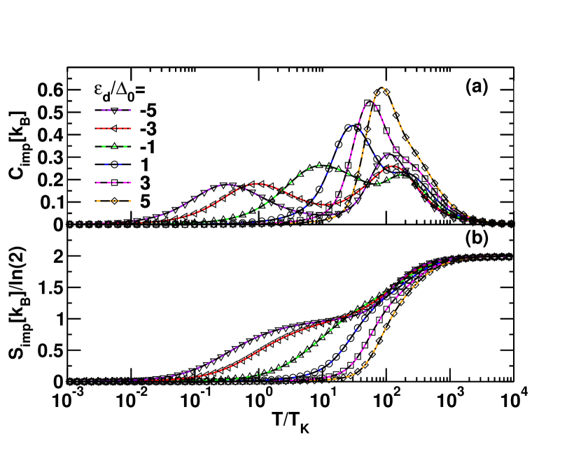
Figure 3: (Color online) (a) Impurity specific heat, $C_{\rm imp}(T)$, and, (b), impurity entropy $S_{\rm imp}(T)$, vs reduced temperature $T/T_{\rm K}$ for the asymmetric Anderson model with $U/\Delta_{0}=12$, $\Delta_{0}=0.001D$ and several values of $\varepsilon_{d}/\Delta_{0}=-5,-3,\dots,+5$. Broken lines: FDM approach. Solid lines: conventional approach. Bethe ansatz results are shown as symbols for $\varepsilon_{d}/\Delta$. For simplicity we used the symmetric $T_{\rm K}$ of Eq. (20) for all $\varepsilon_{d}$ values. NRG and $z$-averaging parameters as in Fig. 1.

Figure 2 shows the impurity specific heat ($C_{\rm imp}$) and impurity entropy ($S_{\rm imp}$) for the symmetric Anderson model versus temperature $T/T_{\rm K}$ for increasing Coulomb interaction $U/\Delta_{0}$. One sees from Fig. 2 that there is excellent agreement between the results obtained within the FDM approach, within the conventional approach and within the exact Bethe ansatz calculations. This agreement is found for both the strongly correlated limit $U/\Delta_{0}\gg 1$ where there are two peaks in the specific heat, a low temperature Kondo induced peak and a high temperature peak due to the resonant level, and for the weakly correlated limit $U/\Delta_{0}\lesssim 1$, where there is only a single resonant level peak in the specific heat. The correct high temperature entropy $\ln 4$ is obtained in all cases.

The temperature dependence of the impurity specific heat and entropy, for the asymmetric Anderson model is shown in Fig. 3 for local level positions ranging from $\varepsilon_{d}/\Delta_{0}=-6$ to $+5$ in units of $\Delta_{0}$. For simplicity we continue to show the results as a function of $T/T_{\rm K}$, with $T_{\rm K}$ the symmetric Kondo scale (20), although, the true Kondo scale will deviate from this for $\varepsilon_{d}>-U/2$. The FDM results agree also here very well with the conventional approach and the Bethe ansatz calculations.

IV.2 Susceptibility and Wilson ratio

Figure 4: (Color online) Impurity susceptibility, $\chi_{\rm imp}(T)$, vs $T/T_{\rm K}$ for the symmetric Anderson model with $U/\Delta_{0}=12,10,8,6,4,2,1,0.01$ and $\Delta_{0}=0.001D$ with $T_{\rm K}$ defined in Eq. (20) for $U/\Delta_{0}\geq 1$ and $T_{K}=\Delta_{0}$ for the $U/\Delta_{0}=0.01$ case. Broken lines: FDM approach. Solid lines: conventional approach. Symbols: Bethe ansatz (for selected values of $U/\Delta_{0}=12,8,6,4,2$). As a guide to the eye, note that $\chi_{\rm imp}$ is increasingly enhanced with increasing $U$. NRG and $z$-averaging parameters as in Fig. 1.

Fig. 4 compares the susceptibilities of the symmetric Anderson model calculated from FDM, conventional and Bethe ansatz approaches for several values of $U/\Delta_{0}$, again indicating good agreement over the whole temperature range between these three approaches.

$U/\Delta_{0}$	$k_{B}T_{K}\chi_{\mathrm{imp}}^{a}/(g\mu_{B})^{2}$		$R^{a}$
	$a=\mathrm{BA}$	$a=\mathrm{NRG}$	$a=\mathrm{BA}$	$a=\mathrm{NRG}$
$12$	$0.250091$	$0.256$	$1.998$	$2.027$
$10$	–	$0.256$	–	$2.024$
$8$	$0.250715$	$0.256$	$1.986$	$2.013$
$6$	–	$0.2574$	–	$1.982$
$4$	$0.259130$	$0.2637$	$1.852$	$1.877$
$2$	–	$0.3085$	–	$1.578$
$1$	–	$0.2214$	–	$1.317$
$0.01$	–	$0.1599$	–	$1.003$

Table 1: Zero temperature susceptibilities $k_{\rm B}T_{K}\chi_{\rm imp}^{a}/(g\mu_{\rm B})^{2}$ and Wilson ratios $R^{a}\equiv\lim_{T\rightarrow 0}4\pi^{2}\chi_{\rm imp}^{a}(T)/3C_{\rm imp}^{a}(T)/T$ for the symmetric Anderson model at several values of $U/\Delta_{0}$ using the Bethe ansatz/NRG FDM approach ($a={\rm BA/NRG}$). Note that $T_{\rm K}$ is defined by Eq. 20 for $U/\Delta_{0}>1$ and is set to $\Delta_{0}$ otherwise.

Table 1 lists the zero temperature impurity susceptibilities ($k_{\rm B}T_{K}\chi_{\rm imp}/(g\mu_{\rm B})^{2}$) and Wilson ratios ($R\equiv\lim_{T\rightarrow 0}4\pi^{2}\chi_{\rm imp}(T)/3C_{\rm imp}(T)/T$), for the symmetric Anderson model as calculated within FDM and for a range of Coulomb interactions from strong $U/\Delta_{0}\gg 1$ to weak ($U/\Delta_{0}\ll 1$). In these two limits, the Wilson ratio for the symmetric Anderson model approaches the well known values of $2$, and $1$, respectively within FDM ($a=NRG$) and Bethe ansatz. Comparison with Bethe ansatz results at selected values of $U/\Delta_{0}$ indicate an error in the susceptibility of around $2\%$ with a similar error in the Wilson ratio.

Figure 5: (Color online) Impurity susceptibility, $\chi_{\rm imp}(T)$, vs $T/T_{\rm K}$ for the asymmetric Anderson model with $U/\Delta_{0}=12$, $\Delta_{0}=0.001D$ and several values of $\varepsilon_{d}/\Delta_{0}$ with $T_{\rm K}$ defined in Eq. (20). Broken lines: FDM approach. Solid lines: conventional approach. Symbols: Bethe ansatz (for selected values of $\varepsilon_{d}/\Delta_{0}=-5,-3,-1,0,+1,+3$). As a guide to the eye, note that the susceptibility curves shift to higher temperatures with increasing $\varepsilon_{d}$. NRG and $z$-averaging parameters as in Fig. 1.

Fig. 5 shows results within FDM and conventional approaches for the asymmetric Anderson model ($\varepsilon_{d}>-U/2$) and for several local level positions ranging from the Kondo ($-\varepsilon_{d}/\Delta_{0}\gg 1$) to the mixed valence $|\varepsilon_{d}/\Delta_{0}|\leq 1$ and empty orbital regimes $\varepsilon_{d}/\Delta_{0}>1$. Bethe ansatz results are also shown for selected local level positions, and we see again very good agreement between all three methods over the whole temperature range. Corresponding zero temperature susceptibilities and Wilson ratios are listed in Table 2. Note that the Wilson ratio approaches the value for a non-interacting system only in the empty orbital limit ($\varepsilon_{d}\gg\Delta_{0}$), being approximately $1.5\pm 0.25$ in the mixed valence regime ($|\varepsilon_{d}/\Delta_{0}|\lesssim 1$). The Wilson ratio from NRG and Bethe ansatz deviate by less than $3\%$ in all regimes.

$\varepsilon_{d}/\Delta_{0}$	$k_{B}T_{K}\chi_{\mathrm{imp}}^{a}/(g\mu_{B})^{2}$		$R^{a}$
	$a=BA$	$a=NRG$	$a=BA$	$a=NRG$
$-5$	$0.219482$	$0.2245$	$1.999$	$2.025$
$-4$	–	$0.1515$	–	$2.023$
$-3$	$0.077356$	$0.0785$	$1.990$	$2.00$
$-2$	–	$0.0315$	–	$1.97$
$-1$	$0.010337$	$0.0103$	$1.795$	$1.78$
$0$	$0.003303$	$0.0033$	$1.512$	$1.50$
$1$	$0.001250$	$0.0013$	$1.315$	$1.32$
$2$	–	$0.00059$	–	$1.18$
$3$	$0.000325$	$0.00033$	$1.086$	$1.12$
$4$	–	$0.00021$	–	$1.09$
$5$	–	$0.00014$	–	$1.06$

Table 2: Zero temperature susceptibilities $k_{\rm B}T\chi_{\rm imp}^{a}/(g\mu_{\rm B})^{2}$ and Wilson ratios $R^{a}\equiv\lim_{T\rightarrow 0}4\pi^{2}\chi_{\rm imp}^{a}(T)/3C_{\rm imp}^{a}(T)/T$ for the asymmetric Anderson model at $U/\Delta_{0}=12$ and several local level positions $\varepsilon_{d}/\Delta_{0}$ using the Bethe ansatz/FDM NRG approach ($a={\rm BA/NRG}$).

IV.3 Local susceptibility

It is also interesting to consider the susceptibility, $\chi_{\rm loc}$, in response to a local magnetic field acting only at the impurity site and to compare this with the susceptibility, $\chi_{\rm imp}$, discussed above, in which the magnetic field acts on both the impurity and conduction electron spins. The former is relevant, for example, in nuclear magnetic resonance and neutron scattering experiments, while the latter can be measured in bulk samples with and without magnetic impurities.

A local magnetic field term, $-g\mu_{\rm B}BS_{\rm z,d}$, in the Anderson model, with $S_{z,d}=(n_{d\uparrow}-n_{d\downarrow})/2$, is not a conserved quantity, i.e $S_{\rm z,d}$ is not conserved , and $\chi_{\rm loc}(T)$ cannot be expressed as a fluctuation as in Eq. (3-4), which would obviate the need to explicitly evaluate a numerical second derivative with respect to $B$ of the thermodynamic potential. Such a derivative, however, poses no actual problem within NRG, so we proceed by explicitly diagonalizing the Anderson model in a local field, using only ${\rm U}(1)$ symmetries for charge and spin (for the symmetric Anderson model in a magnetic field, an ${\rm SU}(2)$ pseudo-spin symmetry may be exploited, by using the mapping of this model in a local magnetic field $B$ onto the ${\rm SU}(2)$ invariant negative-$U$ Anderson model in zero magnetic field at finite level asymmetry $2\varepsilon_{d}+U=B$ Iche and Zawadowski (1972); Hewson et al. (2006)). The evaluation of $\chi_{\rm loc}$ then proceeds via $\chi_{\rm loc}(T,B=0)=-\partial^{2}\Omega_{\rm loc}(T,B)/\partial B^{2}|_{B=0}$ where $\Omega_{\rm loc}(T,B)=\Omega(T,B)-\Omega_{\rm 0}(T)$ and $\Omega(T,B)$ and $\Omega_{\rm 0}(T)$ are the thermodynamic potentials of the total system in a local magnetic field $B$ and the host system, respectively.

Results for $\chi_{\rm loc}$ obtained in this way are shown in Fig. 6 at several values of $U/\Delta_{0}$ as a function of $T/T_{\rm K}$. A comparison of $\chi_{\rm loc}$ to $\chi_{\rm imp}$ obtained from the Bethe ansatz, allows us to conclude that these two susceptibilities are close to identical at all temperatures, i.e. $\chi_{\rm imp}(T)=\chi_{\rm loc}(T)$ and for all interaction strengths $U/\Delta_{\rm 0}$. This is not always the case. A prominent example is the anisotropic Kondo model Vigman and Finkelstein (1978), where $\chi_{\rm imp}=\alpha\chi_{\rm loc}$, with the dissipation strength $0\leq\alpha\leq 1$ being determined by the anisotropy of the exchange interaction Vigman and Finkelstein (1978); Guinea et al. (1985).

Figure 6: (Color online) Comparison of the local, $\chi_{\rm loc}(T)$, and impurity, $\chi_{\rm imp}$, susceptibilities vs $T/T_{\rm K}$ for the symmetric Anderson model with $U/\Delta_{0}=12,8,4,2$ and $\Delta_{0}=0.001D$ with $T_{\rm K}$ defined in Eq. (20). Broken lines: FDM approach. Symbols: Bethe ansatz (for selected values of $U/\Delta_{0}=12,8,4,2$). NRG and $z$-averaging parameters as in Fig. 1.

Figure 7 compares local and impurity susceptibilities for the asymmetric Anderson model in the strong correlation limit ($U/\Delta_{\rm 0}=12$) for several local level positions, ranging from the Kondo ($\varepsilon_{d}/\Delta_{0}=-5,-4,-3,-2$) to the mixed valence ($\varepsilon_{d}/\Delta_{0}=-1,0,+1$) and into the empty orbital regime ($\varepsilon_{d}/\Delta_{0}=+2,\dots,+5$). We see that, as for the symmetric Anderson model, local and impurity susceptibilities are almost identical at all temperatures and for all local level positions, i.e. $\chi_{\rm imp}(T)=\chi_{\rm loc}(T)$ for the parameter values used.

Figure 7: (Color online) Comparison of the local, $\chi_{\rm loc}$, and impurity, $\chi_{\rm imp}(T)$, susceptibilities vs $T/T_{\rm K}$ for the asymmetric Anderson model with $U/\Delta_{0}=12$, $\Delta_{0}=0.001D$ with $T_{\rm K}$ defined in Eq. (20) and for several values of the local level position: $\varepsilon_{d}/\Delta_{\rm 0}=-5,-4,\dots,+5$. Broken lines: $\chi_{\rm loc}$ from the FDM approach. Symbols: $\chi_{\rm imp}$ from Bethe ansatz for selected values of $\varepsilon_{d}$. The NRG calculations are for $\Lambda=4$ with an energy cut-off $e_{c}(\Lambda=4)=40$ with $z$-averaging [$n_{z}=2$ with $z=0$ and $z=0.5$].

The result $\chi_{\rm imp}(T)=\chi_{\rm loc}(T)$, which we verified here, follows from the Clogston-Anderson compensation theoremClogston and Anderson (1961) (see Ref. Hewson, 1997). Consider the impurity contribution to the magnetization $M_{\rm imp}(B)$ in a uniform field. This is given by $M_{\rm imp}/(g\mu_{\rm B})=\langle S_{z,d}+S_{z,c}\rangle-\langle S_{z,c}\rangle_{\rm 0}$ where $S_{z,d},S_{z,c}$ are the impurity and conduction electron $z-$components of spin. Using equations of motion, one easily shows Hewson (1997), that the additional impurity magnetization $\delta M_{\rm imp}/(g\mu_{\rm B})=\langle S_{z,c}\rangle-\langle S_{z,c}\rangle_{\rm 0}$ from the conduction electrons induced by the presence of the impurity is given by

$$\frac{\delta M_{\rm imp}}{(g\mu_{\rm B})}=\frac{1}{2\pi}\sum_{\sigma}\int d\omega f(\omega){\rm Im}\left[\sigma G_{d\sigma}(\omega,B)\frac{\partial\Delta(\omega)}{\partial\omega}\right],$$ (21)

where $f(\omega)$ is the Fermi function, $G_{d\sigma}(\omega,B)$ is the spin $\sigma$ local level Green function of the Anderson model and $\Delta(\omega)=\sum_{k}|V_{k}|^{2}/(\omega-\epsilon_{k}+i\delta)$ is the hybridization function. For a flat band, $\partial\Delta(\omega)/\partial\omega\approx\Delta_{0}/D$ in the wide-band limit. Hence, $\delta M_{\rm imp}/(g\mu_{\rm B})$ is of order $(M_{\rm loc}(B)/g\mu_{\rm B})\Delta_{0}/D$ where $M_{\rm loc}(B)/(g\mu_{\rm B})=\langle n_{d\uparrow}-n_{d\downarrow}\rangle/2=\langle S_{z,d}\rangle$ is the local magnetization, which is linear in $B$ for $B\rightarrow 0$. From this we deduce that $M_{\rm imp}/(g\mu_{\rm B})\approx\langle S_{z,d}\rangle\equiv M_{\rm loc}/(g\mu_{\rm B})$ to within corrections of order $(M_{\rm loc}(B)/g\mu_{\rm B})\Delta_{0}/D$, i.e. $\chi_{\rm imp}(T)=\chi_{\rm loc}(T)$ to within corrections of order $(\chi_{\rm loc}(T)/(g\mu_{\rm B})^{2})\Delta_{0}/D\ll\chi_{\rm loc}(T)$. Away from the wide-band limit, or for strong energy dependence of $\Delta(\omega)$, the above susceptibilities will differ by the correction term given by the field derivative of $\delta M_{\rm imp}$ in Eq. (21).

IV.4 Double occupancy

Figure 8: (Color online) (a) Double occupancy $D_{\rm occ}=\langle n_{d\uparrow}n_{d\downarrow}\rangle$ as a function of temperature $T/T_{\rm K}$ for the symmetric Anderson model and decreasing values of $U/\Delta_{0}=12,10,8,6,4,2,1,0.01$ within FDM (solid lines) and conventional approaches (symbols). (b) Double occupancy $D_{\rm occ}=\langle n_{d\uparrow}n_{d\downarrow}\rangle$ as a function of temperature $T/T_{\rm K}$ for the asymmetric Anderson model and increasing values of $\varepsilon_{d}/\Delta_{0}=-5,-3,-1,0,+1,+3,+5$ for $U/\Delta_{0}=12$ within FDM (solid lines) and conventional approaches (symbols). $T_{\rm K}$ is defined in Eq. (20) for $U/\Delta_{0}\geq 1$ and is set to $\Delta_{0}$ for the case $U/\Delta_{0}=0.01$. NRG and $z$-averaging parameters as in Fig. 1.

Our conclusions concerning the accuracy of specific heat and the susceptibility calculations within the FDM approach, hold also for other thermodynamic properties, e.g. for the occupation number or the double occupancy. Fig. 8(a) shows a comparison between the FDM and conventional approaches for the temperature dependence of the double occupancy $D_{\rm occ}=\langle n_{d\uparrow}n_{d\downarrow}\rangle$ of the symmetric model for different strengths of correlation $U/\Delta_{0}$, and Fig. 8(b) shows the same for the asymmetric Anderson model for $U/\Delta_{0}=12$ and for several local level positions. The results of the two approaches agree at all temperatures, local level positions and Coulomb interactions. Notice that $D$ acquires its mean-field value of $1/4$ for the symmetric model in the limit $U/\Delta_{0}\rightarrow 0$ and is strongly suppressed with increasing Coulomb interaction away from this limit [see Fig. 8(a)]. Similarly for the asymmetric model, increasing $\varepsilon_{d}/\Delta_{0}$ away from the correlated Kondo regime decreases the double occupancy significantly [see Fig. 8(b)].

V Summary

In this paper we focused on the calculation of the impurity specific heat and the impurity susceptibility of the Anderson model within the FDM approach Weichselbaum and von Delft (2007), finding that this method gives reliable results for these quantities, as shown by a comparison to both exact Bethe ansatz calculations Kawakami and Okiji (1981, 1982); Okiji and Kawakami (1983); Wiegmann and Tsvelick (1983); Tsvelick and Wiegmann (1983); Filyov et al. (1982); Tsvelick and Wiegmann (1982) and to NRG calculations within the conventional approach Campo and Oliveira (2005). Some care is needed in implementing the FDM approach for the susceptibility $\chi_{\rm imp}$ in a uniform field, i.e. when the applied magnetic field acts on both the impurity and conduction electron spins. In this case, an additional contribution from the environment degrees of freedom needs to be included. We also showed that the susceptibility in response to a local magnetic field on the impurity, $\chi_{\rm loc}$, could also be obtained within FDM and a comparison of this susceptibility with $\chi_{\rm imp}$ (from Bethe ansatz), showed that they are close to identical at all temperatures, and in all parameter regimes for $\Delta_{0}\ll D$, thereby verifying the Clogston-Anderson compensation theorem. An arbitrary temperature grid can be used for thermodynamics in both the conventional and the FDM approaches, however, the former requires a specific best shell to be selected depending on $T$ and $z$, whereas the FDM approach avoids this step by incorporating all excitations from all shells in a single density matrix.

We also showed, that quantities such as the double occupancy can also be accurately calculated within the FDM approach. The double occupancy can be probed in experiments on cold atom realizations of Hubbard models in optical lattices. Jördens et al. (2008); Schneider et al. (2008) Flexible techniques, such as the FDM approach, for calculating them within a dynamical mean field theory Kotliar and Vollhardt (2004); Georges et al. (1996); Vollhardt (2012) treatment of the underlying effective quantum impurity models could be useful in future investigations of such systems Tang et al. (2012).