Intriguing solutions of the Bethe-Salpeter equation for radially excited pseudoscalar charmonia

Abstract

The purpose of this paper is twofold. The first purpose is to find a fully Poincare invariant solution of the Bethe-Salpeter equation for excited quarkonia, however, the second, in fact, major focus is on the relevance of the space-time metric choice and its imapact on the correct description of the ground and all excited states. For the first time, we compare BSE solutions defined independently with Euclidean and Minkowski metric. For this purpose, the BSE is conventionally defined and solved in Euclidean space with two versions of the propagator : the bare propagator and the confined form of the quark propagator with complex conjugated poles. In both considered cases, there is unexpected doubling of the spectrum, when comparing to the experiments as well as to the solutions of the Schrodinger equation. The quark propagator with complex conjugated singularities allows us to find the BSE solution directly in Minkowski momentum space as well. We find the Minkowski space solution for confining theories is not only numerically accessible, but provides a reliable, albeit not yet completely satisfactory, description of the ground and excited meson states.

I Introduction

Excited meson spectroscopy is a keystone experimental output, which is essential for understanding quark-antiquark interaction. The dynamics of hadrons is dominantly driven by the solely known strongly interacting quantum field theory- quantum chromodynamics. The confining forces are responsible for the absence of colored hadron constituents and simultaneously they lead to the spectra of ground state mesons and excited resonances. Because of the strong interaction at large distances $r\simeq 1/{\Lambda_{QCD}}$, the use of Schrodinger equation becomes meaningless for light hadrons. Unlike to the potential quantum-mechanical description, the excited states are not described by an orthogonal wave function in quantum field theory.

More precisely, within the model of logarithmic confinement QUIROS1979 ; EIMARO2007 , one has $<v^{2}>=0.24$ for quark of mass $m_{c}=1.5$GeV bounded inside of $1S$ charmonia. Thus, charmonia lie on the borderline of a nonrelativistic description applicability (while this is less urgent for bottomonia, where one has $<v^{2}>=0.08$ for the ground state). In fact, one requires the use of quantum field description in order to maintain Lorentz invariance, however most of the results (e.g. spectroscopy) still should be consistent with usual quantum-mechanical machinery. In this respect, the physics of charmonia represent exciting theoretical laboratory where various methods can coexist.

Recently in the CLEO CLEO and Belle experiments progress in the experimental determination of electromagnetic transitions has provided new data, which should be confronted with fully Poincare invariant description. Recall that in naive quantum mechanical quarkonium picture $\psi(nS)\rightarrow\eta(n^{{}^{\prime}}S)\gamma$ transitions should vanishes in zero recoil $\gamma$ for different $n,n^{{}^{\prime}}$ due to the orthogonality of radial wave functions (see for instance Eichten1975 ; Eichten1980 ). This is not the case of relativistic treatment in Bethe-Salpeter equation (BSE) framework, where this so called ”hindered” transitions are not expected to be vanishing even for small photon energy. Also, a lot is known from heavy quarkonia production in $e^{+}e^{-}$ anihilations, where vector quarkonia are straightforwardly produced. The BABAR BABAR , Belle and BESS experiments continue collection of various meson experimental data.

In quantum field theory the two body bound state is described by the Bethe-Salpeter (BS) vertex function or, equivalently, by the BS amplitudes. Both of them are solutions of the corresponding covariant four-dimensional BSE, which has definite structure dictated by the total spin of the meson. When generalizing recent various quantum-mechanical models to quantum field theoretical approach, one is faced with the solutions that do not exist in the nonrelativistic limit. Some of these states, the so called ghosts, are believed to be an artefact of inconsistent approximations or even illness of the theory at all ALKOFER and we will not discuss these states in this paper. However some of these additional states can not be apriory excluded as they have the same symmetry as expected -physical- ones. For partial simplicity of related BSE structure we have started with pseudoscalar charmonia in this paper, recalling that the heaviest candidate for excited pseudoscalar $\eta_{c}$ meson was $X(3940)$ observed by Belle Belle in double charmonium production is very likely $\eta(3S)$ state.

The experimental data accompanied by quantum mechanical hints of nonrelativistic QCD limit can guide the systematics of hadronic excited states obtained in various different frameworks. Actually we suppose that the charmonium is ideal system, which can be used when concerning and discriminating the properties of strong coupling models defined in different metrics. While it is commonly assumed that QCD formulated within the Minkowski metric and in Euclidean space are equivalent, we will regard Euclidean QCD and Minkowski QCD as independent theories. Let us stress, that having no comparisons in the literature, the equivalence of the Minkowski and Euclidean formulation is very formal. It is believed or assumed that the solution in the timelike Minkowski space can be uniquely obtained from the Euclidean by analytical continuation. While this procedure is well defined in perturbation theory calculus, it is not straightforward in confining theory like QCD. Actually, it has been known for almost a quarter century, that the (light) quark propagator exhibits complex conjugated branch points STACAH1990 and, very similarly, it is assumed for gluons as well STINGL1 ; STINGL2 . Such presence of complex conjugated singularities implies inequivalence of the original Minkowski theory and the theory defined in the Euclidean space. Recall that the usual Wick rotation does not provide correct Euclidean-Minkowski continuation in this case. In order to provide first insights, we start with the historically more usual Euclidean formulation of BSE for charmonia,and we perform a realistic non-perturbative calculation using the Minkowski metric as the defining one. Assuming the Euclidean theory offers good approximation, we use the quark propagator with complex conjugated singularities for the Minkowski space calculation as well. As we will see, contrary to popular belief, the obtained numerical spectrum prefers the Minkowski metric.

In the recent paper JA , vector charmonia have been considered in the approximation with one dominant component. In the present paper, we continue to study for pseudoscalar $c\bar{c}$ mesons by using the BSE model. In the sections II and III, the Euclidean BSE for all components completely included is discussed and the results are presented for an arbitrary excited state for the first time. The states with masses above $3.9$GeV are predictions of our presented BSE model. Section IV is devoted to the novel Minkowski space-time treatment of the BSE for mesons.

II BSE for Pseudoscalar Charmonium in Euclidean space

The BSE for the pseudoscalar meson in Minkowski space reads

$$\Gamma(q,P)=-i\int\frac{d^{4}k}{(2\pi)^{4}}\left[S(q-P/2)\Gamma(p,q)S(q+P/2)\right]^{i,j}V(k,q,P)_{i,k,l,j}\,\,,$$ (1)

where latin letters $i,j...$ represent Dirac indices. Explicitly for the pseudoscalar, we have

$$\Gamma_{P}(q,P)=\gamma_{5}\left(A(q,P)+\not PC(q,P)+\not qB(q,P)+[\not q,\not P]D(q,P)\right)\,\,,$$ (2)

Alternatively, the BSE vertex function can be replaced by a (more singular) BS wave function $\chi$ through its definition

$$\Gamma(q,P)=S^{-1}(q-P/2)\chi(q,P)S^{-1}(q+P/2)\,\,,$$ (3)

which is usually considered when performing the nonrelativistic limit. The interaction kernel is given by the infinite sum of the two-particle irreducible quark-antiquark scattering graphs in a color-anticolor channel.

According to the original idea of Ref. Wilson:1974 , confinement in the heavy flavor hadron sector is typically associated with a linearly rising potential between constituents QUIROS1979 ; Eichten1978 . The spin degeneracy observed in meson spectrum tells us that the confining part of the interaction should be largely spin independent- it should be a Lorentz scalar. Euclidean approximation ofthe lattice calculations leads to various predictions for the potential between heavy quark-antiquark states. For instance, Coulomb gauge potential rises linearly with the slope larger than required by an approximate Regge trajectory of light mesons, while all interpolating gauges between Landau and Coulomb gauge produce potential which is bounded from above SUGANUMA . Also in Refs. DICHAQI ; Licha2009 ; Zhang ; Chao1 ; Chao2 ; Vento2011 , it has been found that the meson spectroscopy is better described by a ”confining” potential which is bounded from above. Irrespective of the gauge, the flatness of linearly rising potential arises from the string breaking scenario: including light quarks into the game then the creation of the quark-antiquark pairs, i.e. pions and other light mesons are energetically favorable. Such screening is in agreement with observed high radially excited heavy mesons- without any doubt, the spectrum deviates from the linear Regge trajectory. According to nonrelativistic quantum mechanic predictions, the relatively small hyperfine and fine-structure splitting in quarkonium levels is due to the Lorentz vector part of the interquark interaction Appelquist1978 ; Novikov1978 ; Kwong1987 ; Brambilla2004 , which should be added for a more accurate description. Following the arguments stated here the dominant part of $V$ should be a Lorentz scalar, and further vectorial interaction is naturally assumed in QCD (for a quarkonia mainstream, see Ref. QUARKONIA ). The interaction phenomenologically chosen here, thus, reads

$$V(k,q,P)_{iklj} = 1_{ik}1_{lj}V_{s}+\gamma_{\mu,ik}\gamma^{\mu}_{lj}V_{v}\,\,,$$

$$V_{s} = \frac{\kappa_{s}}{(q^{2}-\mu_{s}^{2})^{2}}\,\,$$

$$V_{v} = \frac{g^{2}}{q^{2}-\mu_{v}^{2}}\,\,.$$ (4)

Note the scalar part corresponds with the negative exponential potential in the nonrelativistic limit, $V_{s}({\bf r})\simeq-e^{-r\mu_{s}}$.

The color Coulomb potential is usually taken due to the exchange of the gluon. It should reflect the freezing of the effective coupling in the infrared related with the gluon propagator suppression due to the soft gluon mass generation Mendes ; PBC1 ; PBC2 through the Yang-Mills Schwinger mechanism. Here, we simplify and approximate $V_{v}$ by a constant coupling and constant gluon mass of expected size $\mu_{v}\simeq\Lambda_{{\mbox{Q}CD}}$. Further, from the string models, it is well known that the string tension changes with the scale as well. At least, it is considerably larger for the charmonium than for the bottomonium. Here we found advantageous to consider such running already for different charmonia, and we simply separate the $1S$ state from the others in the following way:

$$\kappa_{s}=\kappa\left[\theta(P^{2}-M^{2}(1s))+\delta\theta(-P^{2}+M^{2}(1s))\right]\,$$ (5)

where numerically, $\delta=0.9$.

We formally start at Minkowski space and transform 16 component of BSE into the coupled set of four integral equations for four components $A,B,C,D$. The Wick rotation and further details are discussed in the appendices.

heeeeeeeeeerrrrrrrrrrrrrre is the end

III Numerical method and results

Independent of the details of the model, when solving BSEs in the Euclidean space, we face a rather intriguing problem, which we call the doubling of excited states. With the exception of the ground state (and possibly, the 2s state) there are 2 times more excitations than in the nonrelativistic limit (for the nonrelativistic limit, see, for instance Licha2009 ; Chao1 ; Chao2 ; Vento2011 ). We have found that the doubling is numerically stable, and we argue that this is a rigid property of the BSE numerical solution for heavy quarkonia in the Euclidean space.

Let us discuss the doubling phenomena in more detail. It is a matter of the fact that instead of one excited state, we observe an emergence of two with very similar BSE wave functions. The appropriate numerical procedure is described in Appendix B with a typical result shown in Figs. 6 and 7. As it is explained in the Appendix B, we introduce the auxiliary eigenvalue function $\lambda$ in a way that whenever $\lambda$ crosses the unit, we get a bound state. As mentioned, the doublets are characterized by an almost identical vertex function, hence, they are physically distinguishable only by a slightly different $M$ . Numerically, they have been found as a neighborhood energy levels with the opposite derivative $d\lambda/dM$. As we will discuss below, the appearance of doubling does not depend on whether the free quark propagators approximation or some confined form for the quark propagator is used. Actually, for a reasonable large value of the imaginary part of the complex conjugated mass term, the spectrum of the model with confine quarks is quite similar in both Euclidean models under consideration. Varying the imaginary part of the pole position can shrink the energy gap between the doublet pair; however, it leads to an unacceptable changes of the charmonium spectrum before the doubling is eliminated. We infer that the phenomena of energy doubling is not related solely with analytical properties of quark propagators, but it is a consequence of the use of Euclidean metric as a definite one.

To get rid of this problem we solve the BSE with two approximations of the quark propagator. The free quark propagator in the first:

$$S(k)=\frac{\not k+m_{c}}{k^{2}-m_{c}^{2}+i\epsilon}\,,$$ (6)

where $m_{c}\simeq 1.5$GeV is the real ”constituent” charm quark mass.

A confined type of quark propagator was used in the second approximation of the BSE in the Euclidean space. The charmonium quark propagator has been approximated by the following formula

$$S(k)=\left[\not k+m\right]\frac{k^{2}-m_{c}^{2}}{(k^{2}-m_{c}^{2})^{2}+\delta^{4}}\,,$$ (7)

which is written in Minkowski space and where $m_{c},\delta$ are real parameters. Such form of the propagator is in accordance with confinement maris1995 ; STINGL1 ; STINGL2 ; DUDAL1 ; DUDAL2 ; lat1 ; lat2 ; CLOROB2013 , and for a quark with momentum ${\bf k}\simeq\delta$, the parameter $\delta$ can be interpreted as minimal wavelength SHROCK . It does not have a real pole corresponding to the free particle solution, but, instead, there are complex conjugated singularities, as wassuggested almost 25 years ago in STACAH1990 .

The change of the free quark propagator into the form (7) is equivalent to replace the double Euclidean propagator $G_{2}$ in (VI) in a way such that $G_{2}\rightarrow G_{new}$, where

$$G_{new}=\frac{I_{free}}{I_{free}^{2}+\delta^{8}+\delta^{4}\left[(k^{2}_{E}-\frac{P^{2}}{4}+m_{c}^{2})^{2}-k_{4}^{2}P^{2}+\lambda_{inf}\right]}\,$$ (8)

and where $I_{free}$ corresponds with the inverse of the original $G_{2}$, i.e.,

$$I_{free}=(k^{2}_{E}-\frac{P^{2}}{4}+m_{c}^{2})^{2}+k_{4}^{2}P^{2}\,\,.$$ (9)

Nowadays, up to the first two, the excited pseudoscalars have not been accessible in the experiments. We remind here, that the highest mass candidate suggested is $\eta(3s)$ observed in the Belle experiment in 2007 and hopefully will be confirmed in the future experiments in the recently built FAIR facilities. It is well known that the masses of $0^{-+}$ excited states should be approximately degenerated with $S-states$ vectors charmonia. The five or six s-wave dominated $\psi$ charmonium vectors are recently known with masses spread in the energy range $3-4.5(5)$GeV RUPP . No doubling is observed there and thus we do not expect doubling in the other channels as well. Remind here, the BSE vertex function depends on two variables :$P.q$ and $q^{2}$. Alternatively and conventionally, vertex function can be visualize as a two dimensional manifold above $q_{4}$ and ${\bf q}$ plane. The BSE solution with free quark propagators for $\eta(1S)$ is shown at Fig. 1 for a fixed $p_{4}=0.25$ GeV. The doublets have been actually searched by by comparison of the vertex functions. Examples of a few neighbor excitations are shown in Figs. 2-4. The order of the energy levels are used to label the solutions (from low to high), and the letter represents the components of the BSE vertex function [according to Eq. (2].

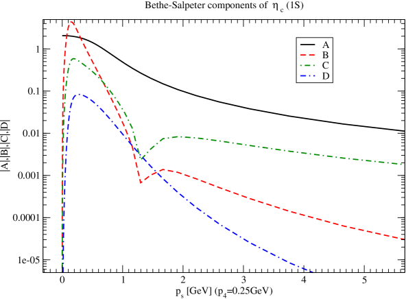
Figure 1: Absolute value of the $A,\beta,C,D$ components of $\eta(1s)$ state. Note the large value of the function $\beta$.

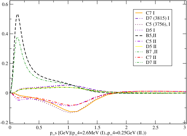
Figure 2: Dependence of components $B,C,D$ on ${\bf k}$ of two excited states shown for two slices with given $k_{4}=2.6MeV$ (I) and $k_{4}=0.25GeV$ (II).

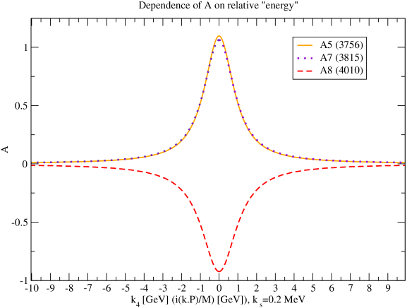
Figure 3: Dependence of dominant component $A$ of three neighbor excited states shown for fixed threemomentum ${\bf{k}}=0.2MeV$. Vertex functions become wider for higher mass of $\eta_{c}$ meson. Quarks ”are more off-shell” in higher excited mesons for the model with a free propagators.

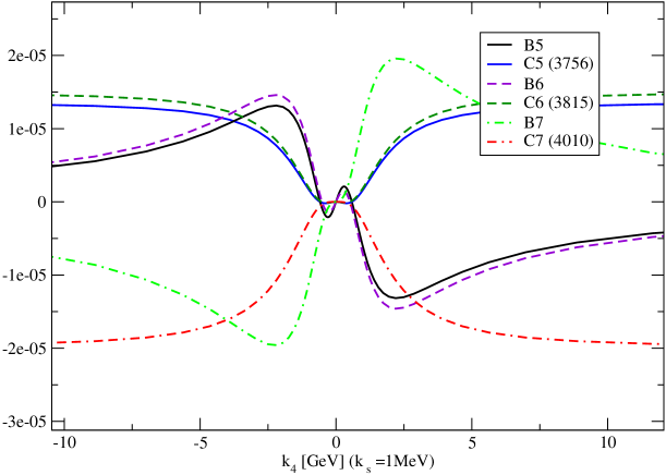
Figure 4: Dependence of B and C components of three excited states shown for fixed threemomentum ${\bf{k}}=0.2$MeV . Levels labeled by B(C)5 (fifth energy excited state) and B(C)6 (sixth excited state) belong to the neighboorhoodhred levels, they have approximately identical vertex functions. They have same nodes (odd function B has three nodes, while C functions have two nodes and zero minimum at beginning, next two higher levels have only one zero, and only the seventh is shown for better visuality).

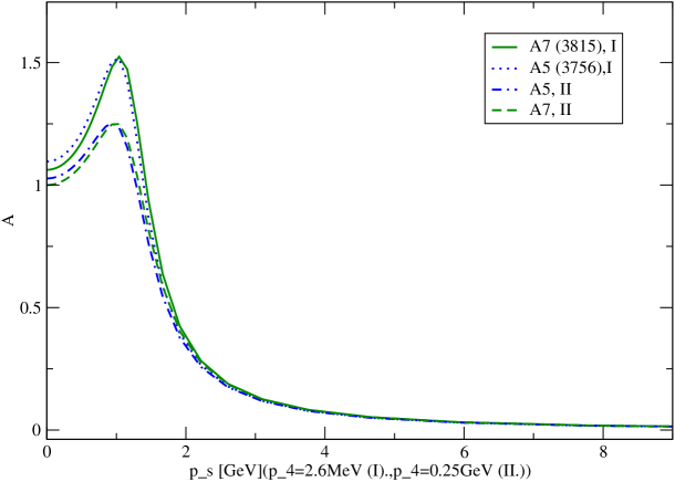
Figure 5: Dependence of dominant component $A$ of two excited states shown for two fixed values $k_{4}=2.6$MeV and $k_{4}=0.25$ GeV. The function $A$ has no nodes for Euclidean relative momentum $k$.

For a rough estimate of the spectra in the case of BSE with free propagators, we adjusted charm quark pole mass to be $m_{c}=1.5$ GeV and we were searching for the charmonium spectra for different parameters $\kappa(P),\mu$. The strength of the effective vectorial interaction $\alpha_{s}=g^{2}/(4\pi)$ has been adjusted in order to adjust the intercept to the experimentally known value $\eta(2s)-\eta_{c}(1s)=660$GeV. According to the nonrelativistic calculations we were varying the parameters $\kappa$ between $2-4GeV^{2}$ and $\mu=0.1-0.5$GeV. At the end the the numerical data have been rescaled in order to get correct value of the ground state exactly. The resulting search is presented in the Table 1. , where the all pairs belonging to the single nonrelativistic counterpartner are matched. In the case of free quark propagator approximation all states are realized above naive quark threshold.

$m_{c}=1500$	$m_{c}=1442$	$<>$	Exp.
3100	2980	2980	2980 (1s)
3785	3638	3638	3638 (2s)
3940	3787
3990	3835	3811	3940* (3s)
4160	4000
4235	4071	4036	- (4s)
4430	4259
4535	4360	4310	-(5s)
4790	4373
4925	4734	4554	-(6s)
5270	5066
5435	5224	5145	-(7s)

Table 1: Conventional BSE solutions for $\eta_{c}(nS)$ for the model with the free quark propagator. We use conventional quantum mechanical assignment $nS$ in order to label states that we expect in nonrelativistic or ”instantaneous” approximations. The first column represent actual numerical solution in units where $m_{c}=1.5GeV,\kappa=2.849GeV^{2}$, in the second column the experimental value of $\eta(1S)$ has been used to scale other levels. The doubling appears for the states $n>2$, and the energy doublets are identified by comparison of vertex functions (e.g. by number of nodes in $B,C,D$ functions). After rescaling we produce experimentally known $\eta(2S)$. For other states -to make levels meaningfully comparable with quantum mechanical labeling- the masses of energy levels are averaged for given energy doublets. $\alpha_{s}=0.07407$ . *Belle observed X(3940) in $e^{+}e^{-}\rightarrow J/\psi+X$, for the interpretation see EIMARO2007 .

For the purpose of numerical study of BSE with confinement incorporated through Eq. (7), we have used the same parameters as in the case for BSE with free propagators, e.g. the real part of the complex poles is $m_{c}=1.5$GeV. The parameter $\delta$ characterizes the splitting of complex conjugated poles and we present the results for two values $\delta=0.6$GeV and $\delta=1.0V$GeV graphically in Fig. 6. The situation for highly excited states is quite similar to the case with unconfined quarks. However, there are new states arising where just only one -$\eta(2)$- should exists, to be more precise there are two new (4 because of doubling) states for $\delta=0.6Gev$ and three (six) additional states for $\delta=1GeV$. While the gaps between the partners of energy doublet slightly and tentatively shrink, the appearance of new states makes any value of $\delta$ inappropriate for a realistic Euclidean model.

Another numerical observation is that the vectorial interaction must be largely suppressed in our model, which gives typical value estimate $\alpha_{s}\simeq 0.07-0.1$. This is several times smaller then the expected value of the strong coupling in nonrelativistic models, where, typically, one gets $\alpha_{s}(m_{c})=0.5$. It is difficult to trace the source of such large suppression. We have explicitly checked that the introduction of the running strong coupling does not explain its suppression in presented model. A more complete understanding of this problem remains for a future study. For a ground state mesons, it is well known that the function $A$ largely dominates. We have found that this is the case for excited mesons as well. This is apparent from the Fig. 7 , where the numerical results are graphically compared for BSE with free propagator.

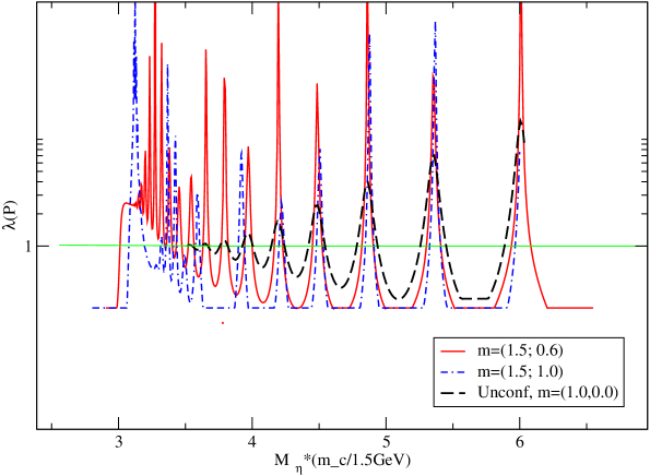
Figure 6: Comparison of BSE solution within various approximation, the solid line represents free quark propagator approximation with $m_{c}=1.5GeV$, the dashed line and dot-dashed line correspond with confined quark propagator characterized by two complex conjugated poles with located at $m_{c}=1.5GeV\pm i0.6GeV$ and $m_{c}=1.5GeV\pm i1.0GeV$ respectively. The BSE has solution whenever a curve crosses the horizontal solid line. Energy doublets corresponds with crosses, which cuts the upper parts of each curve separately.

IV BSE Minkowski space solution with confining propagators

It is obvious that the propagator (7) is a regular function for a real Minkowski variable $k^{2}$. It allows us to consider and explicitly numerically solve the analogue problem in the Minkowski space directly. We completely avoid the use of Euclidean metric by using the confined form of the propagator as in the previous case, however, for now, we stay in the Minkowski space-time. We will use the following convention $k^{2}=k_{\mu}k_{\nu}g^{\mu\nu}=k_{0}^{2}-k_{1}^{2}-k_{2}^{2}-k_{3}^{2}$, and we take for the quark propagator,

$$S(k)=f\left[\not k+m\right]\frac{k^{2}-m_{c}^{2}}{(k^{2}-m_{c}^{2})^{2}+\delta^{4}}\,,$$ (10)

where, in general, $f$ is complex function of the momenta, which, in accordance with the perturbation theory, must become a real valued function for a large spacelike $k$ (recall here that the Dyson-Schwinger equations for propagators are not directly numerically soluble in momentum Minkowski space SAULISDE ). Here, in order to approximate its infrared behavior only, we simplify and take the following constant phase approximation:

$$f={\mbox{e}xp}^{i\frac{\pi}{2}}\,.$$ (11)

To make a comparison meaningful we keep the Lorentz structure of the kernel as in the previous Euclidean study, however in order to make the model tractable, we change the double pole of the scalar kernel to the double pair of complex conjugated poles while leaving the vectorial interaction in its original form (without a Feynman epsilon), explicitly written as

$$V_{s} = \frac{\kappa}{(q^{2}-\mu_{s}^{2})^{2}+\lambda_{s}^{4}}\,\,,$$

$$V_{v} = \frac{g^{2}}{q^{2}-\mu_{v}^{2}}\,\,.$$ (12)

It is worth mentioning that the Minkowski space-time BSE represents well-defined numerical problem, and the convergence is further enforced due to the asymptotic of the vertex function $\Gamma\simeq 1/q^{2}$ at large $q^{2}$ . In this way, the BSE turns out to be two-dimensional integral equation for two real variables: two scalars $k^{2},k.P$ for given discrete $P^{2}=M^{2}$, or alternatively, for the off-shell relative energy $k_{0}$ and spacelike relative momentum ${\bf k}$. According to our Euclidean space founding we keep only the component $A$ as a reasonable approximation of the full BSE amplitude. The BSE in Minkowski space has been solved numerically in a very similar fashion as in the previous Euclidean case. Note also, that due to our simplifications, the Minkowski vertex function remains real valued in the entire Minkowski space.

To specify the rest, we put $\mu_{s}=\mu_{v}=\mu=0.25$GeV and take $\lambda_{s}=2\mu$ for the purpose of our numerical search. Having the double pole of $V_{s}$ changed to the complex conjugated poles, the interaction strength is effectively suppressed. Within a given value of $\lambda_{s}$, one needs to increase the scalar coupling strength. Numerically, now we take $\kappa=5GeV^{2}$ and for the vector, we take $g^{2}=1.8849$. Within $m_{c}=1.5GeV$ the spectrum we have found reads (without any further tuning): $M(1s)=1.97GeV;M(2s)=3.563GeV;M(3s)=4.163GeV;M(4s)=5.9GeV;M(5s)=6.68GeV$. The doubling of energy levels in the numerical solution of the BSE has disappeared. The intercept is presented, although it is overestimated. We believe that quantitative disagreement with the experiment will be further minimized after a further refinement of the parameters used in the presented model and/or after a further improvement of the approximation made.

V Conclusion

The homogeneous BSE for excited states of pseudoscalar charmonia have been solved in the framework of BSE defined in Euclidean and Minkowski space-time independently. A high number of excited states has been found by the numerical solution of the BSE in both spaces, and the numerics has been described in detail here. For those who are interested, the codes are available by an email request. We have found that the excited states are overpopulated when calculated in the Euclidean space. The excited states come in pairs with close masses and almost identical wave functions. This doubling phenomena is very likely an artifact of the Euclidean space approximation. In the Minkowski space-time model with confining-type of the quark propagators, the doubling phenomena of the energy levels disappears. At the recent stage the Minkowski BSE model suffers by the simplifications and approximations made, and it does not reproduce the experimental data precisely. Nevertheless, it is reliable enough to exhibit the Minkowski space metric can be used as a definite metric for nonperturbative QCD calculations as a phenomenological, if not a preferable then certainly an acceptable, choice.

VI Appendix A: Projecting Euclidean BSE with the free fermion propagator

After the projection by $\frac{1}{4}{\mbox{T}r}\gamma_{5}$ we get in Minkowski space :

$$A(q,P) = i\int\frac{d^{4}k}{(2\pi)^{4}}K_{A}(V_{S}-4V_{V})$$

$$K_{A} = S_{V}(-)S_{V}(+)\left[-A(k,P)\left(k^{2}-\frac{P^{2}}{4}\right)+2D(k,P)\left(k^{2}P^{2}+(k.P)^{2}\right)\right]$$ (13)

$$+ S_{S}(-)S_{S}(+)A(k,P)+S_{V}(-)S_{S}(+)\left(k.PB(k,P)-\frac{P^{2}}{2}C(k,P)\right)\,\,,$$

where we have introduced the shorthand notation $S(\pm)=S(k\pm P/2)$. Projecting the BSE by ${\mbox{T}r}\frac{\not q\gamma_{5}}{4}$ one gets

$$q^{2}B(q,P)+q.PC(q,P)=i\int\frac{d^{4}k}{(2\pi)^{4}}\left(q.PK_{B1}+q.kK_{B2}\right)(V_{S}+2V_{V})$$

$$K_{B1} = S_{v}(-)S_{v}(+)\left[\frac{k.P}{2}B(k,P)+\left(k^{2}+\frac{P^{2}}{4}\right)C(k,P)\right]+S_{s}(-)S_{s}(+)C(k,P)-4k^{2}S_{v}(-)S_{s}(+)D(k,P)$$

$$K_{B2} = -S_{v}(-)S_{v}(+)\left[2k.PC(k,P)+\left(k^{2}+\frac{P^{2}}{4}\right)B(k,P)\right]+S_{s}(-)S_{s}(+)B(k,P)+4k.PS_{v}(-)S_{s}(+)D(k,P)\,\,.$$ (14)

Projecting BSE by $Tr\frac{\not P\gamma_{5}}{4}$ one gets in Minkowski space,

$$q.PB(q,P)+C(q,P)P^{2}=i\int\frac{d^{4}k}{(2\pi)^{4}}K_{C}(V_{S}+2V_{V})$$

$$K_{C} = -S_{v}(-)S_{v}(+)B(k,P)k.P(k^{2}-P^{2}/4)+S_{s}(-)S_{s}(+)B(k,P)k.P$$ (15)

$$- S_{v}(-)S_{v}(+)C(k,P)\left[2(k.P)^{2}-k^{2}P^{2}-\frac{P^{2}}{4}\right]+S_{s}(-)S_{s}(+)C(k,P)P^{2}-S_{v}(-)S_{s}(+)A(k,P)P^{2}\,\,,$$

where we have dropped out the trivial term proportional to $D$ due to the identity $S_{V}(-)S_{V}(+)-S_{V}(+)S_{V}(-)=0$. Finally the ”equation for $D$” reads

$$4\left[(q.P)^{2}-q^{2}P^{2}\right]D(q,P)=i4\int\frac{d^{4}k}{(2\pi)^{4}}K_{D}(P.qP.kV_{S}-P^{2}(k.q)V_{S})$$

$$K_{D} = S_{V}(-)S_{V}(+)\left[\frac{A(k,P)}{2}+(k^{2}-P^{2}/4)D(k,P)\right]-S_{V}(-)S_{S}(+)C(k,P)+S_{S}(-)S_{S}(+)D(k,P)\,\,.$$ (16)

To find the solution numerically, it is convenient to perform Wick rotation in the relative momenta, while keeping $P^{2}$ real and positive. In the rest frame of quarkonium $P=(M,0,0,0)$ and after the continuation $q_{o}\rightarrow iq_{4}$ we get for the ”Euclidean” Eq. (VI):

$$A(q,P) = \int\frac{d^{4}k_{E}}{(2\pi)^{4}}U_{A}G_{2}(V_{S}-4V_{V})$$

$$U_{A} = A(k,P)\left(k^{2}_{E}+\frac{P^{2}}{4}+m_{c}^{2}\right)+2D(k,P)\left(-k^{2}_{E}P^{2}+{(k_{4}M)}^{2}\right)+m_{c}k_{4}M\beta(k,P)-m_{c}\frac{P^{2}}{2}C(k,P)\,,$$ (17)

where $A(q,P),U_{A},...$ are the functions of Euclidean momentum $q_{E}=(iq_{0},{\bf q})=(q_{4},{\bf q})$ and Minkowski momentum $P$. From now on we restrict to the use of the free quark propagator

$$S^{-1}(l)=\not l-m_{c}\,,$$ (18)

and introduce shorthand notation for the product of the propagators

$$G_{2}=S_{v}(-)S_{v}(+)\,.$$ (19)

Thus, we can simply write

$$S_{s}(-)S_{s}(+)=m_{c}^{2}G_{2}\ \ \,\ \ S_{v}(-)S_{s}(+)=m_{c}G_{2}\,,$$ (20)

whose identities we will use from the next.

It is easy to find that $G_{2}$ is the product of two complex scalar propagators , which for equal mass case, becomes purely real,

$$G_{2}=\left[(k^{2}_{E}-\frac{P^{2}}{4}+m_{c}^{2})^{2}+k_{4}^{2}P^{2}+\lambda_{inf}\right]^{-1}\,\,,$$ (21)

where we have introduced infrared regulator $\lambda_{inf}<<m_{c},M$ for a later numerical purpose. Furthermore, we have introduced new real function $\beta$ as

$$\beta=iB\,,$$ (22)

which reflects the fact that the function $B$ is odd in the variable $k.P=ik_{4}P$ (valid for a positive $C$ parity eigenstate).The functions $A,\beta,C$ and $D$ are then manifestly real. For the purpose of completeness, we write the Euclidean Eqs. (VI,VI,VI,VI) here

$$q^{2}_{E}\beta(q,P)+q_{4}MC(q,P) = \int\frac{d^{4}k_{E}}{(2\pi)^{4}}\left(q_{4}MU_{B1}+q_{E}.k_{E}U_{B2}\right)(V_{S}+2V_{V})G_{2}$$

$$U_{B1} = \frac{k_{4}M}{2}\beta(k,P)+\left(-k_{E}^{2}+\frac{M^{2}}{4}+m_{c}^{2}\right)C(k,P)+4m_{c}k^{2}_{E}D(k,P)$$

$$U_{B2} = \left(k_{E}^{2}-P^{2}/4+m_{c}^{2}\right)\beta(k,P)+2k_{4}MC(k,P)-4k_{4}Mm_{c}D(k,P)$$ (23)

$$\left[q_{4}\beta(q,P)+C(q,P)M\right] = \int\frac{d^{4}k_{E}}{(2\pi)^{4}}U_{C}(V_{S}+2V_{V})G_{2}$$

$$U_{C} = k_{4}(k_{E}^{2}+\frac{P^{2}}{4}+m_{c}^{2})\beta(k,P)+M\left[2k_{4}^{2}-k_{E}^{2}+\frac{P^{2}}{4}+m_{c}^{2}\right]C(k,P)-Mm_{c}A(k,P)$$ (24)

$$\left[-(q_{4}M)^{2}+q_{E}^{2}M^{2}\right]D(q,P) = \int\frac{d^{4}k_{E}}{(2\pi)^{4}}U_{D}\left(-M^{2}q_{4}k_{4}V_{S}+P^{2}(k_{E}.q_{E})V_{S}\right)G_{2}$$

$$U_{D} = \frac{1}{2}A(k,P)-m_{c}C(k,P)+(-k^{2}_{E}-P^{2}/4+m_{c}^{2})D(k,P)$$ (25)

In order to study excited states we keep full $k.P$ dependence into account and do not perform any 3dimensional reduction which can scrutinize a correct off-shell behavior of the vertex function. For given bound state, characterized by the mass $M$ the four functions $A..D$ depend only on the scalars $q.P$ and $q^{2}$ respectively, the first product mix Minkowski and Euclidean metrics and become complex ($q.P-->iq_{4}M$ in CMS). Due to this fact we we prefer to leave $q_{4}$ integral variables separated from the spacelike part of the integration momentum. When reducing 4-dim integral equation we therefore use the following angle integrals:

$$I_{V}^{[N]}=\int_{-1}^{1}dz\frac{(k_{E}.q_{E})^{N-1}}{(k_{E}-q_{E})^{2}+\mu^{2}}\,\,;$$

$$I_{S}^{[N]}=\int_{-1}^{1}dz\frac{(k_{E}.q_{E})^{N-1}}{[(k_{E}-q_{E})^{2}+\mu^{2}]^{2}}\,\,,$$ (26)

where $z$ is the cosine of the angle between the space product of momenta $z=\frac{{\mbox{\bf k}}.{\mbox{\bf q}}}{|{\mbox{\bf k}}||{\mbox{\bf q}}|},k.q=k_{4}q_{4}+{\mbox{\bf k}}.{\mbox{\bf q}}$. We need $N=1,2$ for our purpose, for which cases the integrals read

$$I_{V}^{[1]} = \frac{1}{2|k_{s}||q_{s}|}ln{\xi_{+}\over\xi_{-}}\,;$$

$$I_{V}^{[2]} = -1+\frac{k^{2}+q^{2}+\mu^{2}}{2}I_{V}^{[1]}\,;$$

$$I_{S}^{[1]} = \frac{2}{\xi_{+}\xi_{-}}\,;$$

$$I_{S}^{[2]} = -\frac{1}{2}I_{V}^{[1]}+\frac{k^{2}+q^{2}+\mu^{2}}{2}I_{S}^{[1]}\,;$$

where

$$\xi_{\pm}=k^{2}+q^{2}+\mu^{2}-2k_{4}q_{4}\pm 2\left|{\mbox{\bf k}}\right|\left|{\mbox{\bf q}}\right|\,.$$ (27)

Substituting $V_{s,v}$ and integrating over the variable $z$ we get

$$A(q,P)=\int_{-\infty}^{\infty}dk_{4}\int_{0}^{\infty}\frac{d{\mbox{\bf k}}{\mbox{\bf k}}^{2}}{(2\pi)^{3}}U_{A}\left(\kappa I_{S}^{[1]}-4g^{2}I_{V}^{[1]}\right)G_{2}$$

$$q^{2}_{E}\beta(q,P)+q_{4}MC(q,P)=\int_{-\infty}^{\infty}dk_{4}\int_{0}^{\infty}\frac{d{\mbox{\bf k}}{\mbox{\bf k}}^{2}}{(2\pi)^{3}}\left[q_{4}MU_{B1}\left(\kappa I_{S}^{[1]}+2g^{2}I_{V}^{[1]}\right)+U_{B2}\left(\kappa I_{S}^{[2]}+2g^{2}I_{V}^{[2]}\right)\right]G_{2}$$

$$q_{4}M\beta(q,P)+C(q,P)M^{2}=\int_{-\infty}^{\infty}dk_{4}\int_{0}^{\infty}\frac{d{\mbox{\bf k}}{\mbox{\bf k}}^{2}}{(2\pi)^{3}}MU_{C}(\kappa I_{S}^{[1]}+2g^{2}I_{V}^{[1]})G_{2}$$

$$\left[-(q_{4}M)^{2}+q_{E}^{2}M^{2}\right]D(q,P)=\int_{-\infty}^{\infty}dk_{4}\int_{0}^{\infty}\frac{d{\mbox{\bf k}}{\mbox{\bf k}}^{2}}{(2\pi)^{3}}U_{D}(-M^{2}q_{4}k_{4}\kappa I_{S}^{[1]}+P^{2}\kappa I_{S}^{[2]})G_{2}\,.$$ (28)

VII Appendix B- Numerics

In this appendix we write down the BSE in the form which has been actually used in our numerical solution. Contrary to quantum-mechanical approach, in quantum field theoretical framework two different excitations are not described by an orthogonal BS functions. Also the number of nodes in various component of BS wave function is not driven by any obvious rule. Thus, for instance the dominant component $A(p,P)$ remains nodeless for the all observed excited states. As different components of the BS amplitude vary differently on the $P.q$ variable, we do not explore the more or less conventional expansion into the orthogonal polynomials, which loses its efficiency when, as one expects, a relatively large number of polynomials could be necessary to distinguish correctly between two excited states. Therefore instead of this, we solve the full two dimensional integral equation by the method of simple iterations.

For the purpose of numerical solution ,we discretize, and step by step we scan $P^{2}$ region of the total momenta. Within the step of few $MeV$ we are looking for the solution of the BSE with given $P^{2}$. Performing several hundred iterations for each given value of $P^{2}$ we identify the solutions as those for which difference between two consecutive iterations vanishes.

The BSE for bound states is a homogeneous integral equation and it satisfies canonical normalization condition:

$$\frac{1}{6}=\frac{d}{dP^{2}}{\mbox{\bf}Tr}\,i\int\frac{d^{4}k}{(2\pi)^{4}}\bar{\Gamma_{p}}(k,Q)S(+)\Gamma_{p}(k,Q)S(-)+...$$ (29)

where $Q^{2}=M^{2}$ and the trace is taken over the Dirac matrices. The conjugated vertex $\bar{\Gamma_{p}}(k,Q)=C\gamma^{T}\Gamma(-p,Q)C^{-1}$ with the charge conjugation operator $C$ and three dots represent terms with derivatives of the kernel with respect to $P$ . The normalization condition (29) must be necessarily considered when bound state transitions are considered. On the other hand the efficiency of numerical procedure is enforced by the use of the auxiliary normalization which is called at each step during the iteration process. For this purpose we implement the auxiliary function $\lambda(P)$ and solve numerically the equations (VI) with $\lambda(P)$ implemented in. The physical normalization condition can be applied afterwords.

We found it was suited to rewrite Eqs. (VI-28) in the following equivalent form:

$$A(p,P) = \lambda(P)\int_{-\infty}^{\infty}dk_{4}\int_{0}^{\infty}\frac{d{\bf kk^{2}}}{(2\pi)^{3}}U_{A}\left(\kappa I_{S}^{[1]}-4g^{2}I_{V}^{[1]}\right)G_{2}$$

$$D(q,P) = \lambda(P)\frac{-(q_{4}M)^{2}+q_{E}^{2}M^{2}}{\left[-(q_{4}M)^{2}+q_{E}^{2}M^{2}\right]^{2}+\epsilon}\int_{-\infty}^{\infty}dk_{4}\int_{0}^{\infty}\frac{d{\bf kk^{2}}}{(2\pi)^{3}}U_{D}G_{2}(-M^{2}q_{4}k_{4}\kappa I_{S}^{[1]}+P^{2}\kappa I_{S}^{[2]})G_{2}$$

$$\beta(q,P) = \lambda(P)\frac{-(q_{4}M)^{2}+q_{E}^{2}M^{2}}{\left[-(q_{4}M)^{2}+q_{E}^{2}M^{2}\right]^{2}+\epsilon}{\mbox{(lhs. of Eq.)}}q^{2}+{\mbox{(rhs. of Eq. (22))}}q_{4}M$$

$$C(q,P) = \lambda(P)\frac{-(q_{4}M)^{2}+q_{E}^{2}M^{2}}{\left[-(q_{4}M)^{2}+q_{E}^{2}M^{2}\right]^{2}+\epsilon}{\mbox{(lhs. of Eq.)}}P^{2}+{\mbox{(rhs. of Eq. (23))}}q_{4}M\,,$$ (30)

where $\epsilon$ is a small numerical regulator and where the last two equations are equivalent to the Eq. (22) and Eq. (23) in the limit $\epsilon\rightarrow 0$. The integrals have been discretized and the system of equations solved by iterations as usually: The left hand side of Eqs. represents the $i-th$ iteration step result when $i-1-th$ iteration has been used to evaluate lhs. of Eqs. system. Starting with reasonable zeroth approximation then 300-400 iterations have been used for each fixed value of $P^{2}$, which was enough to get obviously convergent solution.

Our main goal is the implementation of the function $\lambda(P)$ which when properly chosen can radically increase the efficiency of the numerical search. Among several working possibilities that we have checked we mention two: firstly the choice $\lambda^{-1}(P)=A(0,0)$ appears to work well in many cases. Second, we have taken

$$\lambda^{-1}(P)=\frac{1}{2}\int{dk_{4}}\int d{\bf k}\frac{\left[A_{i}(k,P)+A_{i+1}(k,P)\right]^{2}}{k_{4}^{2}+{\bf k}^{2}+m_{c}^{2}}\,,$$ (31)

which has been actually used for the evaluation of the results in the presented paper. The solution of the BSE are identified whenever $\lambda=1$. Nontrivially, when $\lambda=1$, the difference between consecutive iterations vanishes at the same time.

The example of the solution of the BSE is shown in Fig.7 . The function $\sigma$ is the weighted integral difference between two consecutive iterations evaluated through the following formula:

$$\sigma(P)=\frac{1}{\lambda(P)}\int{dk_{4}}\int d{\mbox{\bf k}}\frac{\left[A_{i}(k,P)-A_{i+1}(k,P)\right]^{2}}{k_{4}^{2}+{\mbox{\bf k}}^{2}+m_{c}^{2}}\,.$$ (32)

To get a reasonable numerical error, we found that a relatively large number of integration points is required. Therefore, to speed up numerics we identify roughly the positions of the bound states within small -$40*80$- number of mesh points. Consequently, the results has been improved within -$88*176$- points of discretized integral variables ${\bf k},k_{4}$ .

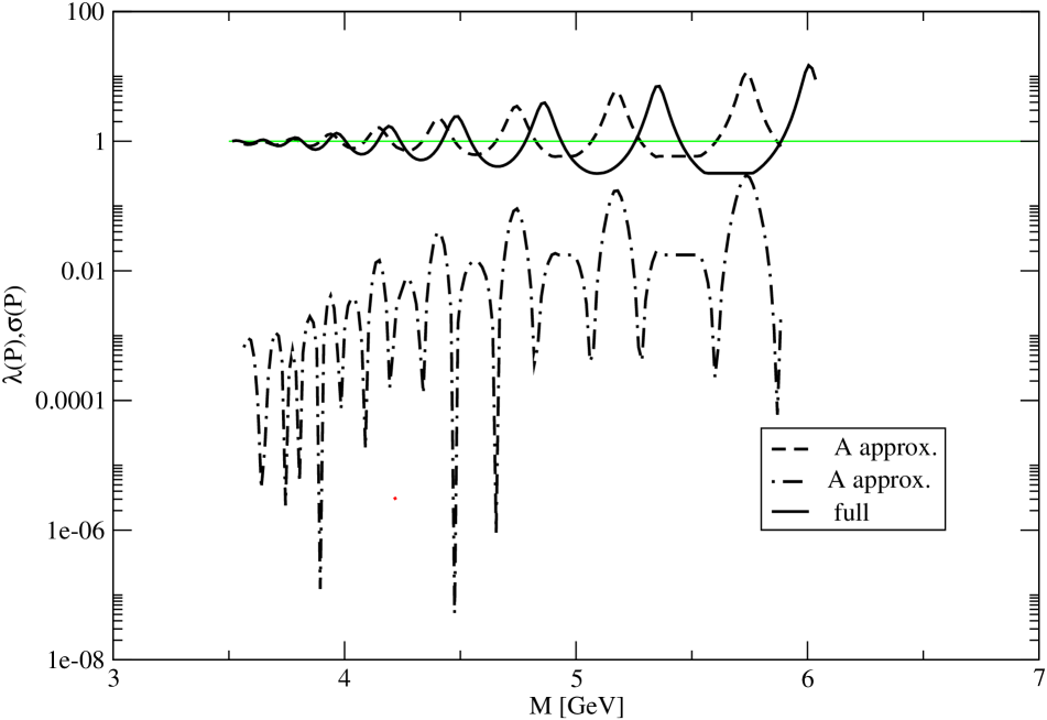
Figure 7: Numerical search for $m_{c}=1.5GeV,\kappa=2.5GeV^{2},\alpha_{s}=0.08,\mu_{v}=\mu_{s}=350MeV$ (solid line). Dashed (dot-dashed) line represents $\lambda,(\sigma)$ in the approximation when only $A$ vertex function has been considered, in this case $m_{c}=1.5GeV,\kappa=2.5GeV^{2},\alpha_{s}=0.0815,\mu_{v}=\mu_{s}=350MeV$.

References

- (1) Quigg C, J.L. Rosner, Phys. Lett. B71, 153 (1977).
- (2) E.Eichten, H. Mahlke, J.L. Rosner, Rev. Mod. Phys. 80, 1161 (2008).
- (3) G. Bonvicini et al. [CLEO Collaboration], Phys. Rev. D 70, 032001 (2004) [arXiv:hep-ex/0404021].
- (4) E.Eichten, K.Gottfried, T.Kinoshita,J.B. Kogut, K.D. lane and T.M. Yan, Phys. Rev. Lett 34, 369 (1975) [Erratum-ibid. 36, 1276 (1976)].
- (5) E.Eichten, K.Gottfried, T.Kinoshita, K.D. Lane and T.M. Yan, Phys. Rev. D 21, 203 (1980)
- (6) B. Aubert et al. [BABAR Collaboration], Phys. Rev. Lett. 101, 071801 (2008) [Erratum-ibid. 102, 029901 (2009)] [arXiv:0807.1086 [hep-ex]].
- (7) R. Alkofer, S. Ahlig, Annals Phys. 275, 113 (1999). ,arXiv:hep-th/9810241v2.
- (8) K. Abe, et al., Phys. ReV. Lett. 98, 082001.
- (9) S.J. Stainsby and R.T. Cahill, Phys. Lett. A146, 467 (1990).
- (10) V. Sauli, Phys. Rev. D 86, 096004 (2012), [arXiv:1112.1865].
- (11) K.G.Wilson, phys.Rev. D 10, 2445 (1974).
- (12) E.Eichten, K.Gottfried, T.Kinoshita,K.D. Lane and T.M. Yan, Phys. Rev. D 17, 3090 (1978) [Erratum-ibid. D21,313 (1980)].
- (13) Takumi Iritani and Hideo Suganuma, Phys. Rev. D83, 054502 (2011).
- (14) Y.B. Ding, K.T. Chao and D.H. Qin, Phys. Rev. D 51, 5064 (1995).
- (15) B.-Q. Li and K.-T. Chao, Phys. Rev. D 79, 094004 (2009).
- (16) Z.Y. Zhang, Y.W. Yu,P.N. Shen,X.Y.Shen, Y.B. Dong, Nucl. Phys. A 261, 595 (1993).
- (17) K.T.Chao and J.H. Liu, in Proceedings of the Workshop on Weak Interactions and CP violations, Beijing, August22-26,1989 World Scientific, Singapore (1990)
- (18) B-Q. Li, K.-T. Chao, Commun. Theor. Phys. 52, 653 (2009).
- (19) P.Gonzales, V. Mathieu, V.Vento, Phys. Rev. D84, 114008 (2011).
- (20) T. Appelquist, R.M. Barnett and K.D. Lane, Ann. Rev. Nucl. Part. Sci. 28, 387 (1987).
- (21) V.A. Novikov,L.B. Okun, M.A. Shifman, A.I. Vainshtein, M.B. Voloshin and V.I. Zakharov, Phys. Rept. 41, 1 1978.
- (22) W. Kwong, C. Quigg and J.L. Rosner, Ann. Rev. Nucl. Part. Sci. 37, 325 (1987).
- (23) N. Brambilla, et all (Quarkonium Working Group) (2004), [arXiv:hep-ph/0412158]
- (24) N. Brambila et al., Eur. Phys. J. C71, 1534 (2011).
- (25) A. C. Aguilar, D. Binosi, J. Papavassiliou, Phys. Phys. Rev. D84, 085026 (2011).
- (26) D. Binosi, J. Papavassiliou, Phys. Rep. 479, (2009).
- (27) A. Cucchieri and T. Mendes, Phys. Rev. D81, 016005 (2010).
- (28) P. Maris, Phys. Rev. D52, 6087 (1995).
- (29) M. Stingl, Phys. Rev. D34 (1986) 3863 [Erratum-ibid. D36 (1987) 651].
- (30) M. Stingl, Z.Phys. A 353 (1996) 423.
- (31) D. Dudal, J.A. Gracey, S.P. Sorella, N. Vandersickel and H.Verschelde, Phys. Rev. D 78, 065047 (2008).
- (32) D. Dudal, O. Oliveira and N. Vandersickel, Phys. Rev. D 81, 074505 (2010).
- (33) A. Cucchieri and T. Mendes, Phys. Rev. Lett. 100, 241601 (2008).
- (34) A. Cucchieri, D. Dudal, T. Mendes, N. Vandersickel, Phys. Rev. D 85, 094513 (2012).
- (35) I. C. Cloet and C. D. Roberts , Prog. Part. Nucl. Phys. 77, 1 (2014).
- (36) Eef van Beveren, George Rupp, arXiv:1005.3490.
- (37) S. J. Brodsky, R. Shrock, Phys. Lett. B 666, 95 (2008).
- (38) V. Sauli, arXiv:1312.2796.