Training Optimization for Energy Harvesting Communication Systems

Abstract

Energy harvesting (EH) has recently emerged as an effective way to solve the lifetime challenge of wireless sensor networks, as it can continuously harvest energy from the environment. Unfortunately, it is challenging to guarantee a satisfactory short-term performance in EH communication systems because the harvested energy is sporadic. In this paper, we consider the channel training optimization problem in EH communication systems, i.e., how to obtain accurate channel state information to improve the communication performance. In contrast to conventional communication systems, the optimization of the training power and training period in EH communication systems is a coupled problem, which makes such optimization very challenging. We shall formulate the optimal training design problem for EH communication systems, and propose two solutions that adaptively adjust the training period and power based on either the instantaneous energy profile or the average energy harvesting rate. Numerical and simulation results will show that training optimization is important in EH communication systems. In particular, it will be shown that for short block lengths, training optimization is critical. In contrast, for long block lengths, the optimal training period is not too sensitive to the value of the block length nor to the energy profile. Therefore, a properly selected fixed training period value can be used.

I Introduction

In traditional wireless sensor networks, the limited energy at each node constrains the network lifetime. Energy harvesting (EH) is a promising technology which has the potential to provide a powerful solution to achieve perpetual lifetime without requiring external power cables or periodic battery replacement [1]. Energy harvesting nodes can harvest energy from the environment, including solar energy, vibration energy, thermoelectric energy, RF energy, etc. With its highly self-reliance capability, EH will undoubtedly play an important role in future green communication networks.

However, employing energy harvesting nodes poses new challenges related to the link and network design, as the harvested energy is typically small and random. Thus although EH technology improves the long-term performance, the challenging short-term performance needs to be guaranteed. Previous works on EH networks have developed communication protocols to either maximize the throughput or minimize the transmission completion time, assuming perfect channel state information (CSI) at the transmitter and receiver, e.g., [2, 3, 4]. In [3], a directional water-filling (DWF) algorithm is proposed to solve the transmit power allocation problem in EH systems, while in [4], a generalized DWF algorithm is proposed to solve a general utility maximization problem.

In a wireless communication link, CSI is important, e.g., for the receiver to decode the transmitted message, or for rate adaptation at the transmitter. At the receiver side, CSI can be obtained by sending pilot symbols from the transmitter. There exists a tradeoff between the training overhead and the training performance. Specifically, spending too much energy or time on channel training will reduce the energy or time for data transmission. On the other hand, training with too little energy or time will degrade the estimation performance. To maximize the throughput, the training period and training power should be carefully selected. Previous studies have shown that in conventional communication systems, training power optimization and training period optimization are decoupled, of which the power optimization is more important. In [5], it was shown that for a point-to-point link without the peak power constraint, the optimal training policy involves sending one pilot symbol with optimized training power. However, in EH communication systems, the training design is different and is largely influenced by the low rate and randomness property of the available energy. The selection of the training period and training power in EH systems are coupled and both will depend on the EH profile in the communication block. Therefore, the training design in EH communication systems is more challenging and plays a more important role.

In this paper, we investigate the training optimization problem in EH communication systems. We first characterize the properties of the training design in an EH communication system. We then propose two different training policies to determine the training period and power. The first training policy adaptively adjusts the training period based on the energy profile in the whole transmission block, while the second one is designed in an adaptive way according to the average EH rate of the block. Simulation results will show that training optimization is important to improve the communication performance in EH systems, especially when the transmission block is not very long. For long block lengths, the optimal training period is not too sensitive to the value of the block length. Therefore, a fixed training period value can be used if properly selected.

II System Model

We consider a point-to-point communication link where the transmitter is an EH node, as shown in Figure 1. The transmitter can only use the energy it harvests, and we assume that all the harvested energy is used for communication. The channel is characterized by block fading, and within a coherence block, the channel gain $h$ is constant with $h\sim\textrm{CN}\left(0,\sigma_{h}^{2}\right)$. The additive white Gaussian noise is denoted as $n$ with $n\sim\textrm{CN}\left(0,\sigma^{2}\right)$. The communication within one transmission block includes two stages: the training stage and the data transmission stage. The partition of the two stages is in the unit of a time slot $T_{S}$. The fading block length is denoted as $T$, with $N=\frac{T}{T_{S}}$ slots, while the training stage length is $T_{t}$, with $N_{t}=\frac{T_{t}}{T_{S}}$ slots. During the training stage, the receiver obtains an estimate of $h$, denoted as $\hat{h}$, through the use of a pilot signal. The estimation error is denoted as $\tilde{h}$ with $\tilde{h}=h-\hat{h}$. Before the transmission stage, the receiver feeds back the value of $\hat{h}$ to the transmitter. The feedback channel is assumed to be perfect, while the case with unideal feedback will be discussed in future work.

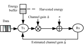
Figure 1: The basic system model.

II-A Energy Model

An important factor that determines the performance of an EH system is the EH profile, which models the variation of the harvested energy with time. Several different types of EH profiles are shown in the left part of Figure 2. For convenience, we plot all EH profiles inside a 2-D coordinate system of accumulated energy versus time.

To demonstrate the property and impact of energy profiles, we adopt similar EH assumptions as in [2, 3]. Specifically, we assume that the energy profile in the considered transmission block is known before the communication starts. This assumption is applicable for predictable energy models, such as solar energy [6].

The utilization of the harvested energy is constrained by the EH profile, and therefore the energy neutrality constraint exists in EH systems [7]. The energy neutrality means that the energy consumed thus far cannot exceed the total energy harvested. For simplicity, we assume that the EH node can only use the energy harvested in the previous slots. If the consumed power is denoted as $P\left(t\right)$, the initial energy in the energy buffer as $E_{0}$, and the harvested energy in the $k$th slot as $E_{k}$, then the energy neutrality constraints can be expressed as

$$\int_{0}^{l{T_{S}}}{P}\left(t\right)dt\leq\sum_{k=0}^{l-1}E_{k},$$ (1)

where $l$ is the index of the time slot with $l=1,2,...,N$.

As shown in (1), a certain EH profile determines a feasible energy consumption domain, and only the policies inside this domain are feasible energy consumption policies, both of which are plotted in the same coordinate system with the EH profile in the right part of Figure 2. Due to the energy neutrality constraint (1), we cannot use the energy arriving in the future, but can back up the current energy for future use. This causal energy constraint determines the directional property of all power allocation policies in EH systems, which will be discussed in more detail later.

Among all kinds of EH processes, there are two special cases: the non-EH case and the constant-rate EH case, as shown in the left part of Figure 2. Here we treat the conventional non-EH system, i.e., without the EH function and only with the average power constraint, as an extreme case of energy harvesting, in which all the energy arrives before the first slot. This is equivalent to relaxing all the causal energy constraints. The feasible energy domain of non-EH nodes is the union of all the possible EH profiles with the same total energy in a given time duration, so it provides the best performance among all the EH profiles. Constant-rate EH refers to the node that can harvest energy at a constant rate. In this case, the profile can be considered as a deterministic process. In practical systems, when the EH profile does not change frequently or the block length is small, a constant-rate EH profile is a good approximation of the energy profile in each transmission block, with the mean of the EH process as its harvesting rate.

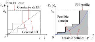
Figure 2: The energy profile and feasible energy consumption policies in the 2-D coordinate system of accumulated energy versus time. The left part plots energy profiles, for two general EH cases, and two special cases: the non-EH case and the constant-rate EH case. The right part plots the feasible energy consumption domain and policies for a given EH profile, of which the bold line is the EH profile, the area under it is the feasible domain, and a curve connecting the bottom-left point and the top-right point inside this domain is a feasible energy consumption policy, two examples of which are shown.

The battery capacity is also an important factor for the EH link performance besides the EH profile. In this paper we assume that the energy buffer is of an infinite capacity, while the case with a finite buffer capacity will be dealt with in future work.

III Impact of Channel Training in EH systems

In this section, we first investigate the training policy for EH systems and compare it with non-EH systems. We will then develop power allocation for the data transmission stage.

III-A Training Stage in EH Systems

In the training stage, we denote the average training power in the $j$th time slot as $\bar{P_{j}}$ $\left(1\leq j\leq N_{t}\right)$, then the variance of the estimation error with an MMSE channel estimator is [8]

$$\sigma_{\tilde{h}}^{2}=\frac{\sigma^{2}\sigma_{h}^{2}}{\sigma^{2}+\sigma_{h}^{2}\sum_{j=1}^{N_{t}}\bar{P_{j}}}.$$ (2)

We see that only the sum of average training powers matters. This means that as long as the total training power is the same, the training performance is fully determined, independent of the training period or the power allocation inside this stage. Thus, we will use the discrete-time expression of $P_{j}=\bar{P_{j}}$ to denote training powers.

Due to the causal energy constraint in EH systems, there exists a big difference in the training design for non-EH systems and EH systems. In the non-EH system without a peak power constraint, the optimal $N_{t}$ is always 1 [5], as shown in the left part of Figure 3. An intuitive explanation is that we can always achieve a good training performance with enough training power (as long as it is less than the total power available). Meanwhile, we shall make the training period as small as one time slot. Thus, what matters is the power allocated for channel training rather than the training period. However, this is not the case for the EH system. Due to the stochastic EH profile, the energy arrival in the first time slot may be very small, as shown in the right part of Figure 3. Hence, fixing the training period as 1 slot will generally provide an inaccurate channel estimation. The total training power is largely determined by the training period, which makes it more important than the power allocation, and increases the difficulty of the training design.

In EH systems, we select such a training power allocation policy that, for a given $N_{t}$, all the harvested energy for $1\leq j\leq N_{t}-1$ is exhausted, while there may be some energy left at slot $N_{t}$, of which the value is optimized. This is optimal because it is not possible to find a smaller training period $N_{t}^{\prime}<N_{t}$ to achieve the same training performance.

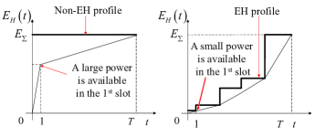
Figure 3: Comparison of the power allocation policies in the training stage for non-EH and EH systems. The left and right figures represent the non-EH and EH cases, respectively.

III-B Data Transmission Stage in EH Systems with Estimation Errors

Considering the channel estimation error and the training overhead, the average achievable throughput in each time slot is

$$R=\textrm{E}_{\hat{h}}\left[\frac{1}{N}\sum_{i=N_{t}+1}^{N}\log_{2}\left(1+\frac{\left|\hat{h}\right|^{2}P_{i}}{\sigma^{2}+P_{i}\sigma_{\tilde{h}}^{2}}\right)\right].$$ (3)

As shown in [9], this is a lower bound for the capacity with channel estimation error and we will use it as the performance metric in the paper.

By substituting (3) and adopting (9) in [10], this rate expression can be finally transformed to

$$R=\frac{1}{N}\log_{2}\left(e\right)\sum_{i=N_{t}+1}^{N}\exp\left(\frac{1}{K_{i}}\right)\textrm{E}_{1}\left(\frac{1}{K_{i}}\right),$$ (4)

where $K_{i}=\frac{\sigma_{h}^{4}P_{i}\sum_{j=1}^{N_{t}}P_{j}}{\sigma^{4}+\sigma^{2}\sigma_{h}^{2}P_{i}+\sigma^{2}\sigma_{h}^{2}\sum_{j=1}^{N_{t}}P_{j}}$, and $\textrm{E}_{1}\left(x\right)=\int_{x}^{+\infty}t^{-1}e^{-t}dt$.

Different from non-EH systems that use a constant transmit power in the data transmission stage, in the EH system, we need to determine the power allocation between different time slots, as the power allocated to each slot needs to satisfy the energy neutrality constraint (1). For given $N_{t}$, $\hat{h}$ and $\sigma_{\tilde{h}}^{2}$, the power allocation problem is as follows:

Problem 1:

$$\begin{array}[]{cl}\max\limits_{P_{N_{t}+1},...P_{N}}&\frac{1}{N}\sum_{i=N_{t}+1}^{N}\log_{2}\left(1+\frac{\left|\hat{h}\right|^{2}P_{i}}{\sigma^{2}+P_{i}\sigma_{\tilde{h}}^{2}}\right)\\ {\rm{s}}.{\rm{t}}.&{T_{S}}\sum\limits_{i=N_{t}+1}^{l}{P_{i}}\leq E_{te}+\sum_{k=N_{t}}^{l-1}E_{k}\\ &{T_{S}}\sum\limits_{i=N_{t}+1}^{N}{P_{i}}=E_{te}+\sum_{k=N_{t}}^{N-1}E_{k}\\ &l=N_{t}+1,...,N-1,\end{array}$$

where $E_{te}$ denotes the energy left from the training operation, and is known before the optimization.

In Problem 1, the first constraint is the energy neutrality constraint. In contrast to non-EH systems, even if the channel stays unchanged, the power still needs to be adaptively allocated from slot to slot due to the causal EH constraints. The second constraint means that at the end of the block, the node needs to use up all the available energy, as we do not consider the energy sharing between blocks to render our problem tractable, while the case with block-to-block energy sharing will be discussed in future work.

We make the following two comments on Problem 1. First, similar to the training power, the data transmission power is expressed in a discrete-time form, as it is optimal for the power inside one slot to be constant due to the concavity of the objective function. Second, as the training power and the data transmission power are the same from the perspective of energy consumption, we use the same notation $P$ and only distinguish between them by the time index.

The throughput expression with estimation errors satisfies the condition of the directional water-filling (DWF) algorithm [4], and thus the optimal power allocation follows DWF. Such a DWF algorithm has a special property that the solution is only determined by constraints, irrespective of the parameters in the objective function. So in our problem the solution is independent of $\hat{h}$ and $\sigma_{\tilde{h}}^{2}$, i.e., the estimation performance and the value of the estimated channel gain do not have any impact on the power allocation. This special property can largely simplify the power allocation, as there is no need to completely reallocate the data transmission power for different values of $N_{t}$. We only need to execute the power allocation over the whole block once for $N_{t}=0$, and update a few points for other values of $N_{t}$. Accordingly, we develop an efficient algorithm to solve Problem 1 for different $N_{t}$, as shown in Algorithm 1.

1. Initialization: Set integers $k_{0}=0$ and $n=1$.

2. Iteration: Iterate $k_{n}=\arg\underset{k:k\leq N}{\min}\left\{\frac{\sum_{j=k_{n-1}}^{k-1}E_{j}}{k-k_{n-1}}\right\}$ with $n$ adding 1 each time, until $k{}_{n}=N$, so finally an index set $\mathcal{K}_{0}=\left\{k_{n}\right\}$ is constructed.

3. Results for $N_{t}$=0: The optimal power in the $i$th slot is $p_{n}=\frac{\sum_{j=k_{n-1}}^{k_{n}-1}E_{j}}{k_{n}-k_{n-1}}$ for $i\in\left[k_{n-1}+1,k_{n}\right]$, and a power set $\mathcal{P}_{0}=\left\{p_{n}\right\}$ is obtained for $N_{t}$=0.

4. Update for $N_{t}\neq 0$: Reset $k^{\prime}_{0}=N_{t}$, recalculate $k^{\prime}_{1}=\arg\underset{k:k\leq N}{\min}\left\{\frac{\sum_{j=k^{\prime}_{0}}^{k-1}E_{j}}{k-k^{\prime}_{0}}\right\}$, then the index set for $N_{t}$ is $\mathcal{K}_{N_{t}}=\left\{k^{\prime}_{1}\right\}\cup\left\{\textrm{all }k_{n}\in\mathcal{K}_{0}\textrm{ that }k_{n}>k^{\prime}_{1}\right\}$.

5. Results for $N_{t}\neq 0$: The power for $i\in\left[k_{0}+1,k^{\prime}_{1}\right]$ is $p^{\prime}_{1}=\frac{\sum_{j=k^{\prime}_{0}}^{k^{\prime}_{1}-1}E_{j}}{k^{\prime}_{1}-k^{\prime}_{0}}$, while the other powers are unchanged, then the power set for $N_{t}$ is $\mathcal{P}_{N_{t}}=\left\{p^{\prime}_{1}\right\}\cup\left\{\textrm{all }p_{n}\in\mathcal{P}_{0}\textrm{ that }p_{n}>p^{\prime}_{1}\right\}$.

Algorithm 1 DWF algorithm for Problem 1 with different $N_{t}$

From Algorithm 1, we can see that for a given $N_{t}$, the power allocation result consists of several intervals, and the power is a constant value inside each of these intervals. The endpoint indices of all intervals form an index set $\mathcal{K}_{N_{t}}$, while the powers in these intervals form a power allocation set $\mathcal{P}_{N_{t}}$. Furthermore, according to Steps 4 and 5 of Algorithm 1, for different $N_{t}$, the majority ($i\in\left[k^{\prime}_{1},N\right]$) of the transmit power allocation is unvaried, while only a small proportion ($i\in\left[k_{0}+1,k^{\prime}_{1}\right]$) changes with $N_{t}$. This property brings the possibility of decoupling the training power allocation and the selection of training period, which will be used in the next section for the optimal training design.

IV Optimal Training Design

As seen from the last section, in EH communication systems, the coupling of the training period selection and the training power allocation brings the main difficulty in the training design, and the training period selection is especially critical. In this section, we will investigate the optimal training design in EH systems and propose two training policies.

IV-A Problem Formulation

With the average throughput in (4) as the objective and considering energy neutrality constraints, the optimal training problem in EH communication systems is formulated as

Problem 2:

$$\begin{array}[]{cl}\max\limits_{P_{1},...P_{N},N_{t}}&\sum\limits_{i=N_{t}+1}^{N}{\exp}\left({\frac{1}{{K_{i}}}}\right){{\rm{E}}_{1}}\left({\frac{1}{{K_{i}}}}\right)\\ {\rm{s}}.{\rm{t}}.&1\leq{N_{t}}<N,\begin{array}[]{c}\end{array}N_{t}\in\mathbb{N}\\ &{T_{S}}\sum\limits_{i=1}^{l}{P_{i}}\leq\sum_{k=0}^{l-1}E_{k},\begin{array}[]{c}\end{array}l=1,2,...,N-1\\ &{T_{S}}\sum\limits_{i=1}^{N}{P_{i}}=\sum_{k=0}^{N-1}E_{k}.\end{array}$$

This problem has two difficulties: 1) the optimization of $N_{t}$ and $P_{i}$ are coupled; 2) the optimization variable $N_{t}$ exists in the summation limit in the objective function, and only takes discrete values. Due to the intractability of this problem, we propose a sub-optimal solution in the next subsection.

IV-B A Sub-optimal Solution

Due to the difficulties of Problem 2, we adopt a DWF approximation and a rate approximation to derive a sub-optimal solution. Both of these simplifications have good approximation properties, which will be verified by the simulation results. In addition, for the special case of the constant-rate EH, both approximations become equivalent to the original problem. As commented in Section II, the constant-rate EH model is a good approximation for the energy profile in each transmission block in different EH systems, so our sub-optimal solution will be in general close to optimal.

IV-B1 DWF Approximation

First, based on the property of Algorithm 1 as discussed in Section III.B, we make an approximation to decouple the training power allocation and the training period selection. From Algorithm 1, the power allocation in the whole transmission block only changes in a small number of slots for different values of $N_{t}$. We make an approximation that the power allocation is fixed for all values of $N_{t}$, i.e., we ignore the possible changes of power allocation in some slots for different $N_{t}$. This simplification will decouple $N_{t}$ and $P_{i}$, so that we can perform the DWF power allocation just once, and then optimize $N_{t}$ over a fixed power allocation result. In this way, we can get a sub-optimal solution with low computational complexity.

IV-B2 Rate Approximation

With the DWF approximation, the problem is still intractable, as the variable $N_{t}$ only takes integer values and appears in the summation of the objective function. To further simplify the problem, we make the following rate approximation: first, for a given value of $N_{t}$, we calculate the estimation error assuming a constant training power to equal the average EH rate $\bar{P}_{H}$, i.e., $\sigma_{\tilde{h}}^{2}=\frac{\sigma^{2}\sigma_{h}^{2}}{\sigma^{2}+\sigma_{h}^{2}\sum_{j=1}^{N_{t}}P_{j}}\approxeq\frac{\sigma^{2}\sigma_{h}^{2}}{\sigma^{2}+\sigma_{h}^{2}N_{t}\bar{P}_{H}}$; second, we determine the achievable throughput $\hat{R}$ assuming all the slots including the training period are used for data transmission with the transmit power equal to the DWF result in the respective slot, i.e., $\hat{R}=\sum_{i=1}^{N}M_{i}$, where $M_{i}=\exp\left(\frac{1}{K_{i}}\right)\textrm{E}_{1}\left(\frac{1}{K_{i}}\right)$ is the average throughput for the $i$th slot considering the estimation error; finally, we include the throughput loss due to the training period, i.e., $R=\sum_{i=N_{t}+1}^{N}M_{i}\approxeq\frac{N-N_{t}}{N}\sum_{i=1}^{N}M_{i}=\frac{N-N_{t}}{N}\hat{R}$. To summarize, Step 1 is to consider the effect of the estimation error, Step 2 is adopting the DWF approximation while ignoring the time taken by training, and Step 3 is to take the time consumed by training back into consideration. While greatly simplifying the problem, this rate approximation preserves the essential tradeoff in the original training design problem, i.e., the tradeoff between the resource consumed by training and the estimation performance.

IV-B3 Solution to the Simplified Problem

Based on previous two steps, the training design problem can be formulated as:

Problem 3:

$$\begin{array}[]{ll}\underset{{}_{N_{T}}}{\max}&\frac{N-N_{t}}{N}\sum_{i=1}^{N}\exp\left(\frac{1}{K_{Si}}\right)\textrm{E}_{1}\left(\frac{1}{K_{Si}}\right)\\ {\rm{s}}.{\rm{t}}.&1\leq{N_{t}}<N,\begin{array}[]{c}\end{array}N_{t}\in\mathbb{N},\end{array}$$

where $K_{Si}=\frac{\sigma_{h}^{4}P_{i}N_{t}\bar{P}_{H}}{\sigma^{4}+\sigma^{2}\sigma_{h}^{2}P_{i}+\sigma^{2}\sigma_{h}^{2}N_{t}\bar{P}_{H}}$, and all $P_{i}$ are determined through Step 1~3 of Algorithm 1. The solution for Problem 3 is a sub-optimal solution for Problem 2.

For simplicity, we denote $x=\frac{1}{N_{t}}$. When $x$ is assumed continuous, the objective function is concave, the proof of which is omitted due to space limitation. Through the derivative with respect to $x$ we can get an implicit solution, i.e., the solution of Problem 3 is the solution of the following equation (the discretization part is omitted due to space limitation)

$$\sum_{i=1}^{N}\left\{M_{i}\left[1+\left(\frac{N}{N_{t}}-1\right)\frac{\sigma^{2}}{\sigma_{h}^{2}P_{i}G_{i}}\right]-\frac{\left(\frac{N}{N_{t}}-1\right)}{1+G_{i}}\right\}=0,$$ (5)

where $G_{i}=\frac{\sigma_{h}^{2}\bar{P}_{H}N_{t}}{\sigma^{2}+\sigma_{h}^{2}P_{i}}$.

When $N$ approaches infinity, we can get an asymptotic solution of $N_{t}$ and its ratio over $N$ in closed form as

$$N_{t}=\frac{2N}{1+\sqrt{1+4NW}},\begin{array}[]{c}\end{array}\,\begin{array}[]{c}\end{array}\,\begin{array}[]{c}\end{array}\,\begin{array}[]{c}\end{array}\,\alpha=\frac{N_{t}}{N}=\frac{2}{1+\sqrt{1+4NW}},$$ (6)

where $W=\frac{\sum_{i=1}^{N}M_{i}^{A}}{\sum_{i=1}^{N}\frac{\sigma^{4}+\sigma^{2}\sigma_{h}^{2}P_{i}}{\sigma^{2}\sigma_{h}^{2}\bar{P}_{H}}\left(1-\frac{\sigma^{2}M_{i}^{A}}{\sigma_{h}^{2}P_{i}}\right)}$, and $M_{i}^{A}=\exp\left(\frac{\sigma^{2}}{\sigma_{h}^{2}P_{i}}\right)\textrm{E}_{1}\left(\frac{\sigma^{2}}{\sigma_{h}^{2}P_{i}}\right)$.

From the expression of solution (6), we see that the optimal training period is influenced by the block length and EH profiles. Generally speaking, a larger block length will result in a longer training period $N_{t}$, but a smaller training period ratio $\alpha=\frac{N_{t}}{N}$. When $N$ approaches infinity, $N_{t}$ also approaches infinity, while the ratio $\alpha$ approaches zero.

IV-C A Special Case – The Constant-rate EH Profile

The constant-rate EH process can be used to approximate any general EH system when the energy harvesting rate does not change intensively. Thus, in this section we will show that the optimal solution of the constant-rate EH case can provide another sub-optimal solution for the general EH systems with the same average EH rate. This solution is very practical as it only needs the mean value of the EH profile, rather than its instantaneous realization.

To optimize $N_{t}$ for the constant-rate EH case, the gradient analysis of throughput shows that the optimal value for both the training and transmission powers equals the EH rate, denoted by $P_{H}$, i.e., the transmit power is a constant in both stages, and we only need to determine $N_{t}$, the training period.

By applying (5) to the constant-rate EH case, the optimal $N_{t}$ for the constant-rate EH is the solution of

$$M^{Con}\left[1+\left(\frac{N}{N_{t}}-1\right)\frac{\sigma^{2}}{\sigma_{h}^{2}P_{H}G{}^{Con}}\right]-\frac{\left(\frac{N}{N_{t}}-1\right)}{1+G^{Con}}=0,$$ (7)

where $G^{Con}=\frac{\sigma_{h}^{2}P_{H}N_{t}}{\sigma^{2}+\sigma_{h}^{2}P_{H}}$, $M^{Con}=\exp\left(\frac{1}{K^{Con}}\right)\textrm{E}_{1}\left(\frac{1}{K^{Con}}\right)$, and $K^{Con}=\frac{\sigma_{h}^{4}P_{H}^{2}N_{t}}{\sigma^{4}+\sigma^{2}\sigma_{h}^{2}P_{H}\left(1+N_{t}\right)}$.

Note that (7) is the exact optimal solution for a constant-rate EH system. Meanwhile, it also provides an approximate solution for a general EH communication system. Thus, we propose a second sub-optimal solution to Problem 2 as follows. First, we equate the total energy in a given transmission block of a general EH system with that of a constant-rate EH system, from which we can get an equivalent $\hat{P}_{H}$, the average EH rate. Then, the approximate solution is derived by solving the training optimization problem for a constant-rate EH system with rate $\hat{P}_{H}$. This provides a sub-optimal value of $N_{t}$. Once we get this value of $N_{t}$, the directional water-filling algorithm can be applied for power allocation in the data transmission stage to further improve the performance.

V Simulation Results

In this section, we provide simulation results to show the importance of training optimization in EH communication systems. We will compare the throughput performances of the optimal policy, two sub-optimal policies, and several fixed training policies. The result of the optimal policy, i.e., the solution of Problem 2, is obtained by exhaustive search. The sub-optimal solutions include (5) as sub-optimal solution 1, and (7) as sub-optimal solution 2. The fixed training policies include: fixing a training period value $N_{t}$, fixing the training period ratio $\frac{N_{t}}{N}$, and the conventional fixing 1-slot policy, i.e., $N_{t}=1$. These training policies will also be compared with two performance upper bounds. One upper bound assumes perfect CSI and with the same EH process. It will be denoted as “upper bound 1”. The second is the non-EH case with the same total energy in each transmission block and adopting the optimal channel training in [5]. We shall denote it as “upper bound 2”.

In the simulation, we assume that the channel is distributed as $h\thicksim\textrm{CN$\left(0,1\right)$}$. Both the energy arrival process in each time slot and the initial energy in the energy buffer are assumed to be Poisson distributed, with parameter $\lambda_{e}$ set to be 1. The average SNR is also 1.The simulation is run for 1000 random EH realizations. We select $N_{t}=30$ for the fixed training period scheme, and $N_{t}=0.04N$ for the fixed training period ratio scheme. The results are shown in Figure 4.

We see that the optimal policy and two sub-optimal policies are very close to each other, and all have small gaps to the performance bounds. The achievable throughput of sub-optimal solution 2 is slightly lower than that of sub-optimal solution 1. It should be emphasized that the sub-optimal solution 2 does not need the instantaneous realization of the EH process, but only the average energy harvesting rate of the process, which makes it more practical. We can also find that when $N$ is small, the gaps between all the fixed policies and the optimal one are very large, which means that we need to adaptively adjust the training period for different EH profiles. However, when $N$ is large, the throughput gaps between the fixed policies and the optimal one are not very big, except for $N_{t}=1$. This means that in a low mobility environment, i.e., with a large $N$, it is feasible to select a fixed training period or ratio not only independent of the EH process, but also independent of the block length.

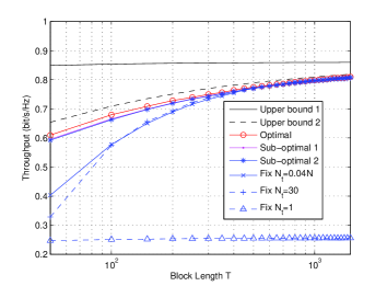
Figure 4: The comparison of different training schemes for various block lengths assuming a Poisson EH process.

Next, we elaborate more on the fixed $N_{t}$ policy, as we cannot change $N_{t}$ in some practical systems. Considering typical values of coherence bandwidth $W_{c}=500\textrm{kHz}$ and coherence time $T_{c}=2.5\textrm{ms}$ (from [11]) as an example, the block length is $N=1250$. Figure 5 compares the throughput of the optimal policy with adaptively selected $N_{t}$ and the fixed policy with different fixed values of $N_{t}$. We can see that when $N_{t}$ lies in the interval $\left[13,128\right]$, the performance gap between the fixed policy and optimal policy is within $5\%$; while the interval for a $10\%$ gap is $\left[8,189\right]$. This indicates that as long as $N_{t}$ belongs to a proper region, it is a fairly good policy to fix $N_{t}$ independent of the instantaneous EH process.

From these results, we see that if the training period can be adaptively adjusted in each block, we can get the approximate optimal value using the sub-optimal solution 2 in (7). On the other hand, if the training period needs to be fixed, we can select a proper fixed value according to the throughput gap requirement, which will work well especially for the low mobility environment.

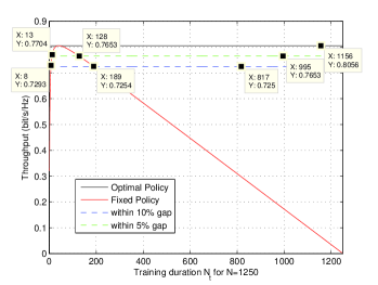
Figure 5: Performance of the optimal policy and the fixed policy for $N$ = 1250 with a Poisson EH process. The optimal policy adaptively picks a value of $N_{t}$ for different energy profiles, while the fixed policy always chooses a single $N_{t}$.

VI Conclusions

In this paper, we investigated the optimal training design for EH communication systems, which was shown to be quite different from conventional non-EH systems and poses new challenges. We found that the training period should be carefully selected, especially when the coherence block length is not very long. In particular, we proposed two sub-optimal training policies to determine the training period and power, the second of which is especially attractive as it only requires information about the average EH rate instead of the detailed energy profile in each transmission block. Furthermore, we demonstrated that in low mobility environments, a carefully selected fixed training period can provide satisfactory performance, which provides a practical option for systems that cannot adaptively adjust the training period.

References

- [1] J. Paradiso and T. Starner, “Energy scavenging for mobile and wireless electronics,” IEEE Pervasive Comput., vol. 4, pp. 18–27, Jan.–Mar. 2005.
- [2] J. Yang, and S. Ulukus, "Optimal packet scheduling in an energy harvesting communication system," IEEE Trans. Commun., vol. 60, no.1, pp.220-230, Jan. 2012.
- [3] O. Ozel, K. Tutuncuoglu, J. Yang, S. Ulukus, and A. Yener, “Transmission with energy harvesting nodes in fading wireless channels: optimal policies,” IEEE J. Select. Areas Commun., vol. 29, no. 8, pp. 1732 –1743, Sep. 2011.
- [4] K. Tutuncuoglu and A. Yener, “Communicating with energy harvesting transmitters and receivers,” in Proceedings of 2012 Information Theory and Applications Workshop, ITA, San Diego, CA, Feb 2012.
- [5] M. C. Gursoy, “On the capacity and energy efficiency of training-based transmissions over fading channels,” IEEE Trans. Inf. Theory, vol. 55, pp. 4543–4567, Oct. 2009.
- [6] M. Gorlatova, A. Wallwater, and G. Zussman, "Networking low-power energy harvesting devices: measurements and algorithms," Proc. IEEE INFOCOM, Apr. 2011.
- [7] A. Kansal, J. Hsu, S. Zahedi, and M. B. Srivastava, “Power management in energy harvesting sensor networks,” ACM Trans. Embed. Comput. Syst., vol. 6, Sep. 2007.
- [8] Steven M. Kay, Fundamentals of Statistical Signal Processing: Estimation Theory. Prentice Hall, 1993.
- [9] M. Medard, “The effect upon channel capacity in wireless communications of perfect and imperfect knowledge of the channel,” IEEE Trans. Inf. Theory, vol. 46, pp. 933-946, May 2000.
- [10] J. Zhang and J. G. Andrews, “Adaptive spatial intercell interference cancellation in multicell wireless networks,” IEEE J. Select. Areas Commun., vol. 28, no. 9, pp. 1455–1468, Dec. 2010.
- [11] D. Tse and P. Viswanath, Fundamentals of Wireless Communication. Cambridge University Press, 2005.