Particle Production in the Field Theories with Symmetry

Abstract

The field theory with high space-time symmetry is considered with the aim to examine the mass-shell particles production processes. The general conclusion is following: no real particle production exists if the space-time symmetry constraints are taken into account. This result does not depend on the concrete structure of Lagrangian.

I Introduction

The purpose of present article is to calculate the cross section of inelastic processes in theories with high space-time symmetry. We will consider a case when the action, $S$, have the nontrivial extremum at $u(x)$,

$$u(x):\frac{dS(\varphi)}{\delta\varphi(x)}=0,$$ (1)

where $\varphi$ is the boson field. The quantitative consideration of this question seems important since although there exists a number of approaches to the canonical quantum field theory formalism in the vicinity of extended field $u(x)\neq 0$, see e.g. goldst ; jakiw , the observables practically were not considered because of the complicated problem with symmetry constraints . A theory in which the consequences of broken by $u(x)$ symmetry is taken into account explicitly will be called as ”the field theory with symmetry” understanding that $u(x)$ is the result, at least, of high space-time symmetry of action $S(\varphi)$.

The main physical result of present paper looks as follows: the transition of interacting field into the mass-shell particles state, and vice versa, is impossible in the field theories with symmetry. We will consider the general case, $u(x)$ is not necessarily the soliton field which is absolutely stable against decay on the particles, see e.g. jakiw . The introduction into the necessary formalism and quantitative prove of $2d$ solitons stability against particles decay was described in the review paper prepr . The main formal result of this work is the further development of formalism prepr ; tmf which is able to solve particle production problem in the $4d$ field theories with symmetry.

It will be shown explicitly at the very end that the $m-$ into $n-$particles transition cross section times a flux factor, $\rho_{mn}$, is trivial:

$$\rho_{mn}=0,~{}~{}\forall(m,n)>0,$$ (2)

if the field theory with symmetry is considered.

In Sec.2 the cross section $\rho_{mn}$ will be introduced and in Sec.3 the method of calculation of $\rho_{mn}$ will be described. The prove of Eq. (2) will be given in Sec.4. A short list of unsolved problem will be given in the last Sec.5.

The conclusion (2) can be extended directly on the gluon production case in non-Abelian gauge theory without matter (quark) fields, see also Sec.5.

II Integral representation for generating functional of $\rho_{mn}$

It will be seen that the used formalism allows to act ex adverso. So, we will introduce $S$-matrix using ordinary LSZ reduction formalism. The conclusion (2) is general, it does not depend on the concrete form of theory Lagrangian, $L$. For this reason one can have in mind the simplest $4d$ conformal scalar field theory:

$$L=\frac{1}{2}(\partial\varphi)^{2}-\frac{g}{4}\varphi^{4},~{}g>0,$$ (3)

as an example to consider massless scalar particles production, see Appendix A where particles production in the theory with Lagrangian (3) is described.

II.1 Generating functional

We expect that the interaction of internal states with external particles is switched on adiabatically, i.e. that the external fields can not have an influence to the spectrum of interacting field perturbations in the case of field theory with symmetry. The builded formalism will correspond to this basic condition.

So, the $(m+n)$-point Green function $G_{mn}$ is defined by a formulae:

$$G_{mn}(y_{1},y_{2},...,y_{m};x_{1},x_{2},...,x_{n})=\int D\varphi\prod_{k=1}^{m}\varphi(y_{k})\prod_{k=1}^{n}\varphi(x_{k})e^{iS(\varphi)}.$$

The LSZ reduction formula means that the external legs (massless particles in the considered case) must be amputated, i.e. the amplitude is defined by the expression caruzerss , see also physrep :

$$A_{mn}(y_{1},...,y_{m};x_{1},...,x_{n})=\int D\varphi\prod_{k=1}^{m}\partial^{2}_{y_{k}}\varphi(y_{k})\prod_{k=1}^{n}\partial^{2}_{x_{k}}\varphi(x_{k})e^{iS(\varphi)},$$

and the amplitude in the energy-momentum representation looks as follows, see Fig.1:

$$a_{mn}(q_{1},....q_{m};p_{1},p_{2},...,p_{n})=\int D\varphi\prod_{k=1}^{m}\Gamma(q_{k};\varphi)\prod_{k=1}^{n}\Gamma^{*}(p_{k};\varphi)e^{iS(\varphi)},$$ (4)

where

$$\Gamma(q;\varphi)=\int dxe^{-ixq}\partial^{2}\varphi(x),~{}q^{2}=0,$$ (5)

is the external particles annihilation vertex. It must be noted absence of the energy-momentum conservation $\delta$-functions in the definition of the amplitude (4). Considering the extended field configurations, $u(x)$, the conservation of the external particles energy and momentum is the isolated problem, see tmf . In considered case this question is not important.

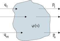
Figure 1: The amplitude $a_{mn}$. The plane wave $e^{-iq_{k}x_{k}}$, $k=1,2,...,m$, is associated to each in-coming particle and $e^{ip_{k}y_{k}}$, $k=1,2,...,n$, to each out-going one. It is supposed that $q_{k}^{2}=p_{k}^{2}=0$. The integration over $\varphi(x)$ must be performed.

The common point of view on the multiple production gives the method of generating functionals, $R(z)$, through the expression:

$$R(z)=\sum_{m,n}\frac{1}{m!n!}\int d\omega_{m}(z,q)d\omega_{n}^{*}(z,p)|a_{mn}(q_{1},...,q_{m};p_{1},...,p_{m})|^{2},$$

see Fig.2, where the usual probe function $z(q)$ was introduced:

$$d\omega_{m}(z,q)=\prod_{k=1}^{m}\frac{d^{3}q_{k}z(q_{k})}{(2\pi)^{3}2\varepsilon(q_{k})},~{}~{}\varepsilon(q)=\sqrt{q^{2}}$$

and $dz/dz^{*}\equiv 0$. As a result,

$$R(z)=\sum_{m,n=0}^{\infty}\frac{1}{m!n!}\int D\varphi^{+}D\varphi^{-}\left\{e^{iS(\varphi^{+})}{N(z,\varphi^{\pm})}^{m}\right\}\left\{e^{-iS^{*}(\varphi^{-})}{N^{*}(z,\varphi^{\pm})}^{n}\right\},$$ (6)

where

$$N(z,\varphi^{\pm})=\int d\omega_{1}(z,q)\Gamma(q;\varphi^{+})\Gamma^{*}(q;\varphi^{-}).$$ (7)

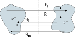
Figure 2: The diagram for $(m+n)$-particle absorption part of vacuum-into-vacuum amplitude. Each in-coming line carry the factor $z(q_{k})$, $k=1,2,...,m$, and $z^{*}(p_{k})$, $k=1,2,...,n$ is associated with out-going one. The field $\varphi_{+}$ is defined on the Mills complex time contour $C^{+}$ and $\varphi_{-}$ is defined on $C^{-}=C^{+*}$ prepr . The summation over $m$ and $n$ and the independent integration over $\varphi_{+}$ and $\varphi_{-}$ must be performed. The vertical dotted line cross mass-shell particle lines

The quantity $R(z)|_{z=1}$ coincides with the imaginary part of the vacuum-into-vacuum transition amplitude, see Fig.2. In turn, $R(z)|_{z=0}=|a_{00}|^{2}$ is the modulo squire of vacuum-into-vacuum transition amplitude. Correspondingly the unnormalized cross section of $(2\rightarrow n)$ particle transition is equal to

$$\rho_{2n}=\prod^{2}_{i=1}(2\pi)^{3}2\varepsilon(q_{i})\frac{\delta}{\delta z(q_{i})}\prod^{n}_{i=1}(2\pi)^{3}2\varepsilon(p_{i})\frac{\delta}{\delta z^{*}(p_{i})}R(z)|_{z=z^{*}=0}.$$

The correlation functions are defined through variation of $\ln R$ over $z$. The inclusive cross sections are defined by variation of $R(z)$ over $z^{*}$ at $z^{*}=1$.

II.2 Dirac measure

We will use following following representation for $R(z)$ prepr ; physrep :

$$R(z)=\lim_{j=e=0}e^{-i\hat{\mathbb{K}}(je)}\sum_{m,n=0}^{\infty}\frac{1}{m!n!}\int DM(\varphi)e^{iU(\varphi,e)/\hbar}{N(z;\varphi)}^{m}{N^{*}(z;\varphi)}^{n}.$$ (8)

It must be underlined that the representation (8) means calculation of the r.h. part of depicted on Fig.3 diagram.

The operator

$$2\hat{\mathbb{K}}(je)={\rm Re}\int_{C^{+}}dx\frac{\delta}{\delta j(x)}\frac{\delta}{\delta e(x)}$$ (9)

generates quantum excitations of the field $\varphi(x)$, where $C^{+}$ is the Mills time contour prepr :

$$C^{+}:t\rightarrow t+i\varepsilon,~{}\varepsilon\rightarrow+0.$$ (10)

The auxiliary variables $e(x)$ and $j(x)$ must be taken equal to zero at the very end of calculations. We will assume that, for example,

$$\frac{\delta e({\mathbf{x}},t)}{\delta e({\mathbf{x}}^{\prime},t^{\prime})}=\delta({\mathbf{x}}-{\mathbf{x}}^{\prime})\delta(t-t^{\prime})$$ (11)

iff $(t,t^{\prime})\in C^{+}$. Otherwise this derivative is equal to zero identically. The functional:

$$U(\varphi,e)=S(\varphi+e)-S(\varphi-e)-2{\rm Re}\int_{C_{+}}dxe(x)\frac{\delta S(\varphi)}{\delta\varphi(x)}$$ (12)

describes the interactions in a given field theory. It is not hard to see that for example

$$U(\varphi,e)=g{\rm Re}\int_{C_{+}}dxe^{3}(x)\varphi(x)$$ (13)

for $g\varphi^{4}$ theory. At last $DM$ is the (Dirac or $\delta$-like) differential measure:

$$DM(\varphi)=\prod_{x}d\varphi(x)\delta\left(\frac{\delta S(\varphi)}{\delta\varphi(x)}+\hbar j(x)\right).$$ (14)

Performing calculations one must take into account the prescription (11). Actually the arguments of $DM(\varphi)$ and $U(\varphi,e)$ are defined on the whole contour $C=C^{+}+C^{-}=C^{+}-C^{+*}$ prepr .

A few words in connection with qualitative meaning of representation (8). The representation (8) can be derived from (6) extracting from the fields $\varphi^{\pm}$ the ”mean” field $\varphi(x)$ and $e(x)$ is the deviation from it, $\varphi^{\pm}(x)=\varphi(x)\pm e(x)$, with boundary condition:

$$e(x\in\sigma_{\infty})=0,$$ (15)

see Fig.4. The integration over $e(x)$ gives functional $\delta$-function of Eq. (14) prepr . The source $j(x)$ was introduced to take into account the non-linear terms over $e(x)$, i.e. the variation over $j(x)$ generates the quantum corrections.

Notice absence of $e(x)$ in the argument of $N(z;\varphi)$ because of the prescription (15) and since $\Gamma(q;\varphi)$ is accumulated at $\sigma_{\infty}$ if $q^{2}=0$ in the theories with symmetry. Correspondingly there is not an influence of external state, which is labeled by $z(q)$, on the argument of $\delta$-function in (14). Thus produced particles state does not have an influence on the internal fields spectrum. We will return to this question later.

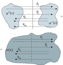
Figure 3: Optical theorem. Summation over $m$ and $n$ is assumed. The contributions of r.h.s. diagram are counted by the coordinates $(\gamma)$ of factor space $W$.

So, we restrict ourself by the direct calculation of the observable quantity, $\rho_{mn}$. This is crucial since allows to take into account the consequences of non-measurability of the quantum phase of amplitude $a_{mn}$ which is canceled in $\rho_{mn}$. Practically it is the additional for quantum systems dynamical principle of time reversibility, see the comment to Fig.4 and GCPr . It means that all acting in the system forces must compensate each other strictly in the frame of condition (15) , i.e. in the quantum case we have new equation of motion instead of (1), see (14):

$$\frac{\delta S(\varphi)}{\delta\varphi({\mathbf{x}},t)}=-\hbar j({\mathbf{x}},t)$$ (16)

if interaction with external field is switched on adiabatically. In opposite case the $z$-dependent term appears in the r.h.s. of Eq. (16). The source (force) $j({\mathbf{x}},t)$ in Eq. (16) generates quantum excitations. We will search the solutions of Eq. (16) expanding them in vicinity $j=0$.

A short qualitative description of corresponding to (16) generalized corresponding principle (GCP) one can find in GCPr , the detailed derivation of Eq. (16) is given in the review paper prepr . Notice also that (16) is reduced to the correspondence principle of Bohr in the limit $\hbar=0$. GCP means that the contributions into functional integral for $\rho_{mn}$ are defined by the complete set of solutions of strict equation (16) prepr . This is why we can act ex adverso: Eq. (16) defines all necessary and sufficient real time contributions into $\rho_{mn}$.

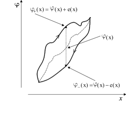
Figure 4: The dynamics along the mean trajectory $\varphi(x)$ is time reversible since the total action $S(\varphi_{+})-S^{*}(\varphi_{-})=S(\varphi_{+})+S(\varphi_{-})$ describes closed path motion, $<in|out><in|out>^{*}=<in|out><out|in>$, in the frame of boundary condition (15).

As the result, to find $R(z)$ in the frame of ordinary canonical scheme, see e.g. goldst ; jakiw ; fadde

(I) one must start from the equation:

$$\frac{\delta S(\varphi)}{\delta\varphi(x)}=0,$$ (17)

see the GCP representation (8). Having the solution $u(x)$ of this equation
(II) one can find $u_{j}(x;u)$ from the complete equation:

$$u_{j}:~{}\frac{\delta S(\varphi)}{\delta\varphi(x)}=j(x),~{}u_{j}(x)|_{j=0}=u(x),$$ (18)

in the form of the series over $j(x)$. It is evident that in that case we describe perturbations in the vicinity of $u(x)$. The same problem is solved in the stationary phase method. This step is reduced practically to the search of the particles propagator in the ”external field” $u(x)$. Generally this problem is unsolvable since in this case the 4-momentum is not conserved along particles trajectory. It must be noted that the expansion of $u_{j}$ over $j$ leads to the expansion over positive powers of interaction constant, i.e. presents the ”weak-coupling” expansion.

(III) Next,

$$\rho_{mn}=e^{-i\hat{\mathbb{K}}(j,e)}\sum_{\{u_{c}\}}e^{iU(u_{j},e)}{N(u_{j})}^{m}{N^{*}(u_{j})}^{n}\det(u_{j})^{-1},$$ (19)

where $\det(u_{j})$ is the functional determinant:

$$\det(u_{j})^{-1}=\int\prod_{x}d\varphi(x)\delta\left(\frac{\delta^{2}S(u_{j})}{\delta u_{j}(x)^{2}}\varphi(x)\right).$$

(IV) The last step is the calculation of the perturbation series generated by the operator $\hat{\mathbb{K}}$. Partial cancelation of contributions, which leads to the $\delta$-like measure (14), unchange the convergence radii. It can be shown that the obtained perturbation series has zero convergence radii prepr .

It is not hard to see that the naive use of solution of Eq. (18) leads to $\Gamma(q;u_{j})\neq 0$.

III Theories with symmetry

The crucial point of our analysis is the observation that $\Gamma(q;u)$ stocks up on the remote hypersurface $\sigma_{\infty}$ and that the external particle belongs to mass shell, $q^{2}=0$. Indeed, the vertex $\Gamma$ can be rewritten identically in the form:

$$\Gamma(q;\varphi)=\int dx\partial_{\mu}\left((\partial^{\mu}+2iq^{\mu})e^{-iqx}\varphi(x)\right)$$ (20)

if $q^{2}=0$ and $\varphi$ is the nonsingular function.

Our aim is to investigate $\Gamma(q;u)$, where $u(x)$ is the solution of Eq. (17), in all orders over $\hbar$ in the frame of the condition that the energy of $u(x)$ is finite:

$$H(u)=\int d{\mathbf{x}}\left(\frac{1}{2}(\partial_{t}u)^{2}+\frac{1}{2}(\nabla u)^{2}+v(u)\right)<\infty.$$ (21)

It will be shown that $\Gamma(q;u)=0$ since actually $u(x)$ is the nonsingular well localized object even in quantum case, i.e. (21) is rightful in all orders of $\hbar$.

The way of calculation of $\rho_{mn}$ shown at the end of previous Section is quite cumbersome. Moreover, the effect of ”symmetry breaking by $u({\mathbf{x}},t)$” is hidden in this approach, there is no obvious way to find the consequences of symmetry constraints. That is why the another way of computation of integral (8) was chosen.

Having a theory on $\delta$-like measure (14) one may adopt such most powerful method of classical mechanics as the transformation of variables, see also prepr . This is the one of important consequences of $\delta$-likeness of measure (14). We will consider in present paper the transformation,

$$u:~{}\varphi({\mathbf{x}},t)\rightarrow~{}\gamma(t)\in W,$$ (22)

where the new finite set of ”fields”, $\{\gamma\}$, are the functions only of the time, $t$, see also Fig.3. Noting that $\varphi({\mathbf{x}},t)$ is the function of $continuous~{}set$ of variable ${\mathbf{x}}$ and that the new ”fields” $\gamma_{i}(t)$ is labeled by the $countable~{}set$ of the indexes, $i=1,2,...,\nu,$ the mapping (22) means infinite reduction. This reduction of degrees of freedom is the main formal problem considered in details in present Section, see also prepr .

It must be noted also that the used formalism is Lorenz non-covariant. For this reason we will distinguish space and time components, $x=({\mathbf{x}},t)$. This circumstance is not crucial since we calculate the cross section, $\rho_{mn}$, which always is defined in the definite Lorenz frame. We will explain in the Appendix B why the general case $\gamma=\gamma({\mathbf{x}},t)$ have not been realized. So, we will not pay attention during subsequent calculations to the space components, ${\mathbf{x}}$, since they are the insufficient variables. Actually $u({\mathbf{x}},t)$ would be the singular distribution function of time because of the quantum perturbations tmf but we will see that the singularities of $u({\mathbf{x}},t)$ are integrable and do not gives an influence on the final result (2).

The transformation (22) is generated by a strict solution, $u({\mathbf{x}},t;\gamma_{0})$, of the Lagrange equation (1) where $\{\gamma_{0}\}$ is the set of integration constants. The complete set of solutions of nonlinear $4d$ equations of motion like (1) is unknown and we are forced to assume that the classical field, $u({\mathbf{x}},t;\gamma_{0})$, of necessary property (21) exists. This is a main lead-in assumption of the approach, the explicit form of $u({\mathbf{x}},t;\gamma_{0})$ will not be important for us.

The set of new fields, $\{\gamma(t)\}$, will be defined by the set $\{\gamma_{0}\}$, i.e. we will describe quantum dynamics mapping the problem with symmetry into the factor space $W$,

$$\{\gamma(t)\}_{t=0}=\{\gamma_{0}\}\in W.$$

The approach goes back to the old idea of statistical systems description in terms of collective variables bogol . The simple explanation of topology side of the transformation (22) was described in the transparent papers smalee , see also textbook arnoldd and marsden . The paper fadde is also useful since clarify Hamilton description to the extended, soliton, field configurations, farther details one can find in takhta . One can note also existence of the suggestion nohl to leave the frame of canonical schemes to quantize the extended fields.

Actually our approach to the quantum field theory with symmetry consists from two parts. First one stands of the mapping into $W=G/G_{w}$, where $G_{w}\in G$ is the symmetry group of $u$ . The second one contains dynamics, see also fadde . The problem of quantization comes into existence only in the second part.

One can call following useful geometrical interpretation of the ”collective variables” approach prepr . The set of parameters $\{\gamma_{0}\}$ form the factor space $W$ and $u({\mathbf{x}},t;\gamma_{0})$ belongs to it completely. The mapping of dynamics into $W$ form in it the finite-dimensional hypersurface. For example, the hypersurface compactify into the Arnold’s hypertorus if the classical system is completely integrable, see additional references in arnoldd and takhta . Then half of parameters $\gamma$ are the radii of the hypertorus and other half are the angles.

Description of quantum system in terms of the collective-like variables $\gamma(t)$ means the description of random deformations of such hypersurface, i.e. of the surface of Arnold’s hypertorus in the case of completely integrable system. That is why our approach describes just the fluctuations of $u({\mathbf{x}};\gamma(t))$ at the expense of fluctuations of $\gamma(t)$. Therefore, our formalism describes the fluctuations of $u(x)$, instead of usually considered canonical formalism which describes the fluctuations in the vicinity of $u(x)$, Sec.2.2.

Therefore, the main step of our calculations is the reduction of field-theoretical problem with symmetry to the quantum-mechanical one, where $(\xi(t),\eta(t))\in\{\gamma(t)\}$ are the generalized coordinates and momenta of the particle which is moving in $W$. It should be noted that in the frame of to-day knowledge it is impossible to present the complete set of first integrals of motion in involution considering the equations of type (1). Nevertheless we incline to interpret the reduction of degrees of freedom (22) as the consequence of symmetry constraints .

It is evident that being the infrared stable the quantum-mechanical perturbations of $\gamma(t)$ unchange the conclusion that $u(x)$ is the well localized field, i.e. $u(x)|_{x\in\sigma_{\infty}}=0,~{}\forall\hbar$. That is why we come to (2) in all orders over $\hbar$.

III.1 Mapping into $T^{*}W$

The method of transformation (22) looks as follows prepr . One can simplify calculations considering the case of $N(z;\varphi)=1$ since interactions with external fields are switched on adiabatically. Then we have:

$$\rho_{0}=\lim_{j=e=0}e^{-i\hat{\mathbb{K}}(j,e)}\int DMe^{iU(\varphi,e)},$$ (23)

where $U(\varphi,e)$ is the odd functional over $e$ and

$$2\hat{\mathbb{K}}(j,e)={\rm Re}\int_{C^{+}}d{\mathbf{x}}dt\frac{\partial}{\partial j({\mathbf{x}},t)}\frac{\partial}{\partial e({\mathbf{x}},t)},$$ (24)

$$DM=\prod_{{\mathbf{x}},t}d\varphi({\mathbf{x}},t)\delta(\partial_{\mu}^{2}\varphi({\mathbf{x}},t)+v^{\prime}(\varphi)-j({\mathbf{x}},t)).$$ (25)

One may shift Mills time contour $C^{+}$, see (9), on the real time axis since the description of fluctuations of $u({\mathbf{x}};\gamma)$ in terms of $\gamma(t)$ would be free from light-cone singularities prepr . This slightly simplifies calculations but the analytical continuation on the real time axis should be done carefully if $u(x)$ have nontrivial topology tmf , see also smalee .

The distinction of field theory from quantum mechanics consists in the presence of the space degrees of freedom. To look into this problem let us consider the formalism on the ”smoothed” $\delta$-function:

$$\lim_{\epsilon=0}\delta_{\epsilon}(x)=\delta(x).$$ (26)

It obeys the property of the ordinary $\delta$-function:

$$\int dxf(x)\delta_{\epsilon}(x-a)=f(a)(1+O(\epsilon)),~{}\epsilon\rightarrow 0.$$

At the same time $\delta_{\epsilon}(0)$ is finite,

$$\delta_{\epsilon}(0)=O(1/\epsilon).$$

Then, introducing the $auxiliary$ variable $\pi({\mathbf{x}},t)$:

$$1=\int\prod_{{\mathbf{x}},t}d\pi({\mathbf{x}},t)\delta(\pi({\mathbf{x}},t)-\dot{\varphi}({\mathbf{x}},t))$$ (27)

we come to the measure:

$$DM=\lim_{\epsilon=0}\prod_{{\mathbf{x}},t}d\varphi({\mathbf{x}},t)d\pi({\mathbf{x}},t)\delta_{\epsilon}\left(\dot{\varphi}({\mathbf{x}},t)-\frac{\delta H_{j}(\pi,\varphi)}{\delta\pi({\mathbf{x}},t)}\right)\delta_{\epsilon}\left(\dot{\pi}({\mathbf{x}},t)+\frac{\delta H_{j}(\pi,\varphi)}{\delta\varphi({\mathbf{x}},t)}\right).$$ (28)

The Hamiltonian looks as follows:

$$H_{j}=\int d{\mathbf{x}}\left\{\frac{1}{2}\pi^{2}({\mathbf{x}},t)+\frac{1}{2}(\nabla\varphi({\mathbf{x}},t))^{2}+v(\varphi)-j({\mathbf{x}},t)\varphi({\mathbf{x}},t)\right\}.$$ (29)

The independency of $\varphi$ and $\pi$ is not important for us. Introduction of the auxiliary variable $\pi$ is useful since in this case we come to the first order formalism and this will be important.

Let us introduce the unit:

$$1=\frac{1}{\Delta_{\epsilon}}\int\prod_{i=1}^{\nu}\prod_{t}d\xi_{i}(t)d\eta_{i}(t)\prod_{{\mathbf{x}},t}\delta_{\epsilon}(\varphi({\mathbf{x}},t)-u({\mathbf{x}};\xi,\eta))\delta_{\epsilon}(\pi({\mathbf{x}},t)-p({\mathbf{x}};\xi,\eta)),$$ (30)

where $u$ and $p$ are given functions of the $independent$ set of variables $\xi_{i}$ and $\eta_{i}$, $i=1,2,...,\nu$, and $\Delta_{\epsilon}$ is the normalization factor. We want to assume also that $\nu\geq 1$ and we expect that the equalities:

$$\varphi({\mathbf{x}},t)=u({\mathbf{x}};\xi(t),\eta(t)),~{}\pi({\mathbf{x}},t)=p({\mathbf{x}};\xi(t),\eta(t))$$ (31)

are satisfied under necessary for us choice of $\xi$ and $\eta$. The fact of the matter is that Eqs. (31) singles out definite parametrization of functions $\varphi({\mathbf{x}},t)$ and $\pi({\mathbf{x}},t)$. Therefore, we should think that substitution of $u$ and $p$ will transform the equalities:

$$\dot{\varphi}-\frac{\delta H_{j}(\pi,\varphi)}{\delta\pi}=0,~{}~{}\dot{\pi}+\frac{\delta H_{j}(\pi,\varphi)}{\delta\varphi}=0$$

into identities. This possibility is a consequence of the fact that both differential measures in (30) and (28) are $\delta$-like.

Let us introduce for sake of clearness the lattice in the ${\mathbf{x}}$ space with $n$ cells. Then (31) presents $n$ algebraic equalities for $\nu$ functions of time $(\xi_{i}(t),\eta_{i}(t)),~{}i=1,2,...,\nu$ which are independent from coordinate ${\mathbf{x}}$.

Next, let us assume that substitution of $(\bar{\xi}(t),\bar{\eta}(t))$ into Eqs. (31) transform them into the identities. Notice also that $\nu<n$. This means that the integral (30) is $\sim\delta_{\epsilon}^{(n-\nu)}(0)\sim(1/\epsilon)^{(n-\nu)}\rightarrow\infty$ at $\epsilon\rightarrow 0$. Therefore, considered transformation is singular.

Considering $(\bar{\xi}(t),\bar{\eta}(t))$ as the unique solution of (31) one can write that $\Delta_{\epsilon}=\Delta_{\epsilon}(\bar{\xi}(t),\bar{\eta}(t))$, where

$$\Delta_{\epsilon}(\bar{\xi},\bar{\eta})=\int\prod_{i=1}^{\nu}\prod_{t}d\tilde{\xi}_{i}d\tilde{\eta}_{i}\delta_{\epsilon}\left(\sum_{i=1}^{\nu}(u_{\bar{\xi}_{i}}\tilde{\xi}_{i}+u_{\bar{\eta}_{i}}\tilde{\eta}_{i})\right)\delta_{\epsilon}\left(\sum_{i=1}^{\nu}(p_{\bar{\xi}_{i}}\tilde{\xi}_{i}+p_{\bar{\eta}_{i}}\tilde{\eta}_{i})\right)$$ (32)

since $(\bar{\xi}_{i}(t),\bar{\eta}_{i}(t))$ are the necessary for us variables: the equalities

$$\sum_{i=1}^{\nu}(u_{\bar{\xi}_{i}}({\mathbf{x}};\bar{\xi},\bar{\eta})\tilde{\xi}_{i}+u_{\bar{\eta}_{i}}({\mathbf{x}};\bar{\xi},\bar{\eta})\tilde{\eta}_{i})=0,~{}~{}\sum_{i=1}^{\nu}(p_{\bar{\xi}_{i}}({\mathbf{x}};\bar{\xi},\bar{\eta})\tilde{\xi}_{i}+p_{\bar{\eta}_{i}}({\mathbf{x}};\bar{\xi},\bar{\eta})\tilde{\eta}_{i})=0$$ (33)

can be satisfied iff:

$$\tilde{\xi}_{i}(t)=0,~{}\tilde{\eta}_{i}(t)=0,i=1,2,...,\nu.$$ (34)

This solution is unique iff all $\bar{\xi}_{i}(t)$ and $\bar{\eta}_{i}(t)$ are independent even if $u$ and $p$ are not independent. Therefore, our only requirement is the absence of the additional, hidden, equalities of $f_{\alpha}(\bar{\xi},\bar{\eta})=0$ type, $\alpha=1,2...,$.

We perform the transformation (22) inserting the unite (30). As a result we come to the measure performing integration over $\varphi$ and $\pi$ firstly. Noting that the measures in (30) and in (28) are both $\delta$-like we find:

$$DM=\prod_{t}\prod_{i=1}^{\nu}\frac{d\xi_{i}(t)d\eta_{i}(t)}{\Delta(\bar{\xi},\bar{\eta})}\prod_{{\mathbf{x}},t}\delta_{\epsilon}\left(\dot{u}-\frac{\delta H_{j}(u,p)}{\delta p}\right)\delta_{\epsilon}\left(\dot{p}+\frac{\delta H_{j}(u,p)}{\delta u}\right)=$$

$$=\prod_{t}\prod_{i=1}^{\nu}\frac{d\xi_{i}(t)d\eta_{i}(t)}{\Delta(\bar{\xi},\bar{\eta})}\prod_{{\mathbf{x}},t}\delta_{\epsilon}\left(\sum_{i=1}^{\nu}u_{\xi_{i}}\dot{\xi}_{i}+\sum_{i=1}^{\nu}u_{\eta_{i}}\dot{\eta}_{i}-\frac{\delta H_{j}(u,p)}{\delta p}\right)\delta_{\epsilon}\left(\sum_{i=1}^{\nu}p_{\xi_{i}}\dot{\xi}_{i}+\sum_{i=1}^{\nu}p_{\eta_{i}}\dot{\eta}_{i}+\frac{\delta H_{j}(u,p)}{\delta u}\right).$$ (35)

Using the auxiliary integration method prepr one can diagonalize the arguments of last $\delta$-functions in (35). One can write:

$$DM=\prod_{t}\prod_{i=1}^{\nu}\frac{d\xi_{i}d\eta_{i}}{\Delta(\bar{\xi},\bar{\eta})}\int\prod_{t}\prod_{i=1}^{\nu}d\tilde{\xi_{i}}d\tilde{\eta_{i}}\delta\left(\tilde{\xi_{i}}-\left(\dot{\xi}_{i}-\frac{\partial h_{j}}{\partial\eta_{i}}\right)\right)\delta\left(\tilde{\eta_{i}}-\left(\dot{\eta}_{i}+\frac{\partial h_{j}}{\partial\xi_{i}}\right)\right)\times$$

$$\times\delta_{\epsilon}\left(\sum_{i=1}^{\nu}u_{\xi_{i}}\tilde{\xi}_{i}+\sum_{i=1}^{\nu}u_{\eta_{i}}\tilde{\eta}_{i}+\{u,h_{j}\}-\frac{\delta H_{j}(u,p)}{\delta p}\right)\delta_{\epsilon}\left(\sum_{i=1}^{\nu}p_{\xi_{i}}\tilde{\xi}_{i}+\sum_{i=1}^{\nu}p_{\eta_{i}}\tilde{\eta}_{i}+\{p,h_{j}\}+\frac{\delta H_{j}(u,p)}{\delta u}\right).$$ (36)

It is easy to see that (36) is identical to (35).

Let us assume now that $u({\mathbf{x}};\xi,\eta)$, $p({\mathbf{x}};\xi,\eta)$ and $h_{j}(\xi,\eta)$ are chosen so that

$$\{u,h_{j}\}=\frac{\delta H_{j}(u,p)}{\delta p},~{}~{}\{p,h_{j}\}=-\frac{\delta H_{j}(u,p)}{\delta u},$$ (37)

where Poisson bracket

$$\{u,h_{j}\}=\sum_{i=1}^{\nu}\left\{\frac{\partial u}{\partial\xi_{i}}\frac{\partial h_{j}}{\partial\eta_{i}}-\frac{\partial u}{\partial\eta_{i}}\frac{\partial h_{j}}{\partial\xi_{i}}\right\}$$

and the same we should have for $\{p,h_{j}\}$. Having in mind that the arguments of $\delta$-functions in (36) are accumulated near $\tilde{\xi}_{i}=\tilde{\eta}_{i}=0$ we come to the expression:

$$DM=\prod_{t}\prod_{i=1}^{\nu}\frac{d\xi_{i}d\eta_{i}}{\Delta_{\epsilon}(\bar{\xi},\bar{\eta})}\delta\left(\dot{\xi}_{i}-\frac{\partial h_{j}}{\partial\eta_{i}}\right)\delta\left(\dot{\eta}_{i}+\frac{\partial h_{j}}{\partial\xi_{i}}\right)\Delta_{\epsilon}(\xi,\eta),$$ (38)

where

$$\Delta_{\epsilon}(\xi,\eta)=\int\prod_{t}d\tilde{\xi}d\tilde{\eta}\prod_{{\mathbf{x}},t}\delta_{\epsilon}(u_{\xi}\tilde{\xi}+u_{\eta}\tilde{\eta})\delta_{\epsilon}(p_{\xi}\tilde{\xi}+p_{\eta}\tilde{\eta}).$$ (39)

have the same structure as (32).

The Jacobian of transformation is a ratio of determinants:

$$J=\Delta_{\epsilon}(\xi,\eta)/\Delta_{\epsilon}(\bar{\xi},\bar{\eta}),$$

where $(\bar{\xi},\bar{\eta})$ are the solutions of Eqs. (30) and $(\xi,\eta)$ are the solutions of equations

$$\dot{\xi}-\frac{\partial h_{j}}{\partial\eta}=0,~{}~{}\dot{\eta}+\frac{\partial h_{j}}{\partial\xi}=0,$$ (40)

as it follows from (38).

It is not too hard to understand that the set of variables $(\xi,\eta)$ in (39) is the same as in (32) since $u$ and $p$ must be chosen equal to the solutions of the incident equations. Indeed, taking into account (40) and then (37),

$$\dot{u}=\sum_{i=1}^{\nu}(u_{\xi_{i}}\dot{\xi}_{i}+u_{\eta_{i}}\dot{\eta}_{i})=\{u,h_{j}\}=\frac{\delta H_{j}}{\delta p},~{}~{}~{}~{}\dot{p}=\sum_{i=1}^{\nu}(p_{\xi_{i}}\dot{\xi}_{i}+p_{\eta_{i}}\dot{\eta}_{i})=\{p,h_{j}\}=-\frac{\delta H_{j}}{\delta u}.$$

As the result the Jacobian of the considered transformation is equal to one, $J=1$, since the arguments of (39) and (32) are equal to the one of the other.

The disappearance of $J$ leads to the absence of explicit dependence from ${\mathbf{x}}$. At the end one may choose $\epsilon=0$ and turn to the continuous ${\mathbf{x}}$ taking $n=\infty$. As a result:

$$DM=\prod_{t}\prod_{i=1}^{\nu}d\xi_{i}d\eta_{i}\delta\left(\dot{\xi}_{i}-\frac{\partial h_{j}}{\partial\eta_{i}}\right)\delta\left(\dot{\eta}_{i}+\frac{\partial h_{j}}{\partial\xi_{i}}\right).$$ (41)

The $ansatz$:

$$H_{j}(u,p)=h_{j}(\xi,\eta)$$ (42)

is natural since $u$ and $p$ must obey the incident equations. At the end, Eq. (37) defines the parametrization of $u$ and $p$ in terms of $\xi(t)$ and $\eta(t)$ and the dynamics is defined by functional $\delta$-functions in the measure (41), see Eqs. (40).

One can note definite conformity of considered transformation with canonical method of Hamilton mechanics in which the mechanical problem is divided into two parts, see e.g. arnoldd . In our case of the field theory with symmetry the problem also consists of two steps. First one is mapping of $\varphi({\mathbf{x}},t)$, and $\pi({\mathbf{x}},t)$, into factor space $W$, i.e. the first step is the definition of functional parametrization $u({\mathbf{x}};\xi,\eta)$ and $p({\mathbf{x}};\xi,\eta)$. One should assume at this point that we must solve Eqs. (37) together with (42) to find $u({\mathbf{x}};\xi,\eta)$ and $p({\mathbf{x}};\xi,\eta)$. The second step is the dynamical problem: one must solve Eqs. (40) expanding solutions over $j({\mathbf{x}},t)$. This may lead to contradiction with an assumption that $(\xi,\eta)$ are ${\mathbf{x}}$ independent quantities. The reason why the solution $(\xi({\mathbf{x}},t),~{}\eta({\mathbf{x}},t))$ is impossible is shown in Appendix B. It will be shown in the subsequent Subsection that the dependence of $j$ on ${\mathbf{x}}$ can not inspire the problems.

III.2 Mapping into $T^{*}W\times C$

We shall consider the mostly general factor space:

$$W=T^{*}W+C,$$ (43)

where $C$ is the zero modes manifold. Eq. (43) means that we wish to consider the system which is not completely integrable in the semiclassical limit: the conditions of Liouville-Arnold theorem arnoldd are not hold for it and $W$ can be compactified in that case only partly. Generally $W$ in the case (43) presents the hypertube. Its normal cross-section gives the compact manyfold with $(\xi,\eta)$ coordinates. Following to the general quantization rules only this canonical pare(s) must be quantized. It will be shown that the remaining variables, $\lambda$, are $c$-numbers, $\lambda\in C$ . The problem of extraction of $T^{*}W$ subspace from $W$ can not be solved without knowledge of explicit form of $u({\mathbf{x}},t;\gamma_{0})$ and we would assume that $T^{*}W$ is not the empty space .

The strictness of Eq. (16) in addition shows how $j({\mathbf{x}},t)$ must be transformed if $\varphi$ is transformed. Just this consequence allows to define the structure of $W$. Corresponding to (22) map of $j({\mathbf{x}},t)$ looks as follows: $j({\mathbf{x}},t)\rightarrow(j_{\xi}(t),j_{\eta}(t)),$ where $j_{\xi}$ and $j_{\eta}$ are the random forces acting along axes $\xi$ and $\eta$.

Following to (42),

$$h_{j}(\xi,\eta)=h(\xi,\eta)+\int d{\mathbf{x}}u({\mathbf{x}};\xi,\eta)j({\mathbf{x}},t).$$ (44)

Therefore

$$DM=\prod_{t}\prod_{i}d\xi_{i}(t)d\eta_{i}(t)\delta\left(\dot{\xi}_{i}(t)-\omega_{\eta_{i}}(\xi,\eta)-\int d{\mathbf{x}}\frac{\partial u({\mathbf{x}},\xi,\eta)}{\partial\eta_{i}(t)}j({\mathbf{x}},t)\right)\times$$

$$\times\delta\left(\dot{\eta}_{i}(t)+\omega_{\xi_{i}}(\xi,\eta)+\int d{\mathbf{x}}\frac{\partial u({\mathbf{x}},\xi,\eta)}{\partial\xi_{i}(t)}j({\mathbf{x}},t)\right),$$ (45)

where

$$\omega_{X_{i}}=\frac{\partial h}{\partial X_{i}},~{}X=(\xi,\eta),$$ (46)

is the ”speed” in the $W$ space.

One may simplify calculations using the equality prepr :

$$\delta\left(\dot{\xi}(t)-\omega_{\eta}-\int d{\mathbf{x}}\frac{\partial u({\mathbf{x}},\xi,\eta)}{\partial\eta(t)}j({\mathbf{x}},t)\right)=\lim_{j_{\xi}=e_{\xi}=0}e^{-(i/2)\int dt\frac{\delta}{\delta j_{\xi}(t)}\frac{\delta}{\delta e_{\xi}(t)}}\times$$

$$\times e^{2i\int dte_{\xi}(t)\int d{\mathbf{x}}\frac{\partial u({\mathbf{x}},\xi,\eta)}{\partial\eta(t)}j({\mathbf{x}},t)}\delta\left(\dot{\xi}_{i}(t)-\omega_{\eta}-j_{\xi_{i}}(t)\right).$$ (47)

This equality follows from Fourier transformation of $\delta$-function. The same transformation of argument of second $\delta$-function in (45) can be done.

Inserting (47) into the expression for $\rho_{mn}$ the action of operator (9) gives new perturbations generating operator

$$2\hat{\mathbf{k}}(j,e)=\int dt\left\{\frac{\delta}{\delta j_{\xi}}\cdot\frac{\delta}{\delta e_{\xi}}+\frac{\delta}{\delta j_{\eta}}\cdot\frac{\delta}{\delta e_{\eta}}\right\}$$ (48)

and new auxiliary field

$$e_{c}({\mathbf{x}},t)=\left\{e_{\eta}(t)\cdot\frac{\partial u({\mathbf{x}};\xi,\eta)}{\partial\xi(t)}-e_{\xi}(t)\cdot\frac{\partial u({\mathbf{x}};\xi,\eta)}{\partial\eta(t)}\right\}.$$ (49)

At the very end of calculations one must take all $j_{\xi},~{}j_{\eta}$ and $e_{\xi},~{}e_{\eta}$ equal to zero. The transformed measure looks as follows:

$$DM=\prod_{t}\prod_{i=1}^{\nu}d\xi_{i}d\eta_{i}\delta(\dot{\xi}_{i}(t)-\omega_{\eta}-j_{\xi_{i}}(t))\delta(\dot{\eta}_{i}(t)+\omega_{\xi}+j_{\eta_{i}}(t)),$$ (50)

where new forces, $j_{\xi}(t),j_{\eta}(t)$ are ${\mathbf{x}}$ independent. Eqs. (48), (49), (50) and

$$\rho(z)=\lim_{\{\xi,\eta;e_{\xi},e_{\eta}\}=0}e^{-i\hat{\mathbf{k}}(j,e)}\int DMe^{-iU(u,e_{c})}e^{-N(z;u)}$$ (51)

form the transformed theory in which each degree of freedom is excited by individual source, $j_{\xi_{i}}$ and $j_{\eta_{i}}$ and the ${\mathbf{x}}$ dependence have been integrated.

Introduction of $(j_{\xi}(t),j_{\eta}(t))$ ends the mapping of quantum theory into the linear space $W$. The latter means that $W$ is an isotropic and homogeneous smalee and as the result the perturbation theory in $W$ is extremely simple. That is why the problem of $\rho_{mn}$ in $W$ becomes calculable in all orders of $\hbar$ even in the case $u({\mathbf{x}},t)\neq$ const. It must be noted also that (51) presents the expansion over $\hbar^{2}$  prepr . This is readily seen from the estimation: $U/\hbar=O(\hbar^{2})$

It is quite possible that not all parameters $\{\gamma\}\in W$ are $q$-numbers. To define the structure of factor space $W$ one must extract from $\{\gamma\}$ the set of the canonically conjugated pares. We leave for them the same notations $\xi$ and $\eta$. This set will form simplectic subspace, $\{\xi,\eta\}\in T^{*}W$. Through $\lambda$ we will denote other coordinates, $\lambda\in C$. It is suitable to introduce the conjugate to $\lambda$ the auxiliary variables $\alpha$:

$$DM=\prod_{t}d^{\nu}\xi(t)d^{\nu}\eta\delta^{(\nu)}(\dot{\xi}(t)-\omega_{\eta}-j_{\xi}(t))\delta^{(\nu)}(\dot{\eta}(t)+\omega_{\xi}+j_{\eta_{i}}(t))\times$$

$$\times\prod d\lambda(t)d\alpha\delta(\dot{\lambda}(t)-\omega_{\alpha}-j_{\lambda}(t))\delta(\dot{\alpha}(t)+\omega_{\lambda}+j_{\alpha}(t))$$

and

$$2\hat{\mathbf{k}}(j,e)=\int dt\left\{\frac{\delta}{\delta j_{\xi}}\cdot\frac{\delta}{\delta e_{\xi}}+\frac{\delta}{\delta j_{\eta}}\cdot\frac{\delta}{\delta e_{\eta}}+\frac{\delta}{\delta j_{\lambda}}\cdot\frac{\delta}{\delta e_{\lambda}}+\frac{\delta}{\delta j_{\alpha}}\cdot\frac{\delta}{\delta e_{\alpha}}\right\},$$

$$e_{c}({\mathbf{x}},t)=\left\{e_{\eta}(t)\cdot\frac{\partial u}{\partial\xi(t)}-e_{\xi}(t)\cdot\frac{\partial u}{\partial\eta(t)}\right\}+\left\{e_{\alpha}\cdot\frac{\partial u}{\partial\lambda(t)}-e_{\lambda}\cdot\frac{\partial u}{\partial\alpha(t)}\right\}$$

to search the consequences of such enlargement assuming that $u$ does not depend on $\alpha$:

$$\frac{\partial u}{\partial\alpha}\approx 0.$$ (52)

We want to show that only the canonically conjugate pares quantize. Having (52) $e_{c}$ looks as follows:

$$e_{c}({\mathbf{x}},t)=\left\{e_{\eta}(t)\cdot\frac{\partial u}{\partial\xi(t)}-e_{\xi}(t)\cdot\frac{\partial u}{\partial\eta(t)}\right\}+e_{\alpha}\cdot\frac{\partial u}{\partial\lambda(t)}$$ (53)

and

$$DM=\prod_{t}d^{\nu}\xi(t)d^{\nu}\eta\delta^{(\nu)}(\dot{\xi}(t)-\omega_{\eta}-j_{\xi}(t))\delta^{(\nu)}(\dot{\eta}(t)+\omega_{\xi}+j_{\eta_{i}}(t))\times$$

$$\times\prod d\lambda(t)d\alpha(t)\delta(\dot{\lambda}(t)-j_{\lambda}(t))\delta(\dot{\alpha}(t)+\omega_{\lambda}+j_{\alpha}(t)),$$

where the conditions (52) were taken into account. Therefore, dependence on $e_{\lambda}$ disappears in $e_{c}$, i.e.

$$2\hat{\mathbf{k}}(j,e)=\int dt\left\{\frac{\delta}{\delta j_{\xi}}\cdot\frac{\delta}{\delta e_{\xi}}+\frac{\delta}{\delta j_{\eta}}\cdot\frac{\delta}{\delta e_{\eta}}+\frac{\delta}{\delta j_{\alpha}}\cdot\frac{\delta}{\delta e_{\alpha}}\right\}.$$ (54)

since all derivatives over $e_{\lambda}$ are equal to zero. Next, as it follows from (54), the derivatives over $j_{\lambda}$ also disappears in $\hat{\mathbf{k}}$. For this reason we can put $j_{\lambda}=0$:

$$DM=\prod_{t}d^{\nu}\xi(t)d^{\nu}\eta\delta^{(\nu)}(\dot{\xi}(t)-\omega_{\eta}-j_{\xi}(t))\delta^{(\nu)}(\dot{\eta}(t)+\omega_{\xi}+j_{\eta_{i}}(t))\times$$

$$\times\prod d\lambda(t)\delta(\dot{\lambda}(t))d\alpha(t)\delta(\dot{\alpha}(t)+\omega_{\lambda}+j_{\alpha}(t)),$$

Remembering (52) one may perform the shift: $\dot{\alpha}\rightarrow\dot{\alpha}-\omega_{\lambda}-j_{\alpha}$. As a result:

$$DM=d\lambda(0)\prod_{t}d^{\nu}\xi(t)d^{\nu}\eta\delta^{(\nu)}(\dot{\xi}(t)-\omega_{\eta}-j_{\xi}(t))\delta^{(\nu)}(\dot{\eta}(t)+\omega_{\xi}+j_{\eta_{i}}(t)),$$

where the integral over $\alpha$ was omitted and the definition:

$$\int\prod_{t}d\lambda(t)\delta(\dot{\lambda}(t))=\int d\lambda(0)$$

was used.

Therefore, the formalism naturally extracts the set of $q$-numbers and defines the measure of integrals over $c$-numbers.

Let us introduce the coordinates $\eta$ through the condition:

$$h=h(\eta).$$ (55)

Then equation of motion in $T^{*}W$ space looks as follows:

$$\dot{\xi}=\frac{\partial h_{j}}{\partial\eta}=\omega(\eta)+j_{\xi},~{}~{}\dot{\eta}=-\frac{\partial h_{j}}{\partial\xi}=j_{\eta},$$ (56)

i.e. $\xi$ can be considered as the generalized coordinate and $\eta$ is the conserved in the semiclassical approximation canonically conjugate generalized momentum, when $j_{\xi}=j_{\eta}=0$. The Eqs. (56) have following exact solutions:

$$\eta_{j}(t)=\eta_{0}+\int_{0}^{+\infty}dt^{\prime}g(t-t^{\prime})j_{\eta}(t^{\prime})\equiv\eta_{0}+\eta(t;j),$$

$$\xi_{j}(t)=\xi_{0}+\int_{0}^{+\infty}dt^{\prime}g(t-t^{\prime})(\omega(\eta_{0}+\eta)+j_{\xi}(t^{\prime}))\equiv\xi_{0}+\omega(t;\eta_{0}+\eta)+\xi(t;j),$$ (57)

where the boundary conditions:

$$\xi(0)=\xi_{0},~{}~{}\eta(0)=\eta_{0}$$ (58)

were applied. So

$$\lim_{j=0}\eta_{j}=\eta_{0},~{}~{}\lim_{j=0}\xi_{j}=\omega_{0}+\omega(\eta_{0})t.$$ (59)

The Green function $g(t-t^{\prime})$ has the extremely simple form prepr :

$$g(t-t^{\prime})=\Theta(t-t^{\prime}),~{}~{}\Theta(0)=1.$$ (60)

This explains why the mapping into $W$ space is useful. Notice that the singularity of $g(t-t^{\prime})$ is integrable.

IV Mass-shell particle production

The result of integration over $\xi(t)$ and $\eta(t)$ looks as follows:

$$\rho_{mn}(z)=\lim_{\xi=\eta=e_{\xi}=e_{\eta}=0}e^{-i\hat{\mathbf{k}}(je)}\int dMe^{iU(u,e_{c})}N(z;u)^{m}N^{*}(z;u)^{n},$$ (61)

where

$$dM=d\lambda d\xi_{0}d\eta_{0}.$$

We will consider the simplest case: $\dim T^{*}W=2$ and

$$2\hat{\mathbf{k}}=\int_{-\infty}^{+\infty}dt\left\{\frac{\delta}{\delta\xi(t)}\Theta(t-t^{\prime})\frac{\delta}{\delta e_{\xi}(t^{\prime})}\right.+\left.\frac{\delta}{\delta\eta(t)}\Theta(t-t^{\prime})\frac{\delta}{\delta e_{\eta}(t^{\prime})}\right\}dt^{\prime}.$$ (62)

The functional $U$ can be written in the general form:

$$U(u,e_{c})=\int d{\mathbf{x}}d\tau(e_{c}^{3}({\mathbf{x}},\tau)u({\mathbf{x}};\xi(\tau),\eta(\tau))+...),$$ (63)

where the dots signify higher orders over $e_{c}^{2r+1},~{}r=2,3,...$ The auxiliary variable $e_{c}$:

$$e_{c}({\mathbf{x}},t)=\left\{e_{\eta}(t)\cdot\frac{\partial u({\mathbf{x}};\xi,\eta)}{\partial\xi(t)}-e_{\xi}(t)\cdot\frac{\partial u({\mathbf{x}};\xi,\eta)}{\partial\eta(t)}\right\}$$

was defined in (49) and

$$u({\mathbf{x}};\xi,\eta)=u({\mathbf{x}};\xi_{0}+\omega(t;\eta_{0}+\eta)+\xi(t),\eta_{0}+\eta(t)).$$ (64)

Notice that the integration in (62) is performed along real time axis. This becomes possible if $u(x)$ is the regular function. Otherwise we must conserve definition of theory on the complex time plane until the very end of calculations.

By definition $U$ must be the odd function of $e_{c}$, see (63) and (13). This generates following lowest over $U$ term:

$$\sim\hat{\mathbf{k}}^{3}U(u,e_{c})N(z;u)^{m}N^{*}(z;u)^{n}$$ (65)

and the common term of our perturbation theory is:

$$\sim\hat{\mathbf{k}}^{3l}U(u,e_{c})^{l}N(z;u)^{m}N^{*}(z;u)^{n}=\hat{\mathbf{k}}^{3l}O(\Gamma^{2(n+m)})$$ (66)

since

$$N(z,u)=\int d\omega_{1}(z,q)\Gamma(q;u)\Gamma^{*}(q;u),$$

see (7), where

$$\Gamma(q;u)=\int dxe^{-ixq}\partial^{2}u(x)=\int dx\partial_{\mu}(\partial^{\mu}+2iq^{\mu})\left\{e^{-iqx}\varphi(x)\right\},$$ (67)

see (20).

Notice that

$$\lim_{\xi=\eta=0}\Gamma(q;u)=0$$ (68)

because of the condition (20). We will consider the fields:

$$\lim_{t\rightarrow\pm\infty}u({\mathbf{x}},t;\xi_{0},\eta_{0})=\lim_{t\rightarrow\pm\infty}\partial_{t}u({\mathbf{x}},t;\xi_{0},\eta_{0})=0,~{}~{}\forall(\xi_{0},\eta_{0}),$$ (69)

assuming that this condition is rightful in the infinitesimal neighborhoods of $\xi_{0}$ and $\eta_{0}$.

The variational derivative over $\xi(t^{\prime})$ gives:

$$\frac{\delta}{\delta\xi(t^{\prime})}\lim_{t\rightarrow\pm\infty}(\partial_{t}+2iq_{0})\left.\left\{e^{-iqx}u({\mathbf{x}};\xi(t),\eta(t))\right\}\right|_{\xi=\xi_{0},\eta=\eta_{0}}=$$

$$=\lim_{t\rightarrow\pm\infty}(\partial_{t}+2iq_{0})\left\{e^{-i(q_{0}t-\mathbf{q}{\mathbf{x}})}\frac{\partial}{\partial\xi_{0}}u({\mathbf{x}},t;\xi_{0},\eta_{0})\right\}\delta(t-t^{\prime})$$ (70)

since the derivative is calculated in the vicinity $\xi_{0}$. The same we will have for higher derivatives:

$$\prod_{i=1}^{k}\frac{\delta}{\delta\xi(t_{i}^{\prime})}\prod_{j=1}^{l}\frac{\delta}{\delta\xi(t_{j}^{\prime})}\lim_{t\rightarrow\pm\infty}(\partial_{t}+2iq_{0})\left\{e^{-iqx}u({\mathbf{x}};\xi(t),\eta(t))\right\}=$$

$$=\lim_{t\rightarrow\pm\infty}(\partial_{t}+2iq_{0})\left.\left\{e^{-i(q_{0}t-\mathbf{q}{\mathbf{x}})}\frac{\partial^{k}}{\partial\xi_{0}^{k}}\frac{\partial^{l}}{\partial\eta_{0}^{l}}u({\mathbf{x}},t;\xi_{0},\eta_{0})\right\}\right|_{\xi=\xi_{0},\eta=\eta_{0}}\prod_{i=1}^{k}\delta(t-t_{i}^{\prime})\prod_{j=1}^{l}\delta(t-t_{j}^{\prime}).$$ (71)

Integration over $t_{i}^{\prime}$ and $t_{j}^{\prime}$ reduces $\delta$-functions into $\theta$-functions and last ones may restrict the range of integration over time variables $\tau$ of the convergent integrals, see Eq. (63) and Appendix A. Therefore, the asymptotic over $t$ is defined only by derivatives of $u({\mathbf{x}},t;\xi_{0},\eta_{0})$ over $\xi_{0}$ and $\eta_{0}$.

It is shown in Appendix A that if (69) is rightful then the same must exist for all derivatives over $\xi_{0}$ and $\eta_{0}$. This ends the prove of Eq. (2).

V Concluding remarks

— It is important to have in mind that the transformation (22) is singular, i.e. the inverse to (22) transformation is impossible. The latter is significant for self-consistence of the approach: Eq. (2) means that the generated by $u({\mathbf{x}},t;\gamma_{0})$ constraints are so important that even a notion of plane waves is lost in the theory, or, in other words, Eq. (2) means that the fluctuations of $\gamma(t)$ compose a complete set of contributions and there is no need to take into account other ones.

— Our general result, Eq. (2), can be extended on gluon production considering Yang-Mills theory as the theory with symmetry. But Gribov ambiguity gribovv prevents proving of Eq. (2) for non-Abelian gauge theory canonical formalism if $u\neq 0$. It can be shown at the same time that GCP based formalism gives in each order over $\hbar$ the gauge invariant terms and for this reason there is no necessity to extract gauge degrees of freedom in it. The tentative consideration of that solution was given in jmp-grib and the complete description will be published later.

— Transformed perturbation theory presents the expansion over $\hbar^{2}$, i.e. it is not the WKB expansion, see Appendix A. A short discussion of the structure of new perturbation series is given in prepr .

A few remarks concerning unsolved problems at the end of the paper.

— There exists two ways to compute $\rho_{mn}$ having the non-trivial $u(x)$. First one was described at the end of Sec.2 and the GCP based formalism is given in Sec.3. One can think that both methods must lead to the same result (2) since the primary formula (8) is the same for both approaches. But I can not prove this equivalence because of extremal complexity of the first approach. It is possible that the problem is connected with transparent mechanism of accounting of the symmetry constraints in the canonical formalism. Notice that the mapping into the simplectic space $T^{*}W$ is the one of possible ways to realize Dirac’s diracc programm.

— It must be noted that if $u(x)$ have finite energy then GCP formulas are applicable at all distances and does not require infrared dimensional parameter $\Lambda$. It is not clear for this reason how to join GCP approach with canonical formalism.

— There exists the problem with interaction at small distances where the perturbative QCD formalism is presumably strict. For example, it is unclear how to explain the ”asymptotic freedom” effect in the GCP formalism since it is impossible to introduce the ”running coupling constant” in the GCP strong coupling perturbation theory over inverse interaction constant, see the example in Appendix A, without divergences and without even notion of ”gluon”.

— The enlargement of the GCP approach on the non-Abelian gauge theories assumes presence of the quark fields. This will be possible if the quark fields contribution is the invariant of the factor group $G/G_{w}$ prepr since only in this case the fields of quark sector do not give an influence on the vector fields.

— By all appearance, if the unitary $S$-matrix exists in the general relativity then even the notion of ”graviton” disappeared in this theory. In other words, the quantum perturbations must be described in terms of the fluctuations of metric, $u_{\mu\nu}$, under the conditione that $u_{\mu\nu}\in W$ since the general relativity symmetry constraints must be taken into account. The question of singular metric demands separate consideration.

I hope to look into some of this questions in the subsequent publications.

VI Appendix A. Example of massless $\varphi^{4}$ theory

Let us consider

$$\rho_{10}=\lim_{\xi=\eta=e_{\xi}=e_{\eta}=0}e^{-i\hat{\mathbf{k}}(je)}\int dMe^{iU(u,e_{c})}N(u),$$ (a.1)

where $N(u)=N(z;u)|_{z=1}$,

$$N(u)=\int\frac{d\mathbf{q}}{(2\pi)^{3}q_{0}}\Gamma(q;u)\Gamma^{*}(q;u),~{}q_{0}=+\sqrt{\mathbf{q}^{2}}$$ (a.2)

with

$$\Gamma(q;u)=\int d{\mathbf{x}}\int_{-\infty}^{+\infty}dt\partial_{t}\left[e^{-iqx}(\partial_{t}+iq)u({\mathbf{x}};\xi_{j},\eta_{j})\right]$$ (a.3)

equal to zero if $\xi_{j}(t)=\xi_{0}$ and $\eta_{j}(t)=\eta_{0}$, i.e.

$$\Gamma(q;u)|_{j=0}=0$$ (a.4)

The operator

$$2\hat{\mathbf{k}}(j,e)=\int_{-\infty}^{+\infty}dt\left\{\frac{\delta}{\delta j_{\xi}(t)}\frac{\delta}{\delta e_{\xi}(t)}+\frac{\delta}{\delta j_{\eta}(t)}\frac{\delta}{\delta e_{\eta}(t)}\right\}$$ (a.5)

and

$$e_{c}({\mathbf{x}},t;\xi_{j},\eta_{j})=\left\{e_{\eta}(t)\frac{\partial u({\mathbf{x}};\xi_{j}(t),\eta_{j}(t))}{\partial\xi_{0}}-e_{\xi}(t)\frac{\partial u({\mathbf{x}};\xi_{j}(t),\eta_{j}(t))}{\partial\eta_{0}}\right\}$$ (a.6)

To generate perturbation series one should expand the operator:

$$e^{-i\hat{\mathbf{k}}(je)}=\sum_{n_{\xi},n_{\eta}=0}^{\infty}\frac{(-i/2)^{n_{\xi}+n_{\eta}}}{n_{\xi}!n_{\eta}!}\int_{-\infty}^{+\infty}\prod_{l_{\xi}=1}^{n_{\xi}}dt_{l_{\xi}}\frac{\delta}{\delta j_{\xi}(t_{l_{\xi}})}\frac{\delta}{\delta e_{\xi}(t_{l_{\xi}})}\prod_{l_{\eta}=1}^{n_{\eta}}dt^{\prime}_{l_{\eta}}\frac{\delta}{\delta j_{\eta}(t^{\prime}_{l_{\eta}})}\frac{\delta}{\delta e_{\eta}(t^{\prime}_{l_{\eta}})}$$

Let us consider now the expansion:

$$e^{iU(u,e_{c})}=\sum_{n_{\xi},n_{\eta}=0}^{\infty}\int_{-\infty}^{+\infty}\prod_{k_{\xi}=1}^{n_{\xi}}dt_{k_{\xi}}e_{\xi}(t_{k_{\xi}})\prod_{k_{\eta}=1}^{n_{\eta}}dt^{\prime}_{k_{\eta}}e_{\xi}(t^{\prime}_{k_{\eta}})C_{n_{\xi},n_{\eta}}(u;t_{1},...,t_{n_{\xi}},t^{\prime}_{1},...,t^{\prime}_{n_{\eta}}),$$

where part of $C_{n_{\xi},n_{\eta}}$ may be equal to zero. Therefore,

$$\lim_{e_{\xi}=e_{\eta}=0}e^{-i\hat{\mathbf{k}}(je)}e^{iU(u,e_{c})}=\sum_{n_{\xi},n_{\eta}=0}^{\infty}\int_{-\infty}^{+\infty}\prod_{k_{\xi}=1}^{n_{\xi}}dt_{k_{\xi}}\frac{-i\delta}{2\delta j_{\xi}(t_{l_{\xi}})}\prod_{k_{\xi}=1}^{n_{\eta}}dt_{k_{\eta}}\frac{-i\delta}{2\delta j_{\eta}(t_{l_{\eta}})}\times$$

$$\times C_{n_{\xi},n_{\eta}}(u;t_{1},...,t_{n_{\xi}},t^{\prime}_{1},...,t^{\prime}_{n_{\eta}})=\hat{O}e^{iU(u,\hat{e}_{c})},$$

where

$$2i\hat{e}_{c}=\left\{\frac{\delta}{\delta j_{\eta}(t)}\frac{\partial u({\mathbf{x}};\xi_{j}(t),\eta_{j}(t))}{\partial\xi_{0}}-\frac{\delta}{\delta j_{\xi}(t)}\frac{\partial u({\mathbf{x}};\xi_{j}(t),\eta_{j}(t))}{\partial\eta_{0}}\right\}.$$ (a.7)

As the result, one can rewrite (a.1) in the form:

$$\rho_{10}=\lim_{\xi=\eta=0}\int dM\hat{O}e^{iU(u,\hat{e}_{c})}N(u),$$ (a.8)

where $\hat{O}$ means that the derivatives should stay to the left of all function on which it act. Considering the model (3) one can find $u\sim g^{-1/2}$, see Eq. (1), and

$$U(u,\hat{e}_{c})=g\int d{\mathbf{x}}dt\hat{e}_{c}^{3}u.$$ (a.9)

Therefore, expansion over $U(u,\hat{e}_{c})$ gives series over $1/g$. Taking into account (a.3) it is easy to see that the lowest order gives the term $\sim U(u,\hat{e}_{c})^{2}$. Next, one can find that $\hat{e}_{c}\sim\hbar$ in the units of $\hbar$. Therefore the expansion over $(U/\hbar)$ generates series over $\hbar^{2}$. Notice also that each order over $\hbar^{2}$ is real, see (a.8).

Noting that $N=O(\Gamma^{2})$ and taking into account comment to (a.2) one can find inserting (a.9) into (a.8) that the lowest nonequal to zero contribution looks as follows:

$$\rho_{10}=\lim_{j_{\xi}=j_{\eta}=0}\int dM\hat{O}U(u,\hat{e}_{c})N(u)+...=$$

$$=\lim_{j_{\xi}=j_{\eta}=0}\int dM\int d{\mathbf{x}}_{1}\int_{-\infty}^{+\infty}dt_{1}\hat{O}[\hat{e}_{c}^{3}({\mathbf{x}}_{1},t_{1};\xi_{j},\eta_{j})u({\mathbf{x}}_{1};\xi_{j},\eta_{j})_{t_{1}}]N(u)+...$$

Let as consider for the sake of simplicity action of the first term in (a.7). Then:

$$\rho^{(1)}_{10}=\lim_{j_{\xi}=j_{\eta}=0}\int dM\int\frac{d\mathbf{q}_{1}}{(2\pi)^{3}q_{10}}\int d{\mathbf{x}}_{1}\int_{-\infty}^{+\infty}dt_{1}\hat{O}\times$$

$$\times\left[\frac{\delta}{\delta j_{\eta}(t_{1})}\frac{\partial u({\mathbf{x}}_{1};\xi_{j},\eta_{j})_{t_{1}}}{\partial\xi_{0}}\right]^{3}u({\mathbf{x}}_{1};\xi_{j},\eta_{j})_{t_{1}}\times$$

$$\times\Gamma(q_{1};u)\Gamma^{*}(q_{1};u)+...,$$ (a.10)

where the differential operators act on all right standing functions of $u$.

Taking into account the definition of $\Gamma$’s in (a.3) we should be interested just in the results of action of differential operators $\delta/\delta j_{\eta}(t_{1})$:

$$\lim_{j=0}\frac{\delta}{\delta j_{\eta}(t_{1})}\Gamma(u)=\lim_{j=0}\int d{\mathbf{x}}\int_{-\infty}^{+\infty}dt^{\prime}\partial_{t^{\prime}}\left[e^{-iqx}(\partial_{t^{\prime}}+iq_{0})\frac{\delta}{\delta j_{\eta}(t_{k})}u({\mathbf{x}},t^{\prime};\xi_{j},\eta_{j})\right]=$$

$$=\lim_{j=0}\int d{\mathbf{x}}\int_{-\infty}^{+\infty}dt^{\prime}\partial_{t^{\prime}}\left[e^{-iqx}(\partial_{t^{\prime}}+iq_{0})\frac{\partial u({\mathbf{x}},t^{\prime};\xi_{0},\eta_{0})}{\partial\eta_{0}}\frac{\delta\eta_{j}(t^{\prime})}{\delta j_{\eta}(t_{1})}\right].$$

Noting that

$$\eta_{j}(t^{\prime})=\eta_{0}+\int_{0}^{+\infty}dt^{\prime\prime}g(t^{\prime}-t^{\prime\prime})j_{\eta}(t^{\prime\prime})$$

we will have:

$$\frac{\delta\eta_{j}(t^{\prime})}{\delta j_{\eta}(t_{1})}=\int_{-\infty}^{+\infty}dt^{\prime\prime}\Theta(t^{\prime\prime})g(t^{\prime}-t^{\prime\prime})\delta(t^{\prime\prime}-t_{1}))=\Theta(t_{1})g(t^{\prime}-t_{1})$$

Therefore,

$$\lim_{j=0}\frac{\delta\Gamma(u)}{\delta j_{\eta}(t_{1})}=\int d{\mathbf{x}}^{\prime}\int_{-\infty}^{+\infty}dt^{\prime}\partial_{t^{\prime}}\left[e^{-i(q_{0}t^{\prime}-\mathbf{q}{\mathbf{x}}^{\prime})}(\partial_{t^{\prime}}+iq_{0})\frac{\partial u({\mathbf{x}}^{\prime},t^{\prime};\xi^{\prime}_{0},\eta_{0})}{\partial\eta_{0}}\Theta(t_{1})\Theta(t^{\prime}-t_{1})\right]$$ (a.11)

since $g(t-t^{\prime})=\Theta(t-t^{\prime})$. Using this result one nontrivial term in $\rho_{10}$ looks as follows:

$$\rho^{(1)}_{10}=\lim_{j_{\xi}=j_{\eta}=0}\int dM\int\frac{d\mathbf{q}_{1}}{(2\pi)^{3}q_{10}}\int d{\mathbf{x}}_{1}\int_{-\infty}^{+\infty}dt_{1}\times$$

$$\times\frac{\delta\Gamma(q_{1};u)}{\delta j_{\eta}(t_{1})}\frac{\delta\Gamma^{*}(q_{1};u)}{\delta j_{\eta}(t_{1})}\frac{\delta}{\delta j_{\eta}(t_{1})}\left\{\left[\frac{\partial u({\mathbf{x}}_{1};\xi_{j},\eta_{j})_{t_{1}}}{\partial\xi_{0}}\right]^{3}u({\mathbf{x}}_{1};\xi_{j},\eta_{j})_{t_{1}}\right\}+...,$$ (a.12)

where the higher derivatives of $\Gamma$ also were not shown for the sake of simplicity.

As it follows from (a.11) the derivatives of $\Gamma$’s are proportional to $\Theta$-functions which restricts the range of integration over $t_{1}$ and $t_{2}$. One can rewrite (a.12) in the form:

$$\rho^{(1)}_{10}=\lim_{j_{\xi}=j_{\eta}=0}\int dM\int\frac{d\mathbf{q}_{1}}{(2\pi)^{3}q_{10}}\int\prod_{k}d{\mathbf{x}}^{\prime}_{k}\int_{-\infty}^{+\infty}\prod_{l}dt^{\prime}_{l}\times$$

$$\times\partial_{t_{1}^{\prime}}\partial_{t_{2}^{\prime}}\left\{\left[e^{-i(q_{0}t_{1}^{\prime}-\mathbf{q}{\mathbf{x}}_{1}^{\prime})}(\partial_{t_{1}^{\prime}}+iq_{0})\frac{\partial u({\mathbf{x}}_{1}^{\prime},t_{1}^{\prime};\xi^{\prime}_{0},\eta_{0})}{\partial\eta_{0}}\right]\right.\times$$

$$\times\left.\left[e^{-i(q_{0}t_{2}^{\prime}-\mathbf{q}{\mathbf{x}}_{2}^{\prime})}(\partial_{t_{2}^{\prime}}+iq_{0})\frac{\partial u({\mathbf{x}}_{2}^{\prime},t_{2}^{\prime};\xi^{\prime}_{0},\eta_{0})}{\partial\eta_{0}}\right]\right.\times$$

$$\times\left.\int_{-\infty}^{+\infty}dt_{1}\Theta(t_{1})\Theta(t^{\prime}_{1}-t_{1})\Theta(t^{\prime}_{2}-t_{1})\frac{\delta}{\delta j_{\eta}(t_{1})}\left(\left[\frac{\partial u({\mathbf{x}}_{1};\xi_{j},\eta_{j})_{t_{1}}}{\partial\xi_{0}}\right]^{3}u({\mathbf{x}}_{1};\xi_{j},\eta_{j})_{t_{1}}\right)\right\}+...$$

Only the typical term was shown here. Therefore, we should investigate

$$\lim_{t^{\prime}_{1},t^{\prime}_{2}\rightarrow\pm\infty}\frac{\partial u({\mathbf{x}}_{1}^{\prime},t_{1}^{\prime};\xi^{\prime}_{0},\eta_{0})}{\partial\eta_{0}}\frac{\partial u({\mathbf{x}}_{2}^{\prime},t_{2}^{\prime};\xi^{\prime}_{0},\eta_{0})}{\partial\eta_{0}}$$ (a.13)

times the function which is finite in this limits, i.e. if this limits are equal to zero then $\rho_{10}$ is also equal to zero.

It is easy to see that if (69) is rightful then

$$\lim_{t\rightarrow\pm\infty}\frac{\partial^{k}}{\partial\xi_{0}^{k}}\frac{\partial^{l}}{\partial\eta_{0}^{l}}u({\mathbf{x}},t;\xi_{0},\eta_{0})=0.$$ (a.14)

Indeed, one can consider the expansion:

$$u({\mathbf{x}},t;\xi_{0}+\varepsilon_{\xi},\eta_{0}+\varepsilon_{\eta})=\sum_{n_{\xi},n_{\eta}=0}^{\infty}\frac{\varepsilon_{\xi}^{n_{\xi}}\varepsilon_{\eta}^{n_{\eta}}}{n_{\xi}!n_{\eta}!}\frac{\partial^{n}_{\xi}}{\partial\xi_{0}}\frac{\partial^{n}_{\eta}}{\partial\eta_{0}}u({\mathbf{x}},t;\xi_{0},\eta_{0})$$

for infinitesimal $\varepsilon_{\xi},~{}\varepsilon_{\eta}$. Therefore, if (69) is rightful for all $(\xi_{0},\eta_{0})$ then (a.14) is also rightful since $\varepsilon_{\xi},~{}\varepsilon_{\eta}$ are arbitrary. This proves (2) in all orders over $\hbar^{2}$.

VII Appendix B. Space-time local transformation

Let us consider the case: $\xi=\xi({\mathbf{x}},t)$ and $\eta=\eta({\mathbf{x}},t)$. In this case one must insert the unit:

$$1=\frac{1}{\Delta}\int D\xi D\eta\prod_{{\mathbf{x}},t}\delta(\varphi({\mathbf{x}},t)-u({\mathbf{x}},\xi({\mathbf{x}},t),\eta({\mathbf{x}},t)))\delta(\pi({\mathbf{x}},t)-p({\mathbf{x}},\xi({\mathbf{x}},t),\eta({\mathbf{x}},t))),$$ (b.1)

where $\Delta$ is the normalization factor,

$$D\xi D\eta=\prod_{{\mathbf{x}},t}\prod_{i}^{\nu}d\xi_{i}({\mathbf{x}},t)d\eta_{i}({\mathbf{x}},t)$$ (b.2)

and $(u,p)$ are given functions of ${\mathbf{x}}$ and $(\xi({\mathbf{x}},t),\eta({\mathbf{x}},t))$. The ”Hamiltonian” has the same form.

If the solution of equations:

$$\varphi({\mathbf{x}},t)=u({\mathbf{x}};\xi({\mathbf{x}},t),\eta({\mathbf{x}},t)),~{}~{}\pi({\mathbf{x}},t)=p({\mathbf{x}};\xi({\mathbf{x}},t),\eta({\mathbf{x}},t))$$ (b.3)

is $\bar{\xi}({\mathbf{x}},t),\bar{\eta}({\mathbf{x}},t)$ then, see (32):

$$\Delta(\bar{\xi},\bar{\eta})=\int D\tilde{\xi}D\tilde{\eta}\prod_{{\mathbf{x}},t}\delta\left(\sum_{i}^{\nu}\left\{u_{\bar{\xi}_{i}}({\mathbf{x}};\bar{\xi},\bar{\eta})\tilde{\xi}_{i}({\mathbf{x}},t)+u_{\bar{\eta}_{i}}({\mathbf{x}};\bar{\xi},\bar{\eta})\tilde{\eta}_{i}({\mathbf{x}},t)\right\}\right)\times$$

$$\times\delta\left(\sum_{i}^{\nu}\left\{\pi_{\bar{\xi}_{i}}({\mathbf{x}};\bar{\xi},\bar{\eta})\tilde{\xi}_{i}({\mathbf{x}},t)+\pi_{\bar{\eta}_{i}}({\mathbf{x}};\bar{\xi},\bar{\eta})\tilde{\eta}_{i}({\mathbf{x}},t)\right\}\right).$$ (b.4)

We should have again

$$\Delta^{-1}(\bar{\xi},\bar{\eta})\neq 0.$$ (b.5)

Using the method of auxiliary integration one come to the expression:

$$DM=\prod_{{\mathbf{x}},t}\prod_{i}^{\nu}d\xi_{i}d\eta_{i}\delta\left(\dot{\xi}_{i}-\frac{\delta h_{j}}{\delta\eta_{k}}\right)\delta\left(\dot{\eta}_{i}+\frac{\delta h_{j}}{\delta\xi_{k}}\right)\times$$

$$\times\frac{1}{\Delta(\bar{\xi},\bar{\eta})}\int D\tilde{\xi}D\tilde{\eta}\prod_{{\mathbf{x}},t}\delta\left(\sum_{i}^{\nu}\left\{u_{\xi_{i}}({\mathbf{x}};\xi,\eta)\tilde{\xi}_{i}(t)+u_{\eta_{i}}({\mathbf{x}};\xi,\eta)\tilde{\eta}_{i}(t)\right\}\right)\times$$

$$\times\delta\left(\sum_{i}^{\nu}\left\{\pi_{\xi_{i}}({\mathbf{x}};\xi,\eta)\tilde{\xi}_{i}(t)+\pi_{\eta_{i}}({\mathbf{x}};\xi,\eta)\tilde{\eta}_{i}(t)\right\}\right),$$ (b.6)

if the equations:

$$u_{\bar{\xi}_{i}}({\mathbf{x}};\bar{\xi},\bar{\eta})\tilde{\xi}_{i}({\mathbf{x}},t)=-u_{\bar{\eta}_{i}}({\mathbf{x}};\bar{\xi},\bar{\eta})\tilde{\eta}_{i}({\mathbf{x}},t),~{}\pi_{\bar{\xi}_{i}}({\mathbf{x}};\bar{\xi},\bar{\eta})\tilde{\xi}_{i}({\mathbf{x}},t)=-\pi_{\bar{\eta}_{i}}({\mathbf{x}};\bar{\xi},\bar{\eta})\tilde{\eta}_{i}({\mathbf{x}},t)$$

have the unique solution

$$\tilde{\xi}_{i}({\mathbf{x}},t)=\tilde{\eta}_{i}({\mathbf{x}},t)=0.$$

Let us assume that this conditions are satisfied. The ratio of determinants is again canceled for the same reasons as in (38)

At the same time we must have:

$$\{u({\mathbf{x}},\xi,\eta),h_{j}\}-\frac{\delta H_{j}}{\delta p({\mathbf{x}},\xi,\eta)}=0,~{}~{}\{p({\mathbf{x}},\xi,\eta),h_{j}\}+\frac{\delta H_{j}}{\delta u({\mathbf{x}},\xi,\eta)}=0,$$ (b.7)

where the Poisson bracket:

$$\{u({\mathbf{x}},\lambda),h_{j}\}=\frac{\partial u({\mathbf{x}},\xi({\mathbf{x}},t,),\eta({\mathbf{x}},t))}{\partial\xi({\mathbf{x}},t,)}\frac{\delta h_{j}}{\delta\eta({\mathbf{x}},t)}-\frac{\partial u({\mathbf{x}},\xi({\mathbf{x}},t,),\eta({\mathbf{x}},t))}{\partial\eta({\mathbf{x}},t,)}\frac{\delta h_{j}}{\delta\xi({\mathbf{x}},t)}$$

and the same for bracket $\{p({\mathbf{x}},\lambda),h_{j}\}$. Next, the Eqs. (b.7) together with the same equality for $\{p({\mathbf{x}},\lambda),h_{j}\}$ lead to the equal space-time Poisson equations:

$$\{u({\mathbf{x}},\xi({\mathbf{x}},t),\eta({\mathbf{x}},t)),u({\mathbf{x}},\xi({\mathbf{x}},t),\eta({\mathbf{x}},t))\}=\{p({\mathbf{x}},\xi,\eta),p({\mathbf{x}},\xi,\eta)\}=0$$ (b.8)

and

$$\{u({\mathbf{x}};\xi({\mathbf{x}},t),\eta({\mathbf{x}},t)),p({\mathbf{x}};\xi({\mathbf{x}},t),\eta({\mathbf{x}},t))\}=1$$ (b.9)

if the $ansatz$ (42) is taken into account. The last equality can not be satisfied since $u({\mathbf{x}},\xi,\eta)$ and $p({\mathbf{x}},\xi,\eta)$ are not the independent quantities.

Notes

1. a) The important question of symmetry constraints was considered in diracc .
2. b) This reminds the principle of d’Alembert.
3. c) The list of known solutions of Eq. (1) is given e.g. in actorr .
4. d) For example, $\gamma_{0}$ may define the space-time position of $u$-th maximum, its scale, etc. In other words the set $\{\gamma_{0}\}$ defines the integral, i.e. the ”collective”, form of $u({\mathbf{x}},t)$. Allowing for the symmetry constraints only the collective variables remain free takhta .
5. e) This explains why the definition: ”field theory with symmetry” was introduced. For example, $W=O(4,2)/O(4)\times O(2)$ in the conformal field theory with symmetry if $u$ is the $O(4)\times O(2)$-invariant solution of Eq. (1) dealf .
6. f) One can find the example of analogous reduction in the simplest completely integrable system in prepr . Our interpretation of the reduction is rightful in that case, see also takhta .
7. g) The example from quantum mechanics: $(angular~{}momentum,angle)\in T^{*}W$ are the $q$-numbers but $(length~{}of~{}Runge-Lenz~{}vector)\in C$ is the $c$-number in the $H$-atom problem prepr .
8. h) QED presents the example of empty $T^{*}W$.
9. i) Since the gauge invariant quantity, $\rho_{mn}$, is calculated

- (1) J.Goldstone and R.Jackiw, Phys. Rev., 11 (1975) 1486
- (2) R.Jackiw, Rev. Mod. Phys., 49 (1977) 681
- (3) J.Manjavidze, Phys. Part. Nucl., 43 (2012) 523, JINR Preprint, E2-2010-130, arXiv:1101.1193v2
- (4) J.Manjavidze and A.Sissakian, Theor. Math. Phys., 130 (2002) 153
- (5) P.Carruthers and F.Zachariasen, Rev.Mod.Phys., 55 (1983) 245; Phys.Rev., D13 (1986) 950
- (6) J.Manjavidze and A.Sissakian, Phys.Rep., 346 (2001) 1
- (7) J. Manjavidze, arXiv:1106.6181v1
- (8) L.D.Faddeev and V.E.Korepin, Phys. Rep., 42 (1978) 1
- (9) N.N.Bogolyubov and Tyablikov, JETP, 19 (1949) 256
- (10) S.Smale, Inv.Math., 10:4, 305 (1970), ibid., 11:1, 45 (1970)
- (11) V.I.Arnold Mathematical Methods of Classical Mechanics,(Springer, 1978)
- (12) R.Abraham and J.E.Marsden, Foundations of Mechanics (Benjamin/ Cummings Publ. Comp., Reading, Mass., 1978)
- (13) L.A.Takhtajan and L.D.Faddeev, Hamilton Methods in the Theory of Solitons (Springer, 2007)
- (14) R.Jackiw, C.Nohl and C.Rebbi, Preprint BNL-23772 (1977)
- (15) V.N.Gribov, Nucl. Phys., B139, 246 (1978); I.M.Singer, Comm. Math. Phys., 60 (1978) 7; M.F.Atiyah and J. D. S. Jones, Comm. Math. Phys., 61 (1978) 97
- (16) J.Manjavidze and A.Sissakian, J. Math. Phys., 42 (2001) 4158
- (17) P.A.M. Dirac, Lectures on Quantum Mechanics (Yeshiva Univ., New York, 1964)
- (18) A.Actor, Rev. Mod. Phys., 51 (1979) 461
- (19) V.De Alfaro, S.Fubini and G.Furlan, Phys. Lett., 65B (1976) 163; V.De Alfaro, S.Fubini and G.Furlan, Acta Phys. Austr. Suppl., XXII (1980) 51