Simplifying inclusion - exclusion formulas

Abstract.

Let $\mathcal{F}=\{F_{1},F_{2},\ldots,F_{n}\}$ be a family of $n$ sets on a ground set $S$, such as a family of balls in $\mathbb{R}^{d}$. For every finite measure $\mu$ on $S$, such that the sets of $\mathcal{F}$ are measurable, the classical inclusion-exclusion formula asserts that $\mu(F_{1}\cup F_{2}\cup\cdots\cup F_{n})=\sum_{I:\emptyset\neq I\subseteq[n]}(-1)^{|I|+1}\mu\Bigl{(}\bigcap_{i\in I}F_{i}\Bigr{)}$; that is, the measure of the union is expressed using measures of various intersections. The number of terms in this formula is exponential in $n$, and a significant amount of research, originating in applied areas, has been devoted to constructing simpler formulas for particular families $\mathcal{F}$. We provide an upper bound valid for an arbitrary $\mathcal{F}$: we show that every system $\mathcal{F}$ of $n$ sets with $m$ nonempty fields in the Venn diagram admits an inclusion-exclusion formula with $m^{O(\log^{2}n)}$ terms and with $\pm 1$ coefficients, and that such a formula can be computed in $m^{O(\log^{2}n)}$ expected time. For every $\varepsilon>0$ we also construct systems with Venn diagram of size $m$ for which every valid inclusion-exclusion formula has the sum of absolute values of the coefficients at least $\Omega(m^{2-\varepsilon})$.

1 Introduction

One of the basic topics in introductory courses of discrete mathematics is the inclusion-exclusion principle (also called the sieve formula), which allows one to compute the number of elements of a union $F_{1}\cup F_{2}\cup\cdots\cup F_{n}$ of $n$ sets from the knowledge of the sizes of all intersections of the $F_{i}$’s.

We will consider a slightly more general setting, where we have a ground set $S$ and a (finite) measure $\mu$ on $S$; then the inclusion-exclusion principle asserts that for every collection $F_{1},F_{2},\ldots,F_{n}$ of $\mu$-measurable sets, we have

$$\mu\biggl{(}\bigcup_{i=1}^{n}F_{i}\biggr{)}=\sum_{I:\emptyset\neq I\subseteq[n]}(-1)^{|I|+1}\mu\biggl{(}\bigcap_{i\in I}F_{i}\biggr{)}.$$ (1)

(Here, as usual, $[n]=\{1,2,\ldots,n\}$ and $|I|$ denotes the cardinality of the set $I$.) This principle not only plays a fundamental role in various areas of mathematics such as probability theory or combinatorics, but it also has important algorithmic applications. For instance, it provides simple methods for the computation of volume or surface area of molecules in computational biology [PCG⁺92] and underlies, through efficient computation of Möbius transforms [Knu97, Section 4.3.4], the best known algorithms for several NP-hard problems including graph $k$-coloring [BHK09], travelling salesman problem on bounded-degree graphs [BHKK08], dominating set [vRNvD09], or partial dominating set and set splitting [NvR10].

The inclusion-exclusion principle involves a number of summands that is exponential in $n$, the number of sets. In general this cannot be avoided if one wants an exact formula valid for every family $\mathcal{F}=\{F_{1},F_{2},\ldots,F_{n}\}$; see Example 2.3 below for a family for which Equation (1) is the only solution. Yet, since this is a serious obstacle to efficient uses of inclusion-exclusion, much effort has been devoted to finding “smaller” formulas. These efforts essentially organize along two lines of research.

The first approach gives up on exactness and tries to approximate efficiently the measure of the union using the measure of only some of the intersections. The first results of this flavor are the classical Bonferroni inequalities [Bon36]. It turns out that better approximations can be obtained by replacing the coefficients $(-1)^{|I|+1}$ by other suitable numbers, and such Bonferroni-type inequalities have been studied extensively; see, e.g., [Gal96]. Linial and Nisan [LN90] and Kahn et al. [KLS96] investigated how well $\mu(F_{1}\cup\cdots\cup F_{n})$ can be approximated if we know the measure of all intersections $\bigcap_{i\in I}F_{i}$ for all $I\subseteq[n]$ of size at most $r$. Their main finding is that having $r$ at least of order $\sqrt{n}$ is both necessary and sufficient for a reasonable approximation in the worst case. This still leaves us with about $2^{\sqrt{n}}$ terms in approximate inclusion-exclusion formulas.

The second line of research looks for “small” inclusion-exclusion formulas valid for specific families of sets. To illustrate the type of simplifications afforded by fixing the sets, consider the family $\mathcal{F}=\{F_{1},F_{2},F_{3}\}$ of Figure 1. Since $F_{1}\cap F_{3}=F_{1}\cap F_{2}\cap F_{3}$, Formula (1) can be simplified to

$$\mu\left(F_{1}\cup F_{2}\cup F_{3}\right)=\mu(F_{1})+\mu(F_{2})+\mu(F_{3})-\mu(F_{1}\cap F_{2})-\mu(F_{2}\cap F_{3}).$$

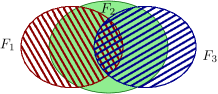
Figure 1: Three subsets of $\mathbb{R}^{2}$ admitting a simpler inclusion-exclusion formula. The ground set $F_{1}\cup F_{2}\cup F_{3}$ splits into six nonempty regions recognizable by the filling pattern.

More generally, let us consider a family $\mathcal{F}=\{F_{1},F_{2},\ldots,F_{n}\}$, and let us say that a coefficient vector

$$\boldsymbol{\alpha}=(\alpha_{I})_{\emptyset\neq I\subseteq[n]}\in\mathbb{R}^{2^{n}-1}$$

is an IE-vector for $\mathcal{F}$ if we have

$$\mu\biggl{(}\bigcup_{i=1}^{n}F_{i}\biggr{)}=\sum_{I\colon\emptyset\neq I\subseteq[n]}\alpha_{I}\mu\biggl{(}\bigcap_{i\in I}F_{i}\biggr{)}$$ (2)

for every finite measure $\mu$ on the ground set of $\mathcal{F}$ (with all the $F_{i}$’s measurable). Given $\mathcal{F}$, we would like to find an IE-vector for $\mathcal{F}$, such that both the number of nonzero coefficients is small, and the coefficients themselves are not too large. This idea, which we originally learned from [AE07], seems to originate in the work of Kratky [Kra78] on families of disks in the plane, and a systematic study of such simplifications was initiated by Naiman and Wynn [NW92, NW97]. A simplified inclusion-exclusion formula was also successfully used in an algorithm of Björklund et al. [BHKK08]. We refer to the monograph of Dohmen [Doh03] for an overview of this line of research.

Given a specific family $\mathcal{F}=\{F_{1},F_{2},\ldots,F_{n}\}$ of sets, how small can we expect an inclusion-exclusion formula to be? This is, roughly speaking, the question we tackle in this paper. To formalize the problem, we should specify how $\mathcal{F}$ is given. Let us consider the Venn diagram of $\mathcal{F}$, which is the partition of the ground set $S$ into equivalence classes according to the membership in the sets of $\mathcal{F}$. For each nonempty index set $\tau\subseteq[n]$, we define the region of $\tau$, denoted by $\textrm{reg}(\tau)$, as the set of all points that belong to the sets $F_{i}$ with $i\in\tau$ and no others (see Figure 1);

$$\textrm{reg}(\tau)=\biggl{(}\,\bigcap_{i\in\tau}F_{i}\,\biggr{)}\setminus\biggl{(}\,\bigcup_{i\not\in\tau}F_{i}\,\biggr{)}.$$

The Venn diagram of $\mathcal{F}$ is then the collection of all subsets of $[n]$ with non-empty regions; that is,

$$\mathcal{V}=\mathcal{V}(\mathcal{F}):=\{\tau\subseteq[n]\colon\textrm{reg}(\tau)\neq\emptyset\}.$$

We regard the Venn diagram as a set system on the ground set $[n]$; it is a “dual” of the set system $\mathcal{F}$.

We say that $\mathcal{F}$ is standardized if the ground set equals the union of the $F_{i}$’s and each nonempty region has exactly one point. It is easy to see that, as far as inclusion-exclusion formulas are concerned, all points in a single region are equivalent; it only matters which of the regions are nonempty. Therefore assuming that $\mathcal{F}$ is standardized does not mean a loss of generality. We will use this assumption in the algorithmic part of our main result—Theorem 1.1. For general $\mathcal{F}$ this requires a preprocessing step for $\mathcal{F}$, in which the part of the ground set $S$ in each nonempty region is contracted to a single point.

Let $\mathcal{F}=\{F_{1},F_{2},\ldots,F_{n}\}$ be a family of sets and let $m$ denote the size of $\mathcal{V}$ (which equals the size of the ground set for $\mathcal{F}$ standardized). A linear-algebraic argument shows that every (finite) family $\mathcal{F}$ has an inclusion-exclusion formula with at most $m$ terms (see Corollary 2.4) and $m$ terms are sometimes necessary (see the beginning of Section 4). The question of how small a formula $\mathcal{F}$ admits may thus seem settled. There is, however, a caveat: this linear-algebraic argument may yield exponentially large coefficients (see Example 2.6). If we wanted to use such a formula, we would need to compute with very high precision, and perhaps more seriously, we would have to know the measures of the various intersections with an enormous precision, in order to obtain a meaningful result. This may be totally impractical, e.g., in geometric settings where some physical measurements are involved, or where the measures of the intersections are computed with limited precision.Thus, we prefer inclusion-exclusion formulas where not only the number of terms is small, but the coefficients are also small.

Our main result is the following general upper bound; to our knowledge, it is the first upper bound applicable for an arbitrary family.

Theorem 1.1.

Let $n$ and $m$ be integers and let $D=\lceil 2e\ln m\rceil\lceil 2+\ln\frac{n}{\ln m}\rceil$. Then for every family $\mathcal{F}$ of $n$ sets with Venn diagram of size $m$, there is an IE-vector $\boldsymbol{\alpha}$ for $\mathcal{F}$ that has at most $\sum_{i=1}^{D}{\binom{n}{i}}\leq m^{O(\ln^{2}n)}$ nonzero coefficients, and in which all nonzero coefficients are $\pm 1$’s. Such an $\boldsymbol{\alpha}$ can be computed in $m^{O(\ln^{2}n)}$ expected time if $\mathcal{F}$ is standardized.

The bound in this theorem is quasi-polynomial, but not polynomial, in $m$ and $n$. We do not know if a polynomial bound can be achieved with $\pm 1$ coefficients. We have at least the following lower bound, proved in Section 4, showing that inclusion-exclusion formulas of linear size are impossible in general.

Theorem 1.2.

For any $\varepsilon>0$, for arbitrarily large values of $m$, there exists a family of sets with Venn diagram of size $m$ for which any IE-vector has $\ell_{1}$-norm at least $\Omega\left(m^{2-\varepsilon}\right)$.

We recall that the $\ell_{1}$-norm of a real vector $\boldsymbol{x}\in\mathbb{R}^{d}$ is $\|\boldsymbol{x}\|_{1}=\sum_{i=1}^{d}|x_{i}|$. The $\ell_{1}$-norm gives a lower bound on the tradeoff between the number of nonzero coefficients and their orders of magnitude (we recall that a formula with $O(m)$ nonzero coefficients is always attainable, the problem being that the coefficients may be too large).

Remark on $\ell_{1}$-norm minimization.

A useful heuristic for finding “small” IE-vectors might be to look for an IE-vector of minimum $\ell_{1}$-norm. In the linear-algebraic formulation, this means finding a solution of $A\boldsymbol{x}=\mathbf{1}$ of minimum $\ell_{1}$-norm.

It is well known that finding a solution of minimum $\ell_{1}$-norm of a linear system can be done in polynomial time, via linear programming. Several specialized algorithms for this problem have also been developed, with better performance than direct application of general-purpose LP solvers (see, e.g., [YGZ⁺10] for a recent overview). However, in our setting the number of columns of the matrix $A$ may be exponential in $m$ and $n$, and so even the input for an $\ell_{1}$-norm minimizing algorithm would be too large.

There are linear programs with exponentially many variables (and polynomially many constraints) that can still be solved in polynomial time. For example, one may attempt, at least for theoretical purposes, to solve the dual linear program by the ellipsoid method, provided that a separation oracle is available.

In our setting, the task of the separation oracle can be formulated as follows in the setting of the original (standardized) set system $\mathcal{F}=\{F_{1},\ldots,F_{n}\}$: Given weights $w_{1},\ldots,w_{m}\in\mathbb{Z}$ of the points and threshold $c$, find a subset $I\subseteq[n]$, if one exists, such that the sum of weights of the points in $\bigcap_{i\in I}F_{i}$ is at least $c$. Unfortunately, as was shown by Hoffmann et al. [HOR⁺12], this problem is NP-complete not only for arbitrary set systems, but also, e.g., for the case where each $F_{i}$ is the complement of a hexagon in the plane. Thus, this approach doesn’t seem to lead to a polynomial-time algorithm for finding an IE-vector of minimum $\ell_{1}$-norm even for rather simple geometric settings.

Topological background.

In order to prove Theorem 1.1 we need several basic notions from topological combinatorics. We aim at a self-contained exposition that should make the proof accessible even to a reader who is not familiar with topological methods (we use the topological background mostly indirectly). For further reading we refer the reader to sources such as [Hat01, Mat03, Mun84].

2 Preliminaries

We consider a family $\mathcal{F}=\{F_{1},F_{2},\ldots,F_{n}\}$ of sets on a ground set $S$, and assume that the $F_{i}$ are all distinct. Besides the Venn diagram $\mathcal{V}$, we associate yet another set system with $\mathcal{F}$, namely, the nerve $\mathcal{N}$ of $\mathcal{F}$:

$$\mathcal{N}=\mathcal{N}(\mathcal{F}):=\biggl{\{}\sigma\subseteq[n]:\sigma\neq\emptyset,\bigcap_{i\in\sigma}F_{i}\neq\emptyset\biggr{\}}.$$

So both of $\mathcal{N}$ and $\mathcal{V}$ have ground set $[n]$, and we have $\mathcal{V}\subseteq\mathcal{N}$.

Let us enumerate the elements of $\mathcal{V}$ as $\mathcal{V}=\{\tau_{1},\tau_{2},\ldots,\tau_{m}\}$ in such a way that $|\tau_{i}|\leq|\tau_{j}|$ for $i<j$, and let us enumerate $\mathcal{N}=\{\sigma_{1},\sigma_{2},\ldots,\sigma_{|\mathcal{N}|}\}$ so that the sets of $\mathcal{V}$ come first, i.e., $\sigma_{i}=\tau_{i}$ for $i=1,2,\ldots,m$.

In the introduction, we were indexing IE-vectors for $\mathcal{F}$ by all possible subsets $I\subseteq[n]$. But if $I$ is not in the nerve, the corresponding intersection is empty, and thus w.l.o.g. we may assume that its coefficient is zero. Thus, from now on, we will index IE-vectors $\boldsymbol{x}$ as $(x_{1},\dots,x_{|\mathcal{N}|})$, where $x_{j}$ is the coefficient of $\mu(\bigcap_{i\in\sigma_{j}}F_{i})$.

IE-vectors from linear algebra.

Let $A=(a_{jk})$ denote the $0$ -$1$ matrix with $m$ rows and $|\mathcal{N}|$ columns such that $a_{jk}=1$ if $\tau_{j}\supseteq\sigma_{k}$ and $a_{jk}=0$ otherwise. Let $\mathbf{1}$ denote the $m$-dimensional vector with all entries equal to $1$.

Lemma 2.1.

$\boldsymbol{x}\in\mathbb{R}^{|\mathcal{N}|}$ is an IE-vector for $\mathcal{F}$ if and only if $A\boldsymbol{x}=\mathbf{1}$.

Proof.

A vector $\boldsymbol{x}\in\mathbb{R}^{|\mathcal{N}|}$ is an IE-vector for $\mathcal{F}$ if and only if for every finite measure $\mu$ on $S$ we have

$$\mu\left(\bigcup_{i=1}^{n}F_{i}\right)=\sum_{k=1}^{|\mathcal{N}|}x_{k}\mu\left(\bigcap_{i\in\sigma_{k}}F_{i}\right).$$ (3)

We first reformulate Equation (3) using the regions of $\mathcal{F}$. The regions decompose $\bigcup_{i=1}^{n}F_{i}$ in a way that is compatible with the regions $\bigcap_{i\in\sigma}F_{i}$:

$$\bigcup_{i=1}^{n}F_{i}=\bigcup_{\tau\in\mathcal{V}}\textrm{reg}(\tau)\quad\hbox{and for all }\sigma\in\mathcal{N},\quad\bigcap_{i\in\sigma}F_{i}=\bigcup_{\tau\in\mathcal{V}\colon\tau\supseteq\sigma}\textrm{reg}(\tau).$$

Moreover, the regions are pairwise disjoint. Thus, for every finite measure $\mu$ on $S$ we have

$$\mu\left(\bigcup_{i=1}^{n}F_{i}\right)=\sum_{\tau\in\mathcal{V}}\mu\left(\textrm{reg}(\tau)\right)\quad\hbox{and for all }\sigma\in\mathcal{N},\quad\mu\left(\bigcap_{i\in\sigma}F_{i}\right)=\sum_{\tau\in\mathcal{V}\colon\tau\supseteq\sigma}\mu\left(\textrm{reg}(\tau)\right),$$

and Equation (3) is equivalent to

$$\sum_{\tau\in\mathcal{V}}\mu\left(\textrm{reg}(\tau)\right)=\sum_{k=1}^{|\mathcal{N}|}x_{k}\left(\sum_{\tau\in\mathcal{V}\colon\tau\supseteq\sigma_{k}}\mu\left(\textrm{reg}(\tau)\right)\right).$$

Using the orderings on $\mathcal{V}$ and $\mathcal{N}$ and the definition of $A$ we obtain that $\boldsymbol{x}\in\mathbb{R}^{|\mathcal{N}|}$ is an IE-vector for $\mathcal{F}$ if and only if for every finite measure $\mu$ on $S$ we have

$$\sum_{j=1}^{m}\mu\left(\textrm{reg}(\tau_{j})\right)=\sum_{k=1}^{|\mathcal{N}|}x_{k}\left(\sum_{j=1}^{m}a_{j,k}\mu\left(\textrm{reg}(\tau_{j})\right)\right)=\sum_{j=1}^{m}\left(\sum_{k=1}^{|\mathcal{N}|}a_{j,k}x_{k}\right)\mu\left(\textrm{reg}(\tau_{j})\right).$$ (4)

Now, if $A\boldsymbol{x}=\mathbf{1}$ then Equation (4) trivially holds for all $\mu$ and $\boldsymbol{x}$ is an IE-vector for $\mathcal{F}$. Conversely, assume that $\boldsymbol{x}$ is an IE-vector for $\mathcal{F}$ and thus that Equation (4) holds for all $\mu$. For $1\leq j\leq m$ we pick $p_{j}\in\textrm{reg}(\tau_{j})$ and define the measure $\mu_{j}:2^{S}\to\mathbb{R}$ by $\mu_{j}(T)=1$ if $p_{j}\in T$ and $0$ otherwise. Equation (4) then specializes to

$$1=\mu_{j}\left(\textrm{reg}(\tau_{j})\right)=\sum_{k=1}^{|\mathcal{N}|}x_{k}a_{j,k}\mu_{j}\left(\textrm{reg}(\tau_{j})\right)=\sum_{k=1}^{|\mathcal{N}|}a_{j,k}x_{k}.$$

This implies that $(A\boldsymbol{x})_{j}=1$. The statement follows. ∎

Remark 2.2.

In our definition a vector $\boldsymbol{x}$ is an IE-vector for $\mathcal{F}$ if and only if Equation (2) is valid for every finite measure. As it follows from the proof of Lemma 2.1 this definition is equivalent to extending this requirement to every (finitely additive) signed measure. (A signed measure satisfies the classical axioms of a measure with the exception that it may take negative values.)

Example 2.3.

Let $S=2^{[n]}\setminus\{[n]\}$ and $F_{i}=2^{[n]\setminus\{i\}}$ for $i\in[n]$. It is easy to see that here $\mathcal{N}=\mathcal{V}$ and $A$ is a lower-triangular square matrix with $1$’s on the diagonal. Hence $A$ is invertible and, by Lemma 2.1, $\mathcal{F}$ has a unique IE-vector, namely, the one from the standard inclusion-exclusion formula.

Corollary 2.4.

For every finite family $\mathcal{F}$, there is a unique IE-vector $\boldsymbol{\alpha}$ supported on $\mathcal{V}$ (that is, such that $\alpha_{I}=0$ for $I\not\in\mathcal{V}$), and this $\boldsymbol{\alpha}$ has all entries integral.

Proof.

Let $B$ be the $m\times m$ submatrix of $A$ consisting of the first $m$ columns of $A$. The IE-vectors for $\mathcal{F}$ supported on $\mathcal{V}$ are in one-to-one correspondence with the solutions of $B\boldsymbol{y}=\mathbf{1}$. Since $B$ is lower-triangular and has 1’s on the main diagonal, it is nonsingular, and hence $B\boldsymbol{y}=\mathbf{1}$ has exactly one solution. Moreover, since $B$ is a lower-triangular $0$-$1$ matrix, this solution is integral. ∎

Remark 2.5.

The matrix $B$ from the proof above can be regarded as the zeta-matrix of $\mathcal{V}$ ordered by inclusion. The vector $\boldsymbol{\alpha}$ from Corollary 2.4 can therefore be obtained via the Möbius inversion formula; see [Sta97, Chapter 3].

This description also yields a recursive formula for $\boldsymbol{\alpha}$ which we use in Section 4. The condition $(B\boldsymbol{y})_{j}=1$ translates as $\sum\alpha_{\tau}=1$ where the sum is taken over all $\tau\in\mathcal{V}$ with $\tau\subseteq\tau_{j}$. That is, $\alpha_{\tau_{j}}=1-\sum\alpha_{\tau}$ where the sum is taken over all $\tau\in\mathcal{V}$ properly contained in $\tau_{j}$.

Unfortunately, the IE-vector with small support given by Corollary 2.4 might have exponentially large coefficients, as the following example shows.

Example 2.6.

Let $S=[5\ell]$ for some positive integer $\ell$, and for $i\leq\ell$, let $g(i)$ stand for the smallest integer $j\geq i$ divisible by $5$; that is $g(i)=5\lceil i/5\rceil$. We consider the set system $\mathcal{F}=\{F_{1},F_{2},\dots,F_{5\ell}\}$ on $S$ given by $F_{i}=\{i\}\cup\{g(i)+1,\dots,5\ell\}$. Now $j\in F_{i}$ if and only if $i=j$ or $j>g(i)$. In particular, no two elements of $S$ belong to the same region and the number of regions of $\mathcal{F}$ is $m=|S|=5\ell$, which is also equal to the number $n$ of sets in $\mathcal{F}$: $n=m=5\ell$. The lower-triangular matrix $B$ from the proof of Corollary 2.4 has a simple structure in terms of $5\times 5$ blocks: the blocks on the diagonal are identity blocks, and the blocks below the diagonal are filled with $1$’s. Let $\hat{\boldsymbol{x}}$ denote the solution of $B\boldsymbol{x}=\mathbf{1}$. The first five rows yield $\hat{x}_{1}=\hat{x}_{2}=\dots=\hat{x}_{5}=1$. The next five rows imply that for $j=6,7,\ldots,10$ we have

$$\hat{x}_{1}+\hat{x}_{2}+\dots+\hat{x}_{5}+\hat{x}_{j}=1,$$

and so $\hat{x}_{6}=\hat{x}_{7}=\dots=\hat{x}_{10}=-4$. A simple induction yields $\hat{x}_{i}=(-4)^{(g(i)/5)-1}$. Altogether, the largest coefficient is of order $4^{n/5}$. (Replacing the constant $5$ by another constant $y$ yields a similar exponential growth with basis $(y-1)^{1/y}$; the choice $y=5$ maximizes the basis of the exponent.)

Abstract tubes.

Naiman and Wynn [NW92, NW97] started their study of simplified inclusion-exclusion formulas with families $\mathcal{F}=\{F_{1},F_{2},\ldots,F_{n}\}$ that were tube-like in the sense that $F_{i}\cap F_{j}\subseteq F_{k}$ for all $i\leq k\leq j$ (as in our Figure 1). They then realized that the simplifications found for these “simple tubes” hold in a broader setting, leading them to introduce the more general notion of an abstract tube. This notion will also play an important role in our considerations.

Definition 2.7.

An (abstract) simplicial complex with vertex set $[n]$ is a hereditary system of nonempty subsets of $[n]$. An abstract tube is a pair $(\mathcal{F},\mathcal{K})$, where $\mathcal{F}=\{F_{1},F_{2},\ldots,F_{n}\}$ is a family of sets and $\mathcal{K}$ is a simplicial complex with vertex set $[n]$, such that for every nonempty region $\tau$ of the Venn diagram of $\mathcal{F}$, the subcomplex induced on $\mathcal{K}$ by $\tau$, $\mathcal{K}[\tau]:=\{\vartheta\in\mathcal{K}\colon\vartheta\subseteq\tau\},$ is contractible.

As first noted by Naiman and Wynn [NW92, NW97], if $(\mathcal{F},\mathcal{K})$ is an abstract tube, then

$$\mu\biggl{(}\,\bigcup_{i=1}^{n}F_{i}\,\biggr{)}=\sum_{I\in\mathcal{K}}(-1)^{|I|+1}\mu\biggl{(}\bigcap_{i\in I}F_{i}\biggr{)}.$$ (5)

Moreover, truncating the sum yields upper and lower bounds in the spirit of the Bonferroni inequalities ([NW97]; also see [Doh03, Theorem 3.1.9]).

Remark 2.8.

An earlier, more permissive definition of abstract tubes by [NW92] had the weaker condition “$\chi(\mathcal{K}[\tau])=1$” instead of “$\mathcal{K}[\tau]$ contractible,” where $\chi$ is the Euler characteristic. We recall that for a simplicial complex $\mathcal{L}$ in our sense, the Euler characteristic is defined as $\chi(\mathcal{L}):=\sum_{\sigma\in\mathcal{L}}(-1)^{|\sigma|+1}$. In this setting, if $(\mathcal{F},\mathcal{K})$ satisfies $\chi(\mathcal{K}[\tau])=1$ for every $\tau$, then (5) can be proven in a few lines, using Lemma 2.1. Indeed, consider a simplicial complex $\mathcal{K}$ with vertex set $[n]$ and let $\boldsymbol{x}\in\mathbb{R}^{|\mathcal{N}|}$ stand for the vector with $x_{k}=(-1)^{|\sigma_{k}|+1}$ if $\sigma_{k}\in\mathcal{K}$ and $x_{k}=0$ otherwise. Since

$$(A\boldsymbol{x})_{j}=\sum_{k\colon\sigma_{k}\subseteq\tau_{j}}x_{k}=\sum_{\sigma_{k}\colon\sigma_{k}\in\mathcal{K}[\tau_{j}]}(-1)^{|\sigma_{k}|+1},$$

we have $(A\boldsymbol{x})_{j}=\chi(\mathcal{K}[\tau_{j}])$. Thus, if all the $\mathcal{K}[\tau_{j}]$ have Euler characteristic 1, then $\boldsymbol{x}$ is an IE-vector, and (5) follows.

The stronger definition of abstract tubes involving contractibility, as opposed to the Euler characteristic, was needed in order to guarantee that truncations of Equation (5) also yield Bonferroni-type inequalities [Doh03, Theorem 3.1.9].

Small abstract tubes have been identified for families of balls [NW92, NW97, AE07] or halfspaces [NW97] in $\mathbb{R}^{d}$, and similar structures were found for families of pseudodisks [ER97]. We establish Theorem 1.1 by proving that for every family of sets there exists an abstract tube with “small” size that, in addition, can be computed efficiently. We will use the following sufficient condition guaranteeing that $(\mathcal{F},\mathcal{K})$ is an abstract tube; it is a reformulation of [Doh03, Theorem 4.2.5] (for the reader’s convenience we include a simple proof). Let $\operatorname{MNF}(\mathcal{K})$ denote the system of all inclusion-minimal non-faces of $\mathcal{K}$, i.e., of all nonempty sets $I\subseteq[n]$ with $I\not\in\mathcal{K}$ but with $I^{\prime}\in\mathcal{K}$ for every proper subset $I^{\prime}\subset I$.

Proposition 2.9.

Let $\mathcal{F}=\{F_{1},F_{2},\ldots,F_{n}\}$ be a family of sets with Venn diagram $\mathcal{V}$ and let $\mathcal{K}$ be a non-empty simplicial complex with vertex set $[n]$. If no set of $\mathcal{V}$ can be expressed as a union of sets in $\operatorname{MNF}(\mathcal{K})$, then $(\mathcal{F},\mathcal{K})$ is an abstract tube.

Proof.

Let $\tau\in\mathcal{V}$ and let $a\in\tau$ such that $a$ belongs to no element of $\operatorname{MNF}(\mathcal{K})$ contained in $\tau$. Our task is to show that for every simplex $\vartheta\in\mathcal{K}[\tau]$ or $\vartheta=\emptyset$, we have $\vartheta\cup\{a\}\in\mathcal{K}[\tau]$. A simplicial complex $\mathcal{K}[\tau]$ satisfying the mentioned condition is known as a cone with apex $a$. Since every cone is contractible, it remains to show the condition.

If $\vartheta\cup\{a\}\notin\mathcal{K}[\tau]$, then $\vartheta\cup\{a\}$ contains some $\beta\in\operatorname{MNF}(\mathcal{K})$; since $\vartheta\in\mathcal{K}[\tau]$, the face $\beta$ contains $a$, a contradiction. ∎

3 The upper bound: proof of Theorem 1.1

Abstract tubes from selectors.

Let $\mathcal{F}=\{F_{1},F_{2},\ldots,F_{n}\}$ be a family of sets, and let $\mathcal{V}$ be the Venn diagram of $\mathcal{F}$. A selector for $\mathcal{V}$ is a map $w\colon\mathcal{V}\to[n]$ such that $w(\tau)\in\tau$ for every $\tau\in\mathcal{V}$. For any selector $w$ for $\mathcal{V}$ we define the simplicial complex

$$\mathcal{K}_{w}=\{\sigma\in\mathcal{N}(\mathcal{F})\colon\hbox{for all nonempty }\vartheta\subseteq\sigma\hbox{ there is }\tau\in\mathcal{V}\hbox{ such that }w(\tau)\in\vartheta\subseteq\tau\}.$$

We observe that $(\mathcal{F},\mathcal{K}_{w})$ is an abstract tube since the complex $\mathcal{K}_{w}$ satisfies the sufficient condition of Proposition 2.9.

Lemma 3.1.

For any selector $w$ for $\mathcal{V}$, $(\mathcal{F},\mathcal{K}_{w})$ is an abstract tube.

Proof.

This is simple once the idea behind the definition of $\mathcal{K}_{w}$ is explained. Namely, in the condition of Proposition 2.9 we want to prevent each set $\tau\in\mathcal{V}$ from being a union of minimal non-faces of the simplicial complex $\mathcal{K}$. Our way of achieving that is to insist that every minimal non-face $I$ contained in $\tau$ avoids the point $w(\tau)$; thus, we consider the set system of “admissible minimal non-faces”

$$\mathcal{B}_{w}:=\{I\subseteq[n],I\neq\emptyset:\mbox{ if }I\subseteq\tau\in\mathcal{V},\mbox{ then }w(\tau)\notin I\}.$$

Then the above definition of $\mathcal{K}_{w}$ can be interpreted as follows: a simplex $\sigma\in\mathcal{N}$ belongs to $\mathcal{K}_{w}$ if it contains no $I\in\mathcal{B}_{w}$. (Simplices outside $\mathcal{N}$ can be ignored, since their supersets cannot be contained in a set $\tau\in\mathcal{V}$.) Therefore, all minimal non-faces of $\mathcal{K}_{w}$ belong to $\mathcal{B}_{w}$ or lie outside $\mathcal{N}$, and hence $(\mathcal{F},\mathcal{K}_{w})$ is an abstract tube by Proposition 2.9. ∎

Let us remark that there is no loss of generality in passing from the abstract tubes as in Proposition 2.9 to those of the form $\mathcal{K}_{w}$. Indeed, if $\mathcal{K}$ satisfies the condition of Proposition 2.9, then every $\tau\in\mathcal{V}$ contains at least one point that is not contained in any minimal non-face $I$ of $\mathcal{K}$ with $I\subseteq\tau$, and such a point can be chosen as $w(\tau)$—then we can easily check that $\mathcal{K}_{w}\subseteq\mathcal{K}$. (It is sufficient to check that if $I$ is a minimal non-face of $\mathcal{K}$, then it is also a non-face of $\mathcal{K}_{w}$. For this we point out that such a minimal non-face $I$ of $\mathcal{K}$ belongs to the set $\mathcal{B}_{w}$ defined above. Therefore it is a non-face of $\mathcal{K}_{w}$, possibly not a minimal one.)

No large simplices in random $\mathcal{K}_{w}$.

Let $\rho$ be a permutation of $[n]$. We define a selector $w_{\rho}$ for $\mathcal{V}$ by taking $w(\tau)$ as the smallest element of $\tau$ in the linear ordering $\prec$ on $[n]$ given by $\rho(1)\prec\rho(2)\prec\cdots\prec\rho(n)$.

For better readability we write $\mathcal{K}_{\rho}$ instead of $\mathcal{K}_{w_{\rho}}$. We want to show that for random $\rho$, $\mathcal{K}_{\rho}$ is unlikely to contain too large simplices, and thus leads to a small inclusion-exclusion formula.

Let $\Gamma$ denote the incidence matrix of $\mathcal{V}$, that is, the $0$-$1$ matrix with $m$ rows and $n$ columns where $\Gamma_{ij}=1$ if and only if $j\in\tau_{i}$ (if the original system $\mathcal{F}$ was standardized, then $\Gamma$ is the transposition of the usual incidence matrix of $\mathcal{F}$). We also denote by $\Gamma_{\rho}$ the matrix obtained by applying the permutation $\rho$ to the columns of $\Gamma$: the $\rho(i)$th column of $\Gamma_{\rho}$ is the $i$th column of $\Gamma$ and represents the incidences between permuted $[n]$ and $\mathcal{V}$. We now argue that if $\mathcal{K}_{\rho}$ contains a large simplex, then $\Gamma_{\rho}$ contains a particular substructure.

We say that a row $R$ of $\Gamma_{\rho}$ is compatible with a subset $I\subseteq[n]$ if $R$ contains $1$’s in all columns with index in $I$ and $0$’s in all columns with index smaller than $\min(I)$.

Lemma 3.2.

If $\rho(\tau)=\{i_{1},i_{2},\ldots,i_{k}\}$ for a simplex $\tau$ in $\mathcal{K}_{\rho}$, with $i_{1}<i_{2}<\ldots<i_{k}$, then for every $s\in\{1,2,\ldots,k\}$ the matrix $\Gamma_{\rho}$ contains a row compatible with $\{i_{s},i_{s+1},\ldots,i_{k}\}$.

Proof.

Let $s\in\{1,2,\ldots,k\}$, let $I_{s}=\{i_{s},i_{s+1},\ldots,i_{k}\}$, and let $\vartheta_{s}=\rho^{-1}(I_{s})$. We refer to Figure 2. Since $\vartheta_{s}$ is a simplex of $\mathcal{K}_{\rho}$, there exists $\tau_{j_{s}}\in\mathcal{V}$ such that $w_{\rho}(\tau_{j_{s}})\in\vartheta_{s}\subseteq\tau_{j_{s}}$ by definition of $\mathcal{K}_{\rho}$. Since $\vartheta_{s}\subseteq\tau_{j_{s}}$, we have $I_{s}=\rho(\vartheta_{s})\subseteq\rho(\tau_{j_{s}})$, and hence the ${j_{s}}$th row of $\Gamma_{\rho}$ has $1$’s in all columns with index in $I_{s}$. Since $w_{\rho}(\tau_{j_{s}})\in\vartheta_{s}$, the set $\rho(\tau_{j_{s}})$ contains no $i$ with $i<i_{s}$ and the ${j_{s}}$th row of $\Gamma_{\rho}$ has $0$’s in all columns with index smaller than $i_{s}=\min(I_{s})$. It follows that the ${j_{s}}$th row of $\Gamma_{\rho}$ is compatible with $I_{s}$. ∎

		$i_{1}$	$i_{2}$	$i_{3}$		$i_{4}$		$i_{5}$
⋮
$j_{3}$	$0\cdots 0$	0	0	1	$*\cdots*$	1	$*\cdots*$	1	$*\cdots*$
⋮
$j_{1}$	$0\cdots 0$	1	1	1	$*\cdots*$	1	$*\cdots*$	1	$*\cdots*$
$j_{2}$	$0\cdots 0$	0	1	1	$*\cdots*$	1	$*\cdots*$	1	$*\cdots*$
$j_{4}$	$0\cdots 0$	0	0	0	$0\cdots 0$	1	$*\cdots*$	1	$*\cdots*$
$j_{5}$	$0\cdots 0$	0	0	0	$0\cdots 0$	0	$0\cdots 0$	1	$*\cdots*$
⋮

Figure 2: Illustration for Lemma 3.2: If $\rho(\tau)=\{i_{1},i_{2},\ldots,i_{5}\}$ for a simplex $\tau$ of $\mathcal{K}_{\rho}$, then $\Gamma_{\rho}$ must contain a row $j_{s}$ compatible with $\{i_{s},i_{s+1},\ldots,i_{5}\}$ for $s=1,2,\ldots,5$. The $j_{3}$ row is emphasized, constrained values appearing in grey; rows $j_{s}$ for other values of $s$ are represented consecutively for clarity, but they can appear in any order and non-consecutively.

We will need the following inequality:

Lemma 3.3.

Let $x_{1},\dots,x_{r}$ be positive real numbers with $x_{1}+\cdots+x_{r}\leq n$. Then

$$\frac{x_{1}}{x_{1}+\cdots+x_{r}}\cdot\frac{x_{2}}{x_{2}+\cdots+x_{r}}\cdots\frac{x_{r-1}}{x_{r-1}+x_{r}}\leq\left(1-\root{r-1} \of{\frac{x_{r}}{n}}\right)^{r-1}.$$

Proof.

Let us set $y_{\ell}:=x_{\ell}+x_{\ell+1}+\cdots+x_{r}$. Then we have

$$\frac{x_{1}}{x_{1}+\cdots+x_{r}}\cdot\frac{x_{2}}{x_{2}+\cdots+x_{r}}\cdots\frac{x_{r-1}}{x_{r-1}+x_{r}}\quad =\quad\frac{y_{1}-y_{2}}{y_{1}}\cdot\frac{y_{2}-y_{3}}{y_{2}}\cdots\frac{y_{r-1}-y_{r}}{y_{r-1}}$$

$$=\quad\left(1-\frac{y_{2}}{y_{1}}\right)\cdot\left(1-\frac{y_{3}}{y_{2}}\right)\cdots\left(1-\frac{y_{r}}{y_{r-1}}\right)$$

$$\leq\quad\left(\frac{1-y_{2}/y_{1}+1-y_{3}/y_{2}+\cdots+1-y_{r}/y_{r-1}}{r-1}\right)^{r-1}$$

$$=\quad\left(1-\frac{y_{2}/y_{1}+y_{3}/y_{2}+\cdots+y_{r}/y_{r-1}}{r-1}\right)^{r-1}$$

$$\leq\quad\left(1-\root{r-1} \of{\frac{y_{r}}{y_{1}}}\right)^{r-1}$$

$$\leq\quad\left(1-\root{r-1} \of{\frac{x_{r}}{n}}\right)^{r-1}.$$

∎

Now we aim at showing that for a random $\rho$, the condition in Lemma 3.2 is unlikely to be satisfied for large $k$. That condition prescribes the existence of $k$ rows in $\Gamma_{\rho}$ with a certain pattern. In order to get a good bound for $k$, we won’t actually look for all of these $k$ rows, but rather we will consider only each $b$th of them, for a suitable integer parameter $b$, and ignore the rest.

Namely, we fix two parameters $r$ and $b$ with $1<b<n$ and set $k=rb$ (we think of $r\approx\ln n$ and $b\approx\ln m$). For an $r$-element index set $J\subseteq[m]$, let $\Gamma_{\rho}[J]$ denote the submatrix obtained from $\Gamma_{\rho}$ by considering only the rows with indices in $J$. We say that a permutation $\rho$ is bad for $J$ if there exists a $k$-element set of column indices $I=\{i_{1},i_{2},\ldots,i_{k}\}$ with $i_{1}<i_{2}<\ldots<i_{k}$ such that for every $s\in\{1,b+1,\ldots,(r-1)b+1\}$, the matrix $\Gamma_{\rho}[J]$ contains a row compatible with $\{i_{s},i_{s+1},\ldots,i_{k}\}$. Finally, we define $p_{J}$ as the probability that a random permutation $\rho$ is bad for $J$.

Lemma 3.4.

We have $p_{J}\leq(1-(b/n)^{1/(r-1)})^{b(r-1)}$.

Proof.

Let $\rho$ be a bad permutation for $J$, and let $I=\{i_{s},i_{s+1},\ldots,i_{k}\}$ be the corresponding set of column indices.

Let $\ell\in\{0,1,\ldots,r-1\}$. By the compatibility conditions we have that for $i<i_{\ell\cdot b+1}$, the $i$th column of $\Gamma_{\rho}[J]$ contains at most $\ell$ entries $1$; see Figure 3. Moreover, for $i\in\{i_{\ell\cdot b+1},i_{\ell\cdot b+2},\ldots,i_{(\ell+1)\cdot b}\}$, the $i$th column of $\Gamma_{\rho}[J]$ contains exactly $\ell+1$ entries $1$.

	$i_{1}$		$i_{2}$	$\cdots$	$i_{b}$		$i_{b+1}$	$\cdots$	$i_{2b}$		$i_{2b+1}$	$\cdots\cdots$	$i_{(r-1)b+1}$	$\cdots$	$i_{rb+1}$
$0\cdots 0$	1	$*$	1	$\cdots$	1	$*$	1	$\cdots$	1	$*$	1	$\cdots\cdots$	1	$\cdots$	1	$*$
0	$\cdots$					0	1	$\cdots$	1	$*$	1	$\cdots\cdots$	1	$\cdots$	1	$*$
0	$\cdots$									0	1	$\cdots\cdots$	1	$\cdots$	1	$*$
⋮
0	$\cdots$											0	1	$\cdots$	1	$*$

Figure 3: Compatibility conditions in Lemma 3.4. Only the rows of $J$ are shown and similarly as before, and their order can be arbitrary.

We now partition $[n]$ into $[n]=Q_{0}\cup Q_{1}\cup\ldots\cup Q_{r}$, where $Q_{\ell}$ consists of the indices of those columns of $\Gamma_{\rho}[J]$ that contain exactly $\ell$ entries $1$ (and $r-\ell$ entries $0$). In particular, from the discussion above, $|Q_{\ell}|\geq b$ for $\ell\in[r]$. For $\ell\in[r]$ and $p\in[b]$, let $g_{\ell}^{(p)}$ denote the $p$th smallest element of $\rho(Q_{\ell})$. A necessary condition on $\rho$ is

$$g_{1}^{(b)}<g_{2}^{(1)}<g_{2}^{(b)}<g_{3}^{(1)}<\ldots<g_{r-1}^{(b)}<g_{r}^{(1)}.$$

Now, let us assume that $\rho$ is a random permutation (uniformly chosen). For $\ell\in[r]$, let $E_{\ell}$ denote the event $E_{\ell}:=\{g_{\ell}^{(b)}<\min(g_{\ell+1}^{(1)},g_{\ell+2}^{(1)},\dots,g_{r}^{(1)})\}$, and we bound $p_{J}$ by the conditional probability

$$p_{J}\leq\mathbb{P}(E_{1})\cdot\mathbb{P}(E_{2}|E_{1})\cdot\mathbb{P}(E_{3}|E_{1}\cap E_{2})\cdots\mathbb{P}(E_{r-1}|E_{1}\cap\cdots\cap E_{r-2}).$$ (6)

For $\ell\in[r-1]$, $\mathbb{P}(E_{\ell}|E_{1}\cap\cdots\cap E_{\ell-1})$ is the probability that the $b$ smallest elements of $\rho(Q_{\ell})\cup\rho(Q_{\ell+1})\cup\cdots\cup\rho(Q_{r})$ belong to $\rho(Q_{\ell})$. This probability is equal to

$$\binom{|Q_{\ell}|}{b}\bigg{/}\binom{|Q_{\ell}|+|Q_{\ell+1}|+\cdots|Q_{r}|}{b}\leq\left(\frac{|Q_{\ell}|}{|Q_{\ell}|+|Q_{\ell+1}|+\cdots|Q_{r}|}\right)^{b}.$$

So, letting $x_{\ell}=|Q_{\ell}|$, Inequality (6) implies

$$p_{J}\leq\left(\frac{x_{1}}{x_{1}+x_{2}+\ldots+x_{r}}\cdot\frac{x_{2}}{x_{2}+x_{3}+\ldots+x_{r}}\cdot\ldots\cdot\frac{x_{r-1}}{x_{r-1}+x_{r}}\right)^{b}\leq\left(1-\root{r-1} \of{\frac{|Q_{r}|}{n}}\right)^{b(r-1)},$$

the last inequality being Lemma 3.3. Then the lemma follows using $|Q_{r}|\geq b$. ∎

Proof of Theorem 1.1.

Let $n$ and $m\geq 2$ be integers. Let $\mathcal{F}=\{F_{1},F_{2},\ldots,F_{n}\}$ be a family of $n$ sets whose Venn diagram $\mathcal{V}$ has size $m$. Let $p(k)$ denote the probability that $\mathcal{K}_{\rho}$ contains at least one simplex of size $k$, where $\rho$ is chosen uniformly at random among all permutations of $[n]$. From Lemmas 3.2 and 3.4, for every $r>2$ and $b\geq 2$ we have

$$p(rb)\leq\binom{m}{r}\left(1-\sqrt[r-1]{b/n}\right)^{b(r-1)}\leq m^{r}e^{b(r-1)\ln\left(1-\root{r-1} \of{b/n}\right)}\leq m^{r}e^{-b(r-1)\sqrt[r-1]{b/n}}.$$

Assuming that $b\geq 2e\ln m$, we get $p(rb)\leq m^{r-2e(r-1)\sqrt[r-1]{{b}/n}}$, and choosing $r\geq 1+\ln\frac{n}{b}$, we obtain

$$\sqrt[r-1]{{b}/n}=e^{-\frac{1}{r-1}\ln\frac{n}{b}}\geq e^{-1}\quad\hbox{and}\quad p(rb)\leq m^{2-r}\leq\tfrac{1}{2}.$$

Thus, with $D=\lceil 2e\ln m\rceil\lceil 2+\ln\frac{n}{\ln m}\rceil$ as in the theorem, we have $p(D)\leq\frac{1}{2}$ (note that setting $r=\lceil 2+\ln\frac{n}{\ln m}\rceil$ implies $r>2$ as required since $m\leq 2^{n}$). So there exists a permutation $\rho^{*}$ of $[n]$ such that $\mathcal{K}_{\rho^{*}}$ contains no simplex of size $D$ (or larger). By Lemma 3.1, $(\mathcal{F},\mathcal{K}_{\rho^{*}})$ is an abstract tube and $\mathcal{K}_{\rho^{*}}$ has at most $\sum_{i=1}^{D}\binom{n}{i}$ simplices. The IE-vector obtained from the abstract tube $(\mathcal{F},\mathcal{K}_{\rho^{*}})$ as in Equation (5) is as claimed in the theorem.

In order to actually compute a suitable coefficient vector, we choose a random permutation $\rho$ and compute $\mathcal{K}_{\rho}$ by the following incremental algorithm. We use two auxiliary set systems $\mathcal{A}$ and $\mathcal{B}$, initialized to $\mathcal{A}=\mathcal{B}=\{\emptyset\}$ (the idea is that $\mathcal{B}$ contains all the simplices of $\mathcal{K}_{\rho}$ found so far, and $\mathcal{A}\subseteq\mathcal{B}$ contains those for which we still need to test one-element extensions). In each step, we take some $\sigma\in\mathcal{A}$, remove it from $\mathcal{A}$, and for each $i\not\in\sigma$, we test whether $\sigma\cup\{i\}$ belongs to $\mathcal{K}_{\rho}$ (for this, we just check if there is $\tau\in\mathcal{V}$ such that $w_{\rho}(\tau)\in\sigma\cup\{i\}\subseteq\tau$; note that we have a direct access to $\mathcal{V}$ in $O(m)$ time since $\mathcal{F}$ is standardized). Those $\sigma\cup\{i\}$ that pass this test are added to both $\mathcal{A}$ and $\mathcal{B}$. The algorithm finishes either when $\mathcal{A}=\emptyset$ (in this case we set $\mathcal{K}_{\rho}=\mathcal{B}\setminus\{\emptyset\}$ and return the corresponding IE-vector), or when we first discover a simplex $\sigma\in\mathcal{K}_{\rho}$ of size larger than $D$. In the latter case, we discard the current permutation $\rho$, choose a new one, and repeat the algorithm.

The choice of a random permutation $\rho$ takes $O(n\ln n)$ time and $n$ random bits. Accepting or rejecting a new simplex by brute-force testing takes $O(mn)$ time. The expected number of times we have to start over with a new permutation $\rho$ is $O(1)$. Altogether, the expected running time of this algorithm is $O\left(\binom{n}{D}mn\right)=m^{O(\ln^{2}n)}$. ∎

4 The lower bound: proof of Theorem 1.2

For every $m$ between $n$ and $2^{n}$ there exists a system of $n$ sets with Venn diagram of size $m$ whose only IE-vector has $m$ nonzero entries. Indeed, let $\mathcal{K}=\{\vartheta_{1},\vartheta_{2},\ldots,\vartheta_{m}\}$ be a simplicial complex over $[n]$ such that $[n]=\bigcup\mathcal{K}$ and $|\mathcal{K}|=m$. We define $F_{i}=\{t\in[m]\colon i\in\vartheta_{t}\}$ for $1\leq i\leq n$ and put $\mathcal{F}=\{F_{1},F_{2},\ldots,F_{n}\}$. It can easily be checked that $\mathcal{V}(\mathcal{F})=\mathcal{N}(\mathcal{F})=K$ and so, as observed in Example 2.3, the matrix $A$ is square, lower-triangular, and has $1$’s on the diagonal; thus, there is a unique IE-vector for $\mathcal{F}$ and it has $m$ nonzero entries. In this section we improve on this lower-bound.

We recall that by Corollary 2.4, every set system $\mathcal{F}$ has a unique IE-vector with support in the Venn diagram $\mathcal{V}(\mathcal{F})$. We first argue that for some set systems constructed from lattices, this IE-vector is the one with minimal $\ell_{1}$-norm. We then provide an explicit construction, based on projective spaces over finite fields, where the $\ell_{1}$-norm is near-quadratic in $m$.

Set systems from lattices.

We need to work with (finite) lattices as order-theoretic notions. A finite partially ordered set $L$ is a lattice if for every subset $S$ of $L$ there is the least upper bound for $S$ called the join of $S$ and the greatest lower bound called the meet of $S$. A finite lattice always contains the least element $0$. An atom is an element $a\in L$ such that $0$ is the only element lesser than $a$. A lattice is atomistic if each element is a join of some subset of atoms.

Given a finite atomistic lattice $L$ we construct the following set system $\mathcal{F}=\mathcal{F}(L)$. Up to a relabeling, we can assume that the set of atoms of $L$ is $\operatorname{\mathbf{At}}=\{1,2,\ldots n\}$. For every atom $a\in\operatorname{\mathbf{At}}$ we define $F_{a}:=\{x\in L\colon x\geq a\}$, and for every $x\in L$ we set $\operatorname{\mathbf{At}}_{x}:=\{a\in\operatorname{\mathbf{At}}\colon a\leq x\}$. For $\mathcal{F}=\{F_{a}\colon a\in\operatorname{\mathbf{At}}\}$ we have $\mathcal{V}(\mathcal{F})=\{\operatorname{\mathbf{At}}_{x}\colon x\in L\setminus\{0\}\}$. In particular, $\mathcal{V}(\mathcal{F})$ equipped with the inclusion relation is isomorphic to $L\setminus\{0\}$. Also note that $x$ is the join of $\operatorname{\mathbf{At}}_{x}$ since $L$ is atomistic.

Lemma 4.1.

Let $L$ be a finite atomistic lattice and $\mathcal{F}=\mathcal{F}(L)$ be the set system described above. Then among all IE-vectors for $\mathcal{F}$, the one with support in $\mathcal{V}(\mathcal{F})$ has minimal $\ell_{1}$-norm.

Proof.

Let $A$ be the matrix with rows indexed by $\mathcal{V}$ and columns indexed by $\mathcal{N}=\mathcal{N}(\mathcal{F})$, as defined before Lemma 2.1, and let $B$ be the $m\times m$ submatrix consisting of the first $m$ columns of $A$.

We want to show that every column of $A$ is equal to a column of $B$. By the definition of $A$, this means that for every $\sigma\in\mathcal{N}$ we need to find some $\nu\in\mathcal{V}$ such that $\{\tau\in\mathcal{V}:\sigma\subseteq\tau\}=\{\tau\in\mathcal{V}:\nu\subseteq\tau\}$. We set $s$ to be the join of $\sigma$. (Note that $\sigma$ is a subset of $[n]=\operatorname{\mathbf{At}}$ and, therefore, of $L$.) We aim to show that $\operatorname{\mathbf{At}}_{s}$ is the required $\nu$. This way, we have obtained a $\nu\in\mathcal{V}$ such that the join of $\nu$ equals the join of $\sigma$ since $s$ is also the join of the atoms contained in $\operatorname{\mathbf{At}}_{s}$. A set $\tau\in\mathcal{V}$ can be also described as $\operatorname{\mathbf{At}}_{x}$ for some $x\in L\setminus\{0\}$ due to our description of $\mathcal{V}$. Then the condition $\sigma\subseteq\tau$ translates to $x\geq a$ for every $a\in\sigma$. This is equivalent with $x\geq s$ since $s$ is the join of $\sigma$. Similarly, $\nu\subseteq\tau$ translates to $x\geq a$ for every $a\in\nu$, which is again equivalent with $x\geq s$. Therefore, $\sigma\subseteq\tau$ if and only if $\nu\subseteq\tau$ as we need.

Hence every column of $A$ occurs in $B$ as asserted. It follows that every solution of $A\boldsymbol{x}=\mathbf{1}$ can be transformed to a solution of $B\boldsymbol{y}=\mathbf{1}$ with the same or smaller $\ell_{1}$-norm (if $k$ is the index of a column outside $B$ with $x_{k}\neq 0$, and that $k$th column equals the $j$th column of $B$, then we can zero out $x_{k}$ while replacing $x_{j}$ with $x_{j}+x_{k}$). Since $B\boldsymbol{y}=\mathbf{1}$ has a unique solution, it has to be a solution of minimum $\ell_{1}$-norm as claimed. ∎

Construction based on projective spaces.

Let $q$ be a power of a prime number. Let $P$ be a projective space of dimension $d$ over the finite field $F_{q}$. That is, the points of $P$ are all $1$-dimensional subspaces of the vector space $F_{q}^{d+1}$, and $k$-dimensional subspaces of $P$ correspond to $(k+1)$-dimensional linear subspaces of $F_{q}^{d+1}$. We let $L$ be the lattice of all subspaces of $P$ (including the zero one, of projective dimension $-1$, as zero), where the join of subspaces of $P$ corresponds to the (projective) span and the meet corresponds to the intersection. It is easy to check (and well known) that $L$ is an atomistic lattice.

We obtain our lower bound from the family $\mathcal{F}=\mathcal{F}(L)$ and so, according to Lemma 4.1, we need only to compute the size of $\mathcal{V}(\mathcal{F})$ and the $\ell_{1}$-norm for the IE-vector with support in $\mathcal{V}$ to provide a lower bound. In order to do so, we need to work with $q$-binomial coefficients.

Definition 4.2 ($q$-binomial coefficients).

1. Given a positive integer $k$, we define $[k]_{q}:=1+q+q^{2}+\ldots+q^{k-1}$.

2. Given nonnegative integers $n$ and $k$ with $n\geq k$, we define

   $$\binom{n}{k}_{q}:=\frac{[n]_{q}[n-1]_{q}[n-2]_{q}\cdots[n-k+1]_{q}}{[1]_{q}[2]_{q}[3]_{q}\cdots[k]_{q}}.$$

We remark that it is well known that $\binom{n}{k}_{q}$ is actually a polynomial in $q$ since the division is exact. From the definition above we deduce that the leading term of $\binom{n}{k}_{q}$ is $q^{k(n-k)}$. We also need the following facts regarding $q$-binomial coefficients to finish the calculations. See, for example, [Coh04] and [PA71].

Lemma 4.3.

1. The number of $k$-dimensional subspaces of a $d$-dimensional projective space over $F_{q}$ is $\binom{d+1}{k+1}_{q}$.

2. (The Cauchy binomial theorem)

   $$\sum_{i=0}^{k}q^{\frac{i(i-1)}{2}}\binom{k}{i}_{q}t^{i}=\prod_{i=0}^{k-1}(1+tq^{i}).$$

Now we can finally estimate the size of $|\mathcal{V}(\mathcal{F})|$ and the $\ell_{1}$-norm of the resulting IE-formula.

Lemma 4.4.

1. The number of nonempty subspaces of $P$, that is, the size of $\mathcal{V}(\mathcal{F})$ is $\Theta\Bigl{(}q^{\left\lfloor{(d+1)^{2}}/{4}\right\rfloor}\Bigr{)}$.

2. In the (unique) IE formula for $\mathcal{F}$, the coefficients of the subspaces of dimension $k$ are all equal to $(-1)^{k}q^{\frac{k(k+1)}{2}}$.

3. The $\ell_{1}$-norm of the resulting IE-formula is $\Theta\Bigl{(}q^{\frac{d(d+1)}{2}}\Bigr{)}$.

Proof.

Concerning statement (1), Lemma 4.3(1) implies that

$$|\mathcal{V}(\mathcal{F})|=|L\setminus\{0\}|=\sum\limits_{k=0}^{d}\binom{d+1}{k+1}_{q},$$

which is a polynomial in $q$. Since we know that the leading term of $\binom{d+1}{k+1}_{q}$ is $q^{(k+1)((d+1)-(k+1))}$, we deduce that the middle $q$-binomial coefficient(s) has/have the leading term of the highest power. That is, the leading term of the polynomial above equals $q^{\left\lfloor{(d+1)^{2}}/{4}\right\rfloor}$ or $2q^{\left\lfloor{(d+1)^{2}}/{4}\right\rfloor}$ (depending on the parity of $d$) as we need.

We prove statement (2) by induction. The statement clearly holds for $k=0$. Suppose that it is valid for all $i<k$. Using Lemma 4.3(1) again, we see that every subspace of dimension $k$ has $\binom{k+1}{i+1}_{q}$ subspaces of dimension $i$. Therefore, using the recursive formula from Remark 2.5, the coefficient of this subspace has to be

$$1-\sum_{i=0}^{k-1}(-1)^{i}q^{\frac{i(i+1)}{2}}\binom{k+1}{i+1}_{q}=\sum_{j=0}^{k}(-1)^{j}q^{\frac{j(j-1)}{2}}\binom{k+1}{j}_{q}.$$

However, using the Cauchy binomial theorem for the second equality below, this sum equals

$$\sum_{j=0}^{k}(-1)^{j}q^{\frac{j(j-1)}{2}}\binom{k+1}{j}_{q} =(-1)^{k}q^{\frac{k(k+1)}{2}}+\sum_{j=0}^{k+1}(-1)^{j}q^{\frac{j(j-1)}{2}}\binom{k+1}{j}_{q}$$

$$=(-1)^{k}q^{\frac{k(k+1)}{2}}+\prod_{j=0}^{k}(1-q^{j})$$

$$=(-1)^{k}q^{\frac{k(k+1)}{2}}+0,$$

which concludes the induction.

It remains to prove statement (3). Using statement (2), we deduce that the $\ell_{1}$-norm of the resulting formula equals

$$\sum\limits_{k=0}^{d}q^{\frac{k(k+1)}{2}}\binom{d+1}{k+1}_{q}.$$

The leading term of this polynomial (in $q$) is $2q^{\frac{d(d+1)}{2}}$. Indeed, the leading term of $q^{\frac{k(k+1)}{2}}\binom{d+1}{k+1}_{q}$ equals $q^{\frac{k(k+1)}{2}+(k+1)(d-k)}$ and is greatest for $k=d$ and $k=d-1$. ∎

Proof of Theorem 1.2.

Fix $\varepsilon>0$ and let $d>2/\varepsilon$ be some integer, chosen to be odd for simplicity. Recall that the above analysis holds for any $q$ that is a prime power, so $q$ can be chosen arbitrarily large. The set system $\mathcal{F}(L)$ consists of $n=[d+1]_{q}=\Theta(q^{d})$ sets. The Venn diagram $\mathcal{V}(\mathcal{F}(L))$ has size $m=\Theta\left(q^{\frac{(d+1)^{2}}{4}}\right)$ and the $\ell_{1}$ norm of the formula supported by the Venn diagram is

$$\Theta\left(q^{\frac{d(d+1)}{2}}\right)=\Theta\left(m^{\frac{4}{(d+1)^{2}}\cdot\frac{d(d+1)}{2}}\right)=\Theta\left(m^{2-\frac{2}{d+1}}\right)\geq\Omega\left(m^{2-\varepsilon}\right).$$

Lemma 4.1 ensures that this formula minimizes the $\ell_{1}$ norm. ∎

References

- [AE07] D. Attali and H. Edelsbrunner. Inclusion-exclusion formulas from independent complexes. Discrete Comput. Geom., 37(1):59–77, 2007.
- [BHK09] A. Björklund, T. Husfeldt, and M. Koivisto. Set partitioning via inclusion-exclusion. SIAM J. Comput., 39:546–563, 2009.
- [BHKK08] A. Björklund, T. Husfeldt, P. Kaski, and M. Koivisto. The travelling salesman problem in bounded degree graphs. In Automata, languages and programming. Part I, volume 5125 of Lecture Notes in Comput. Sci., pages 198–209. Springer, Berlin, 2008.
- [Bon36] C. E. Bonferroni. Teoria statistica delle classi e calcolo delle probabilità. Pubbl. d. R. Ist. Super. di Sci. Econom. e Commerciali di Firenze, 8:1–62, 1936.
- [Coh04] Henry Cohn. Projective geometry over and the Gaussian binomial coefficients. Amer. Math. Monthly, 111(6):487–495, 2004.
- [Doh03] K. Dohmen. Improved Bonferroni inequalities via abstract tubes, volume 1826 of Lecture Notes in Mathematics. Springer-Verlag, Berlin, 2003.
- [ER97] H. Edelsbrunner and E. A. Ramos. Inclusion-exclusion complexes for pseudodisk collections. Discrete Comput. Geom., 17:287–306, 1997.
- [Gal96] J. Galambos. Bonferroni-Type Inequalities with Applications. Springer, 1996.
- [Hat01] A. Hatcher. Algebraic Topology. Cambridge University Press, Cambridge, 2001.
- [HOR+12] M. Hoffmann, Y. Okamoto, A. Ruiz-Vargas, D. Scheder, and J. Solymosi. Solution to GWOP problem 17 ‘A Regional Oracle’. Oral presentation, Tenth Gremo Workshop on Open Problems, Bergün (GR), Switzerland, 2012.
- [KLS96] J. Kahn, N. Linial, and A. Samorodnitsky. Inclusion-exclusion: exact and approximate. Combinatorica, 16(4):465–477, 1996.
- [Knu97] D. E. Knuth. The Art of Computer Programming, Vol. 2. Addison-Wesley, 1997.
- [Kra78] K. W. Kratky. The area of intersection of equal circular disks. J. Phys. A, 11(6):1017–1024, 1978.
- [LN90] N. Linial and N. Nisan. Approximate inclusion-exclusion. Combinatorica, 10(4):349–365, 1990.
- [Mat03] J. Matoušek. Using the Borsuk-Ulam theorem. Universitext. Springer-Verlag, Berlin, 2003.
- [Mun84] J. R. Munkres. Elements of Algebraic Topology. Addison - Wesley, 1984.
- [NvR10] J. Nederlof and J. M. M. van Rooij. Inclusion/exclusion branching for partial dominating set and set splitting. In Parameterized and exact computation, volume 6478 of Lecture Notes in Comput. Sci., pages 204–215. Springer, Berlin, 2010.
- [NW92] D. Q. Naiman and H. P. Wynn. Inclusion-exclusion-Bonferroni identities and inequalities for discrete tube-like problems via Euler characteristics. Ann. Statist., 20(1):43–76, 1992.
- [NW97] D. Q. Naiman and H. P. Wynn. Abstract tubes, improved inclusion-exclusion identities and inequalities and importance sampling. Ann. Statist., 25(5):1954–1983, 1997.
- [PA71] G. Pólya and G. L. Alexanderson. Gaussian binomial coefficients. Elem. Math., 26:102–109, 1971.
- [PCG+92] G. Perrot, B. Cheng, K.D. Gibson, J. Vila, K.A. Palmer, A. Nayeem, B. Maigret, and H.A. Scheraga. MSEED: A program for the rapid analytical determination of accessible surface areas and their derivatives. Journal of Computational Chemistry, 13(1):1–11, 1992.
- [Sta97] Richard P. Stanley. Enumerative combinatorics. Vol. 1, volume 49 of Cambridge Studies in Advanced Mathematics. Cambridge University Press, Cambridge, 1997. With a foreword by Gian-Carlo Rota, corrected reprint of the 1986 original.
- [vRNvD09] J. M. M. van Rooij, J. Nederlof, and T. C. van Dijk. Inclusion/exclusion meets measure and conquer: exact algorithms for counting dominating sets. In Algorithms—ESA 2009, volume 5757 of Lecture Notes in Comput. Sci., pages 554–565. Springer, Berlin, 2009.
- [YGZ+10] A. Y. Yang, A. Ganesh, Z. Zhou, S. S. Sastry, and Y. Ma. A review of fast -minimization algorithms for robust face recognition. Preprint, arXiv:1007.3753, 2010.