Robustness of Device Independent Dimension Witnesses

Abstract

Device independent dimension witnesses provide a lower bound on the dimensionality of classical and quantum systems in a “black box” scenario where only correlations between preparations, measurements and outcomes are considered. We address the problem of the robustness of dimension witnesses, namely that to witness the dimension of a system or to discriminate between its quantum or classical nature, even in the presence of loss. We consider the case when shared randomness is allowed between preparations and measurements and provide a threshold in the detection efficiency such that dimension witnessing can still be performed.

I Introduction

For several experimental setups, a description that completely specifies the nature of each device is unsatisfactory. For example, in a realistic scenario the assumption that the provider of the devices is fully reliable is often overoptimistic: imperfections unavoidably affect the implementation, thus turning it away from its ideal description. A device independent description of an experimental setup does not make any assumption on the involved devices, which are regarded as “black boxes”, while only the knowledge of the correlations between preparations, measurements and outcomes is considered. In this scenario, a natural question is whether it is possible to derive some properties of the non-characterized devices instead of assuming them, building only upon the knowledge of these correlations. In general one could be interested in bounding the dimension of the systems prepared by a non-characterized device; one could also ask whether a source is intrinsically quantum or can be described classically. The framework of device independent dimension witnesses (DIDWs) provides an effective answer to these questions, suitable for experimental implementation and for application in different contexts, such as quantum key distribution (QKD) or quantum random access codes (QRACs).

DIDWs were first introduced in BPAGMS08 in the context of non-local correlations for multi-partite systems. Subsequently, the problem of DIDWs was related to that of QRACs in WCD08 , and in WP09 it was reformulated from a dynamical viewpoint allowing one to obtain lower bounds on the dimensionality of the system from the evolution of expectation values. A general formalism for tackling the problem of DIDWs in a prepare and measure scenario was recently developed in GBHA10 . The derived formalism allows one to establish lower bounds on the classical and quantum dimension necessary to reproduce the observed correlations. Shortly after, the photon experimental implementations followed, making use of polarization and orbital angular momentum degrees of freedom HGMBAT12 or polarization and spatial modes ABCB11 to generate ensembles of classical and quantum states, and certifying their dimensionality as well as their quantum nature.

DIDWs also allow reformulating several applications in a device-independent framework. For example, dimension witnesses can be used to share a secret key between two honest parties. In PB11 , the authors present a QKD protocol whose security against individual attacks in a semi-device independent scenario is based on DIDWs. The scenario is called semi-device independent because no assumption is made on the devices used by the honest parties, except that they prepare and measure systems of a given dimension. Another application is given by QRACs, that make it possible to encode a sequence of qubits in a shorter one in such a way that the receiver of the message can guess any of the original qubits with maximum probability of success. In HPZGZ11 ; PZ10 QRACs were considered in the semi-device independent scenario, with a view to their application in randomness expansion protocols.

Clearly any experimental implementation of DIDWs is unavoidably affected by losses - that can be modeled as a constraint on the measurements - and can reduce the value of the dimension witness, thus making it impossible to witness the dimension of a system. Based on these considerations, it is relevant to understand whether it is possible to perform reliable dimension witnessing in realistic scenarios and, in particular, with non-optimal detection efficiency. We refer to this problem as the robustness of device independent dimension witnesses. Despite its relevance for experimental implementations and practical applications, this problem has not been addressed in previous literature. The aim of this work is to fill this gap. We consider the case where shared randomness between preparations and measurements is allowed. Our main result is to provide the threshold in the detection efficiency that can be tolerated in dimension witnessing, in the case where one is interested in the dimension of the system as well as in the case where one’s concern is to discriminate between its quantum or classical nature.

The paper is structured as follows. In Section II we introduce the sets of quantum and classical correlations and the concept of dimension witness as a tool to discriminate whether a given correlation matrix belongs to these sets. Section III discusses some properties of the sets of classical and quantum correlations. In Section IV we provide a threshold in the detection efficiency that is allowed in witnessing the dimensionality of a system or in discriminating between its classical or quantum nature, as a function of the dimension of the system. We summarize our results and discuss some further developments - such as dimension witnessing in the absence of correlations between preparations and measurements or entangled assisted dimension witnessing - in Section V.

II Device independent dimension witnesses

Let us first fix the notation NC00 . Given a Hilbert space $\mathcal{H}$, we denote with $\operatorname{Lin}{\mathcal{H}}$ the space of linear operators $X:\mathcal{H}\to\mathcal{H}$. A quantum state in $\mathcal{H}$ is represented by a density matrix, namely a positive semi-definite matrix $\rho\in\operatorname{Lin}{\mathcal{H}}$ such that $\operatorname{Tr}[\rho]=1$. Given a pure state $|\psi\rangle\in\mathcal{H}$, we denote with $\psi:=|\psi\rangle\langle\psi|$ the corresponding projector. A set $R=\{\rho_{i}\}$ of states is said to be classical when the states commute pairwise, namely $[\rho_{i},\rho_{k}]=0$ for any $i,k$. Here, the notion of classicality has to be understood in an operational sense: in our scenario, the observed correlations can be reproduced by a classical variable taking $d$ possible values if, and only if, they can be reproduced by measurements on pairwise commuting states acting on a Hilbert space of dimension $d$ (this will become clearer after Lemma 1 below). A general quantum measurement is represented by a Positive-Operator Valued Measure (POVM), namely a set of positive semi-definite Hermitian matrices $\Pi^{j}$ such that $\sum_{j}\Pi^{j}=I$. A POVM $\Pi=\{\Pi^{j}\}$ is said to be classical when $[\Pi^{j},\Pi^{l}]=0$ for any $j,l$. The joint probability of outcome $j$ given input state $\rho_{i}$ is given by the Born rule, namely $p_{j|i}=Tr[\rho_{i}\Pi^{j}]$.

The general setup introduced in Ref. GBHA10 for performing device independent dimension witnessing is given by a preparing device (let us say on Alice’s side) and a measuring device (on Bob’s side) as in Fig. 1.

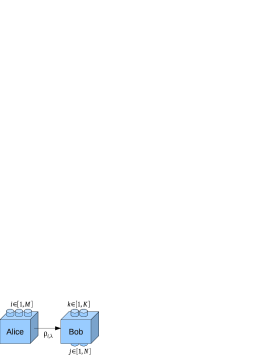
Figure 1: (Color online) Setup for witnessing the dimension of a quantum or classical system. In the most general scenario considered here, Alice and Bob share a hidden random variable $\lambda$. Alice (on the left hand side) owns a preparing device which sends the state $\rho_{i,\lambda}$ to Bob whenever Alice presses button $i\in[1,M]$. Bob owns a measuring device that performs measurement $\Pi_{k,\lambda}$ on the received state whenever Bob presses button $k\in[1,K]$, giving the outcome $j\in[1,N]$.

In the most general scenario, the devices may share a priori correlated information, classical and quantum. However, in many realistic situations, one can assume that the preparing and measuring devices are uncorrelated and that all the correlations observed between the preparation and the measurement are due to the mediating particle connecting the two devices. An intermediate and also valid possibility is to assume that the devices only share classical correlations. In this case, the value of a random variable $\lambda$ distributed according to $q_{\lambda}$ is accessible to preparing and measuring devices. In this work we focus on this last possibility. Alice chooses the value of index $i\in[1,M]$ and sends a fixed state $\rho_{i,\lambda}\in\operatorname{Lin}{\mathcal{H}}$ to Bob. Bob chooses the value of index $k\in[1,K]$ and performs a fixed POVM $\Pi_{k,\lambda}$ on the received state, obtaining outcome $j\in[1,N]$. After repeating the experiment several times (we consider here the asymptotic case), they collect the statistics about indexes $i,j,k$ obtaining the conditional probabilities $p_{j|i,k}$. Note that we also implicitly assume that we are dealing with independent and identically distributed events.

We now introduce the set $\mathcal{Q}$ (the set $\mathcal{C}$) of correlations achievable with quantum (classical) preparations.

Definition 1 (Set of quantum correlations).

For any $M,K,N,d\in\mathbb{N}$ we define the set of quantum correlations $\mathcal{Q}(M,K,N,d)$ as the set of correlations $p_{j|i,k}$ with $i\in[1,M]$, $k\in[1,K]$ and $j\in[1,N]$ such that there exist a Hilbert space $\mathcal{H}$ with $\dim\mathcal{H}=d$, a quantum set $R=\{\rho_{i}\in\operatorname{Lin}\mathcal{H}\}_{1}^{M}$ of states and a set $P=\{\Pi_{k}\}_{1}^{K}$ of POVMs $\Pi_{k}=\{\Pi_{k}^{j}\in\operatorname{Lin}\mathcal{H}\}_{1}^{N}$ for which $p_{j|i,k}=\operatorname{Tr}[\rho_{i}\Pi_{k}^{j}]$, namely

$$\mathcal{Q}:=\{p\;|\; \exists\textrm{ $d$-dimensional Hilbert space }\mathcal{H},$$

$$\exists\textrm{ quantum set }\{\rho_{i}\in\operatorname{Lin}\mathcal{H}\}_{1}^{M}\textrm{ of states},$$

$$\exists\textrm{ set }\{\Pi_{k}\}_{1}^{K}\textrm{ of POVMs }\Pi_{k}=\{\Pi_{k}^{j}\in\operatorname{Lin}\mathcal{H}\}_{1}^{N}$$

$$\textrm{such that }p_{j|i,k}=\operatorname{Tr}[\rho_{i}\Pi_{k}^{j}]\}.$$

Definition 2 (Set of classical correlations).

For any $M,K,N,d\in\mathbb{N}$ we define the set of classical correlations $\mathcal{C}(M,K,N,d)$ as the set of correlations $p_{j|i,k}$ with $i\in[1,M]$, $k\in[1,K]$ and $j\in[1,N]$ such that there exist a Hilbert space $\mathcal{H}$ with $\dim\mathcal{H}=d$, a classical set $R=\{\rho_{i}\in\operatorname{Lin}\mathcal{H}\}_{1}^{M}$ of states and a set $P=\{\Pi_{k}\}_{1}^{K}$ of POVMs $\Pi_{k}=\{\Pi_{k}^{j}\in\operatorname{Lin}\mathcal{H}\}_{1}^{N}$ for which $p_{j|i,k}=\operatorname{Tr}[\rho_{i}\Pi_{k}^{j}]$, namely

$$\mathcal{C}:=\{p\;|\; \exists\textrm{ $d$-dimensional Hilbert space }\mathcal{H},$$

$$\exists\textrm{ classical set }\{\rho_{i}\in\operatorname{Lin}\mathcal{H}\}_{1}^{M}\textrm{ of states},$$

$$\exists\textrm{ set }\{\Pi_{k}\}_{1}^{K}\textrm{ of POVMs }\Pi_{k}=\{\Pi_{k}^{j}\in\operatorname{Lin}\mathcal{H}\}_{1}^{N}$$

$$\textrm{such that }p_{j|i,k}=\operatorname{Tr}[\rho_{i}\Pi_{k}^{j}]\}.$$

We write $\mathcal{Q}$ and $\mathcal{C}$ omitting the parameters $M,K,N,d$ whenever they are clear from the context.

Remark 1.

We notice that, when shared randomness is allowed between quantum (classical) preparations and measurements, the set of achievable correlations is given by $\operatorname{Conv}\mathcal{Q}$ ($\operatorname{Conv}\mathcal{C}$), where for any set $\mathcal{X}$ we denote with $\operatorname{Conv}\mathcal{X}$ the convex hull of $\mathcal{X}$.

The following Lemma shows that it is not restrictive to consider only classical POVMs, that is, measurements consisting of commuting operators, in the definitions of classical correlations.

Lemma 1.

For any correlation $p=\{p_{j|i,k}\}\in\mathcal{C}$ there exist a classical set $R=\{\rho_{i}\}$ of states and a set $Q=\{\Lambda_{k}\}$ of classical POVMs $\Lambda_{k}=\{\Lambda_{k}^{j}\}$ such that $p_{j|i,k}=\operatorname{Tr}[\rho_{i}\Lambda_{k}^{j}]$.

Proof.

By hypothesis there exist a classical set $R=\{\rho_{i}\}$ of states and a set $P=\{\Pi_{k}\}$ of POVMs $\Pi_{k}=\{\Pi_{k}^{j}\}$ such that $p_{j|i,k}=\operatorname{Tr}[\rho_{i}\Pi_{k}^{j}]$ for any $i,j,k$. Take $\Lambda_{k}^{j}=\sum_{i}\langle i|\Pi_{k}^{j}|i\rangle|i\rangle\langle i|$ where $\{|i\rangle\}$ is an orthonormal basis with respect to which the $\rho_{i}$’s are diagonal (it is straightforward to verify that $\Lambda_{k}^{j}\geq 0$ for any $k,j$ and $\sum_{j}\Lambda_{k}^{j}=I$ for any $k$). We have $p_{j|i,k}=\operatorname{Tr}[\rho_{i}\Lambda_{k}^{j}]$ for any $i,j,k$, which proves the statement. ∎

Lemma 1 thus proves that every set of probabilities obtained with commuting states can be performed with classical states and classical POVMs. This clearly implies that commuting states may be equally regarded as classical variables, and commuting-element measurements as read-out of classical variables.

We can now introduce DIDWs. Building only on the knowledge of $p_{j|i,k}$, our task is to provide a lower bound on the dimension $d$ of $\mathcal{H}$

Definition 3.

For any set of correlations $\mathcal{X}$ between $M$ preparations and $K$ measurements with $N$ outcomes, a device independent dimension witness $W_{\mathcal{X}}(p)$ is a function of the conditional probability distribution $p=\{p_{j|i,k}\}$ with $i\in[1,M]$, $k\in[1,K]$, and $j\in[1,N]$ such that

$$W_{\mathcal{X}}(p)>L\Rightarrow p\not\in\mathcal{X},$$ (1)

for some $L$ which depends on $W_{\mathcal{X}}$.

Interestingly, in many situations the value of the bound $L$ in the definition of a dimension witness varies depending on whether one is interested in classical or quantum ensembles of states. This gives a second application for dimension witnesses, namely quantum certification: if the system dimension is assumed, dimension witnesses allow certifying its quantum nature. It is precisely this quantum certification what makes dimension witnesses useful for quantum information protocols PB11 ; HPZGZ11 .

Motivated by Remark 1, for any $M,N,K,d\in\mathbb{N}$ when $\mathcal{X}=\operatorname{Conv}\mathcal{C}(M,N,K,d)$ [when $\mathcal{X}=\operatorname{Conv}\mathcal{Q}(M,N,K,d)$] we say that $W_{\mathcal{X}}(p)$ is a classical (quantum) dimension witness for dimension $d$ in the presence of shared randomness. Given a set $R=\{\rho_{i,\lambda}\}$ of states and a set $P=\{\Pi_{k,\lambda}\}$ of POVMs $\Pi_{k,\lambda}=\{\Pi_{k,\lambda}^{j}\}$, we define $W_{\operatorname{Conv}\mathcal{C}}(R,P):=W_{\operatorname{Conv}\mathcal{C}}(p)$ with $p=\{p_{j|i,k}\}$ and $p_{j|i,k}=\sum_{\lambda}q_{\lambda}\operatorname{Tr}[\rho_{i,\lambda}\Pi_{k,\lambda}^{j}]$, and analogously for $W_{\operatorname{Conv}\mathcal{Q}}$.

In this work we will consider only linear DIDWs, namely inequalities of the form of Eq. (1) such that

$$W(p):=\vec{c}\cdot\vec{p}=\sum_{i,j,k}c_{i,j,k}p_{j|i,k},$$ (2)

where $\vec{c}$ is a constant vector.

Notice that for any function $W(p)$ and constant $L$, the witness $W(p)>L$ is only a representative of a class of equivalent witnesses such that if $W^{\prime}(p)>L^{\prime}$ is a member of the class, then $W(p)>L$ if and only if $W^{\prime}(p)>L^{\prime}$ for any conditional distribution $p$. The following Lemma provides a transformation that preserves this equivalence.

Lemma 2.

Given a function $W(p)=\sum_{i,j,k}c_{i,j,k}p_{j|i,k}$ and a constant $L$, take $W^{\prime}(p)=\sum_{i,j,k}c^{\prime}_{i,j,k}p_{j|i,k}$ with $c^{\prime}_{i,j,k}=c_{i,j,k}+\alpha_{i,k}$ and $L^{\prime}=L+\sum_{i,k}\alpha_{i,k}$ for any $\alpha_{i,k}$ that does not depend on outcome $j$. Then one has $W(p)>L$ if and only if $W^{\prime}(p)>L^{\prime}$ for any $p$.

Proof.

It follows immediately by direct computation. ∎

In the following our task will be to find a set $R$ of quantum states and a set $P$ of POVMs such that a linear witness $W(R,P)$ maximally violates inequality (1). The following Lemma allows us to simplify the optimization problem.

Lemma 3.

The maximum of any linear dimension witness $W(R,P)$ is achieved by an ensemble $R$ of pure states and without shared randomness.

Proof.

The thesis follows immediately from linearity. ∎

Due to Lemma 3 the maximization of Eq. (2) is equivalent to the maximization of

$$W(R,P)=\sum_{i,j,k}c_{i,j,k}\langle\psi_{i}|\Pi_{k}^{j}|\psi_{i}\rangle,$$

over the sets $R=\{\psi_{i}\}$ of pure states and the sets $P=\{\Pi_{k}\}$ of POVMs $\Pi_{k}=\{\Pi_{k}^{j}\}$.

III Properties of the sets of quantum and classical correlations

Before moving to the main results in this article, we discuss in this section several properties of the sets of classical and quantum correlations. In particular, we study whether the sets are convex and prove some inclusions among them. These results allow gaining a better understanding of the geometry of these sets of correlations.

Since classical correlations can always be reproduced by quantum ones, we immediately have $\mathcal{C}\subseteq\mathcal{Q}$ and $\operatorname{Conv}\mathcal{C}\subseteq\operatorname{Conv}\mathcal{Q}$. Moreover, by definition we have $\mathcal{C}\subseteq\operatorname{Conv}\mathcal{C}$ and $\mathcal{Q}\subseteq\operatorname{Conv}\mathcal{Q}$. Here we show an example where $\mathcal{C}$ is non-convex (namely $\mathcal{C}\subset\operatorname{Conv}\mathcal{C}$) and $\mathcal{C}\subset\mathcal{Q}$. Take $M=3$, $K=2$, $N=2$, and $d=2$ in the setup of Figure 1. Consider the following conditional probability distribution $p_{j|i,k}$ of obtaining outcome $j$ on Bob’s device given input $i$ on Alice’s and $k$ on Bob’s

$$p_{j|i,1}=\left(\begin{array}[]{cc}1&0\\ \frac{1}{2}&\frac{1}{2}\\ 0&1\end{array}\right),\qquad p_{j|i,2}=\left(\begin{array}[]{cc}\frac{1}{2}&\frac{1}{2}\\ 1&0\\ \frac{1}{2}&\frac{1}{2}\end{array}\right),$$ (9)

where rows and columns are labeled by $i$ and $j$, respectively.

First we show that $p\in\operatorname{Conv}\mathcal{C}$. Indeed $p$ can be obtained when Alice and Bob share classical correlations represented by a uniformly distributed random variable $\lambda$ taking values $1,2$ making use of the classical set $R=\{\rho_{i,\lambda}\}$ of states and of the set $P=\{\Pi_{k,\lambda}\}$ of classical POVMs $\Pi_{k,\lambda}=\{\Pi_{k,\lambda}^{j}\}$, with

$$\rho_{1,1}=|0\rangle\langle 0|,\quad\rho_{2,1}=|0\rangle\langle 0|,\quad\rho_{3,1}=|1\rangle\langle 1|,$$

$$\rho_{1,2}=|0\rangle\langle 0|,\quad\rho_{2,2}=|1\rangle\langle 1|,\quad\rho_{3,2}=|1\rangle\langle 1|,$$

and

$$\Pi^{1}_{1,1}=|0\rangle\langle 0|,\quad\Pi^{1}_{2,1}=|0\rangle\langle 0|,$$

$$\Pi^{1}_{1,2}=|0\rangle\langle 0|,\quad\Pi^{1}_{2,2}=|1\rangle\langle 1|,$$

which proves that $p=\{p_{j|i,k}=\sum_{\lambda}q_{\lambda}\operatorname{Tr}[\rho_{i,\lambda}\Pi_{k,\lambda}^{j}]\}\in\operatorname{Conv}\mathcal{C}$.

Now we show that $p\in\mathcal{Q}$. Indeed $p$ can be obtained by Alice and Bob making use of the quantum set $R=\{\rho_{i}\}$ of states and of the set $P=\{\Pi_{k}\}$ of quantum POVMs $\Pi_{k}=\{\Pi_{k}^{j}\}$, with

$$\rho_{1}=|0\rangle\langle 0|,\quad\rho_{2}=|+\rangle\langle+|,\quad\rho_{3}=|1\rangle\langle 1|,$$

and

$$\Pi_{1}^{1}=|0\rangle\langle 0|,\quad\Pi_{2}^{1}=|+\rangle\langle+|,$$

which proves that $p\in\mathcal{Q}$.

Finally, we verify that if Alice and Bob make use of classical sets of states and POVMS and do not have access to shared randomness there is no way to achieve the probability distribution $p$ given by Eq. (9). Indeed, to have perfect discrimination between $\rho_{1}$ and $\rho_{3}$ with POVM $\Pi_{1}$ [see Eq. (9)], one must take $\rho_{1}$ and $\rho_{3}$ orthogonal - let us say without loss of generality $\rho_{1}=|0\rangle\langle 0|$ and $\rho_{3}=|1\rangle\langle 1|$, and $\Pi_{1}^{1}=|0\rangle\langle 0|$ and $\Pi_{1}^{2}=|1\rangle\langle 1|$. Due to the hypothesis of classicality of the sets of states, $\rho_{2}$ must be a convex combination of $\rho_{1}$ and $\rho_{3}$. Then, in order to have $p_{j|2,1}$ as in Eq. (9), one has to choose $\rho_{2}=(\rho_{1}+\rho_{3})/2=I/2$. Finally, the only possible choice for $\Pi_{2}$ is $\Pi_{2}^{1}=I$ and $\Pi_{2}^{1}=0$, which is incompatible with the remaining entries of $p_{j|i,2}$ in Eq. (9). This proves that $p\not\in\mathcal{C}$.

The relations between the sets of quantum and classical correlations are schematically depicted in Fig. 2.

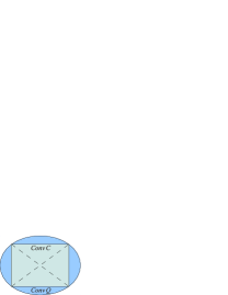
Figure 2: (Color online) Schematic representation of the sets of classical and quantum correlations between preparations, measurements and outcomes. Dashed line represents the (non-convex) set $\mathcal{C}$ of classical correlations without shared randomness; the rectangle represents the set $\operatorname{Conv}\mathcal{C}$ of classical correlations with shared randomness; the ellipsoid represents the set $\operatorname{Conv}\mathcal{Q}$ of quantum correlations with shared randomness.

IV Robustness of dimension witnesses

In practical applications, losses (due to imperfections in the experimental implementations or artificially introduced by a malicious provider) can noticeably affect the effectiveness of dimension witnessing. The main result of this Section is to provide a threshold value for the detection efficiency that allows one to witness the dimension of the systems prepared by a source or to discriminate between its quantum or classical nature.

The task is to determine whether a given conditional probability distribution belongs to a particular convex set, namely $\operatorname{Conv}\mathcal{C}$ or $\operatorname{Conv}\mathcal{Q}$ (see Remark 1). The situation is illustrated in Figure 3.

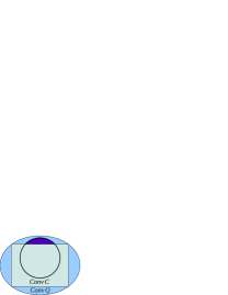
Figure 3: (Color online) The Figure illustrates the problem of the robustness of device independent dimension witness. The convex hulls $\operatorname{Conv}\mathcal{Q}$ and $\operatorname{Conv}\mathcal{C}$ of the sets of quantum and classical correlations are represented as in Figure 2. In the presence of loss, only a subset of the possible correlations is attainable. The subset, surrounded by bold line in the figure, is parametrized by detection efficiency $\eta$. The task is to find the threshold value in $\eta$ such that dimension witnessing is still possible. For example, when the task is to discriminate between the quantum or classical nature of a source, one is interested in achieving correlations in the dark area of the Figure, and our goal is to determine the values of $\eta$ such that this area is not null.

The experimental implementation is constrained to be lossy, namely it can be modeled considering an ideal preparing device followed by a measurement device with non-ideal detection efficiency. This means that any POVM $\Pi_{k,\lambda}$ on Bob’s side is replaced by a POVM $\Pi_{k,\lambda}^{(\eta)}$ with detection efficiency $\eta$, namely

$$\Pi_{k,\lambda}^{(\eta)}:=\{\eta\Pi_{k,\lambda},(1-\eta)I\}.$$ (10)

We notice that each lossy POVM has one outcome more than the ideal one, corresponding to the no-click event. In a general model, the detection efficiency $\eta$ may be different for any POVM $\Pi_{k,\lambda}$. Nevertheless, in the following we assume that they have the same detection efficiency, which is a reasonable assumption if the detectors have the same physical implementation note1 . Analogously given a set $P=\{\Pi_{k,\lambda}\}$ of POVMs we will denote with $P^{(\eta)}=\{\Pi_{k,\lambda}^{(\eta)}\}$ the corresponding set of lossy POVMs. Upon defining $p^{(\eta)}:=\{p_{j|i,k}^{(\eta)}\}$ with $p_{j|i,k}^{(\eta)}=\sum_{\lambda}q_{\lambda}\operatorname{Tr}[\rho_{i,\lambda}\Pi_{k,\lambda}^{j,(\eta)}]$, one clearly has

$$p^{(\eta)}=\eta p^{(1)}+(1-\eta)p^{(0)}.$$ (11)

To attain our task we maximize a given dimension witness over the set of lossy POVMs as given by Eq. (10). Due to the model of loss introduced in Eq. (10) and to the freedom in the normalization of dimension witnesses given by Lemma 2, in the following without loss of generality for any dimension witness $W$ as given in Eq. (2) it is convenient to take

$$c_{i,N,k}=0,\quad\forall i,k.$$ (12)

Then we have the following Lemma.

Lemma 4.

Given a set $R=\{\rho_{i,\lambda}\}_{i=1}^{M}$ of states and a set $P=\{\Pi_{k,\lambda}\}_{k=1}^{K}$ of POVMs $\Pi_{k,\lambda}=\{\Pi_{k,\lambda}^{j}\}_{j=1}^{N-1}$, for any linear dimension witness $W(p)=\sum_{i,j,k}c_{i,j,k}p_{j|i,k}$ with $i\in[1,M]$, $j\in[1,N]$, and $k\in[1,K]$ normalized as in Eq. (12) one has

$$W(R,P^{(\eta)})=\eta W(R,P^{(1)}).$$

Proof.

One has

$$W(R,P^{(\eta)}) =\sum_{i,j,k}c_{i,j,k}\left[\eta p_{j|i,k}^{(1)}+(1-\eta)p_{j|i,k}^{(0)}\right]$$

$$=\eta\,W(R,P^{(1)}),$$

where the first equality follows from Eq. (11) and the second from the fact that $W(p^{(0)})=0$ due to the normalization given in Eq. (12). ∎

In particular from Lemma 4 it follows that for any linear dimension witness $W$ one has

$$\max_{R,P}W(R,P^{(\eta)})=\eta\max_{R,P}W(R,P^{(1)}),$$

$$\arg\max_{R,P}W(R,P^{(\eta)})=\arg\max_{R,P}W(R,P^{(1)}).$$

Due to Lemma 4, it is possible to recast the optimization of dimension witnesses in the presence of loss to the optimization in the ideal case. Then due to Lemma 3 it is not restrictive to carry out the optimization with pure states and no shared randomness. Consider the case where $M=d+1$, $K=d$, and $N=3$. Using the technique discussed in Appendix A one can verify that the witness given by Eq. (2) with the following coefficients

$$c_{i,j,k}=\left\{\begin{array}[]{ll}-1&\textrm{ if }i+k\leq M,\;j=1\\ +1&\textrm{ if }i+k=M+1,\;j=1\\ 0&\textrm{ otherwise}\end{array}\right.,$$ (16)

is the most robust to non-ideal detection efficiency. This fact should not be surprising, as we notice that this witness relies on only $2$ out of $3$ outcomes. According to GBHA10 , we denote it $I_{d+1}$. In GBHA10 (see also Mas02 ) it was conjectured that for any dimension $d$ the dimension witness $I_{d+1}$ is tight in the absence of loss.

Now we provide upper and lower bounds for the maximal value $I_{d+1}^{*}:=\max_{R,P}I_{d+1}$ where the maximization is over any set $R=\{\rho_{i}\in\operatorname{Lin}\mathcal{H}\}$ of states and any set $P=\{\Pi_{k}\}$ of POVMs $\Pi_{k}=\{\Pi_{k}^{j}\in\operatorname{Lin}\mathcal{H}\}$ with $\dim\mathcal{H}=d$.

Lemma 5.

For any dimension $d$ we have $I_{d+1}^{*}\geq I_{d}^{*}+1$.

Proof.

The statement follows from the recursive expression $I_{d+1}=I_{d}+C$, where

$$C:=-\sum_{i=1}^{d}\langle\psi_{i}|\Pi_{1}^{1}|\psi_{i}\rangle+\langle\psi_{d+1}|\Pi_{1}^{1}|\psi_{d+1}\rangle,$$

and noticing that $I_{d}$ and $C$ can be optimized independently. ∎

A tight upper bound for $I_{3}$ was provided in GBHA10 . In the following Lemma we provide a constructive proof suitable for generalization to higher dimensions.

Lemma 6.

For dimension $d=2$ we have $I_{3}^{*}=\sqrt{2}$.

Proof.

The statement follows from standard optimization with Lagrange multipliers method and from the straightforward observation that given two normalized pure states $|v_{0}\rangle$ and $|v_{1}\rangle$, if a pure state $|u\rangle$ can be decomposed as follows

$$|u\rangle=\langle v_{0}|u\rangle|v_{0}\rangle+\langle v_{1}|u\rangle|v_{1}\rangle,$$

then $|\langle v_{0}|u\rangle|=|\langle v_{1}|u\rangle|$. ∎

Making use of Lemmas 5 and 6, we provide upper and lower bounds on $I_{d+1}^{*}$ as follows

$$d-2+\sqrt{2}\leq I_{d+1}^{*}\leq d,$$ (17)

where the second inequality follows from the non discriminability of $d+1$ states in dimension $d$ (see GBHA10 ).

We now make use of these facts to provide our main result, namely a lower threshold for the detection efficiency required to reliably dimension witnessing. We consider the problem of lower bounding the dimension of a system prepared by a non-characterized source in Proposition 1, as well as the problem of discriminating between the quantum or classical nature of a source in Proposition 2.

Proposition 1.

For any $d$ there exists a dimension witnessing setup such that it is possible to discriminate between the quantum and classical nature of a $d$-dimensional system using POVMs with detection efficiency $\eta$ whenever

$$\eta\geq\eta_{qc}:=(d-1)/I_{d+1}.$$ (18)

Furthermore one has

$$\frac{d-1}{d}\leq\eta_{\textrm{qc}}\leq\frac{d-1}{d-2+\sqrt{2}}.$$ (19)

Proof.

We provide a constructive proof of the statement. Take $M=d+1$, $K=d$, and $N=3$, and we show that $I_{d+1}$ satisfies the thesis.

We notice that the maximum value of $I_{d+1}$ attainable with classical states is given by $d-1$ GBHA10 . Then $\eta_{\textrm{qc}}$ is the minimum value of the detection efficiency such that $I_{d+1}$ can discriminate a quantum system from a classical one.

Due to Lemma 4 we have Eq. (18). From Eq. (17) the lower and upper bounds for $\eta_{\textrm{qc}}$ given in Eq. (19) straightforwardly follow. ∎

Notice that $I_{d+1}$ in Eq. (18) can be numerically evaluated with the techniques discussed in Appendix B. Figure 4 plots the value of $\eta_{\textrm{qc}}$ for different values of the dimension $d$ of the Hilbert space $\mathcal{H}$. The threshold in the detection efficiency when $d=2$ is $\eta_{\textrm{qc}}=1/\sqrt{2}$, going asymptotically to $1$ with $d$ as $\sim 1+1/d$.

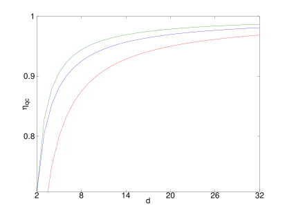
Figure 4: (Color on line) Threshold value (middle line) of the detection efficiency $\eta_{\textrm{qc}}$ as in Eq. (18) as a function of the dimension $d$, obtained through numerical optimization of $I_{d+1}$ with Algorithm 2. The lower bound (lower line) and upper bound (upper line) given by Eq. (19) are also plotted. As expected, the upper bound is tight for $d=2$. The detection efficiency $\eta_{\textrm{qc}}$ asymptotically goes to $1$ as $d\to\infty$ since its upper and lower bound do the same.

Proposition 2.

For any $d$ there exists a dimension witnessing setup such that it is possible to lower bound the dimension of a $d+1$-dimensional system using POVMs with detection efficiency $\eta$ whenever

$$\eta\geq\eta_{\textrm{dim}}:=I_{d+1}/d.$$ (20)

Furthermore one has

$$\eta_{\textrm{dim}}\geq 1-\frac{2-\sqrt{2}}{d}.$$ (21)

Proof.

We provide a constructive proof of the statement. Take $M=d+1$, $K=d$, and $N=3$, and we show that $I_{d+1}$ satisfies the thesis.

We notice that the maximum value of $I_{d+1}$ attainable in any dimension $>d$ is given by $d$ GBHA10 . Then $\eta_{\textrm{dim}}$ is the minimum value of the detection efficiency such that $I_{d+1}$ can lower bound the dimension of a $d+1$ dimensional system.

Due to Lemma 4 we have Eq. (20). From Eq. (17) the lower bound to $\eta_{\textrm{dim}}$ given by Eq. (21) straightforwardly follows. ∎

Notice that $I_{d+1}$ in Eq. (20) can be numerically evaluated with the techniques discussed in Appendix B. Figure 5 plots the value of $\eta_{\textrm{dim}}$ for different values of the dimension $d$ of the Hilbert space $\mathcal{H}$. The threshold in the detection efficiency when $d=2$ is $\eta_{\textrm{qc}}=1/\sqrt{2}$, going asymptotically to $1$ with $d$ as $\sim 1+1/d$. We notice that $\eta_{\textrm{dim}}$ grows faster than $\eta_{qc}$, thus showing that for fixed dimension, the discrimination between the quantum or classical nature of the source is more robust to loss than lower bounding the dimension of the prepared states.

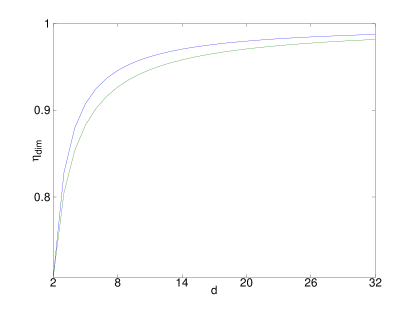
Figure 5: (Color on line) Threshold value (upper line) of the detection efficiency $\eta_{\textrm{dim}}$ as in Eq. (20) as a function of the dimension $d$, obtained through numerical optimization of $I_{d+1}$ with Algorithm 2. The lower bound (lower line) given by Eq. (21) is also plotted. As expected, the lower bound is tight for $d=2$. The detection efficiency $\eta_{\textrm{dim}}$ asymptotically goes to $1$ as $d\to\infty$ since its lower bound does the same (and $\eta_{\textrm{dim}}\leq 1$ is a trivial upper bound).

V Conclusion

In this work we addressed the problem whether a lossy setup can provide a reliable lower bound on the dimension of a classical or quantum system. First we provided some relevant properties of the sets of classical and quantum correlations attainable in a dimension witnessing setup. Then we introduced analytical and numerical tools to address the problem of the robustness of DIDWs, and we provided the amount of loss that can be tolerated in dimension witnessing. The presented results are of relevance for experimental implementations of DIDWs, and can be naturally applied to semi-device independent QKD and QRACs.

We notice that, while we provided analytical proofs of our main results, i.e. Propositions 1 and 2, their optimality as a bound relies on numerical evidences. In particular, they are optimal if the dimension witness $I_{d+1}$ is indeed the most robust to loss for any $d$, which is suggested by numerical evidence obtained with the techniques of Appendix A and Appendix B. Thus, a legitimate question is whether the bounds provided in Propositions 1 and 2 are indeed optimal. Moreover, it is possible to consider models of loss more general than the one considered here, e.g. one in which a different detection efficiency is associated to any POVM.

A natural generalization of the problem of DIDWs, in the ideal as well as in the lossy scenario, is that in the absence of correlations between the preparations and the measurements. In this case, as discussed in this work, the relevant sets of correlations are $\mathcal{Q}$ and $\mathcal{C}$, which are non-convex as shown in Section II. The non convexity of the relevant sets allows the exploitation of non-linear witnesses - as opposed to what we did in the present work. An intriguing but still open question is whether there are situations in which this exploitation allows to dimension witness for any non-null value of the detection efficiency.

Another natural generalization of the problem of DIDWs is that of entangled assisted DIDWs, namely when entanglement is allowed to be shared between the preparing device on Alice’s side and the measuring device on Bob’s side. This problem is similar to that of super-dense coding BW92 . Consider again Fig. 1. In the simplest super-dense coding scenario, Alice presses one button out of $M=4$, while Bob always performs the same POVM ($K=1$) obtaining one out of $N=4$ outcomes. The dimension of the Hilbert space $\mathcal{H}$ is $\dim(\mathcal{H})=2$, but a pair of maximally entangled qubits is shared between the parties. In this case, the results of BW92 imply that a classical system of dimension $4$ (quart) can be sent from Alice to Bob by sending a qubit (corresponding to half of the entangled pair).

Consider the general scenario where now the two parties are allowed to share entangled particles. The super-dense coding protocol automatically ensures that by sending a qubit Alice and Bob can always achieve the same value of any DIDW as attained by a classical quart. Remarkably, the super-dense coding protocol turns out not to be optimal, as we identified more complex protocols beating it. In particular, we found a $(M=4,K=2,N=4)$ situation for which, upon performing unitary operations on her part of the entangled pair and subsequently sending it to Bob, Alice can achieve correlations that can not be reproduced upon sending a quart. This thus proves the existence of communication contexts in which sending half of a maximally entangled pair is a more powerful resource than a classical quart. This observation is analogous to that done in PZ10 , where it was shown that entangled assisted QRACs (where an entangled pair of qubits is shared between the parties) outperform the best of known QRACs. For these reasons we believe that the problem of entangled assisted DIDWs deserves further investigation.

Appendix A Numerical optimization of dimension witnesses

Given a linear dimension witness $W$ the following algorithm converges to a local maximum of $W(R,P)$.

Algorithm 1.

For any set $R^{(0)}=\{\psi_{i}^{(0)}\}$ of pure states and any set $P^{(0)}=\{\Pi_{k}^{(0)}\}$ of POVMs $\Pi_{k}^{(0)}=\{\Pi_{k}^{j,(0)}\}$,

1. let $|\bar{\psi}_{i}^{(n+1)}\rangle=\left[(1-\epsilon)I+\epsilon\sum_{j,k}c_{i,j,k}\Pi_{k}^{j,(n)}\right]|\psi_{i}^{(n)}\rangle$,

2. let $\bar{\Pi}_{k}^{j,(n+1)}=\left\{\left[(1-\epsilon)I+\epsilon\sum_{i}c_{i,j,k}\psi_{i}^{(n)}\right]\sqrt{\Pi_{k}^{j,(n)}}\right\}^{2}$,

3. normalize $|\psi_{i}^{(n+1)}\rangle=||\bar{\psi}_{i}^{(n+1)}||^{-1/2}|\bar{\psi}_{i}^{(n+1)}\rangle$,

4. normalize $\Pi_{k}^{j,(n+1)}=S_{k}^{-\frac{1}{2}}\bar{\Pi}_{k}^{j,(n+1)}S_{k}^{-\frac{1}{2}}$ with $S_{k}=\sum_{j}\bar{\Pi}_{k}^{j,(n+1)}$.

As for all steepest-ascent algorithm, there is no protection against the possibility of convergence toward a local, rather than a global, maximum. Hence one should run the algorithm for different initial ensembles in order to get some confidence that the observed maximum is the global maximum (although this can never be guaranteed with certainty). Any initial set of states and any initial set of POVMs can be used as a starting point, except for a subset corresponding to minima of $W(R,P)$. These minima are unstable fix-points of the iteration, so even small perturbations let the iteration converge to some maxima. The parameter $\epsilon$ controls the length of each iterative step, so for $\epsilon$ too large, an overshooting can occur. This can be kept under control by evaluating $W(R,P)$ at the end of each step: if it decreases instead of increasing, we are warned that we have taken $\epsilon$ too large.

Referring to Fig. 1, the simplest non-trivial scenario one can consider is the one with $M=3$ preparations and $K=2$ POVMs each with $N=3$ outcomes, one of which corresponding to no-click event. In this case one has several tight classical DIDWs. Applying Algorithm 1 we verified that among them the most robust to loss is given by Eq. (2) with coefficients given by Eq. (16).

Appendix B Numerical optimization of $I_{d+1}$

The following Lemma proves that the POVMs maximizing $I_{d+1}$ for any dimension $d$ are such that one of their elements is a projector on a pure state, thus generalizing a result from Mas05 .

Lemma 7.

For any dimension $d$, the maximum of $I_{d+1}$ is achieved by a set $P=\{\Pi_{k}\}$ of POVMs $\Pi_{k}=\{\Pi_{k}^{j}\}$ with $\Pi_{k}^{1}$ a projector with $\operatorname{rank}\Pi_{k}^{1}=1$ for any $k$.

Proof.

For any fixed set $R=\{\psi_{i}\}$ of pure states define $A_{k}:=-\sum_{i\neq k}\psi_{i}$, $B:=\psi_{k}$, and $X_{k}:=A_{k}+B_{k}$. Then clearly $A_{k}\leq 0$, $B_{k}\geq 0$ and $\operatorname{rank}B_{k}=1$ for any $k$. From Eq. (2) it follows immediately that the optimal set $P^{*}=\{\Pi_{k}^{*}\}$ of POVMs $\Pi_{k}^{*}=\{\Pi^{*j}_{k}\}$ is such that $\Pi_{k}^{*1}=\arg\min_{\Pi_{k}^{1}}\operatorname{Tr}[X\Pi_{k}^{1}]$. The optimum of $I_{d+1}$ is achieved when $\Pi_{k}^{1}$ is the sum of the eigenvectors of $X_{k}$ corresponding to positive eigenvalues.

Upon denoting with $\lambda_{1}(A_{k})\geq\dots\geq\lambda_{n}(A_{k})$ the eigenvalues of $A_{k}$, the Weyl inequality (see for example Bha06 ) $\lambda_{1}(X_{k})\leq\lambda_{1}(A_{k})+\lambda_{n}(B_{k})$ holds for any $n$. Since $\lambda_{1}(A_{k})\leq 0$ and $\lambda_{n}(B_{k})=0$ for any $k$ and for any $n\neq 0$, the thesis follows immediately. ∎

Algorithm 1 can be simplified using Lemma 7. The following algorithm converges to a local maximum of $I_{d+1}$.

Algorithm 2.

For any set $R^{(0)}=\{\psi_{i}^{(0)}\}$ of pure states and any set $P^{(0)}=\{\Pi_{k}^{(0)}\}$ of POVMs $\Pi_{k}^{(0)}=\{\Pi_{k}^{j,(0)}\}$,

1. let $|\bar{\psi}_{i}^{(n+1)}\rangle=|\psi_{i}^{(n)}\rangle+\epsilon\sum_{j,k}c_{i,j,k}\langle\pi_{k}^{(n)}|\psi_{i}^{(n)}\rangle|\pi_{k}^{(n)}\rangle$,

2. let $|\bar{\pi}_{k}^{(n+1)}\rangle=|\pi_{k}^{(n)}\rangle+\epsilon\sum_{i,k}c_{i,j,k}\langle\psi_{i}^{(n)}|\pi_{k}^{(n)}\rangle|\psi_{i}^{(n)}\rangle$,

3. normalize $|\psi_{i}^{(n+1)}\rangle=||\bar{\psi}_{i}^{(n+1)}||^{-1/2}|\bar{\psi}_{i}^{(n+1)}\rangle$,

4. normalize $|\pi_{k}^{(n+1)}\rangle=||\bar{\pi}_{k}^{(n+1)}||^{-1/2}|\bar{\pi}_{k}^{(n+1)}\rangle$.

The same remarks made about Algorithm 1 hold true for Algorithm 2. Nevertheless, we verified that in practical applications Algorithm 2 always seems to converge to a global, not a local maximum. This can be explained considering that without loss of generality it optimizes over a smaller set of POVMs when compared to Algorithm 1. Moreover, we noticed that the optimal sets of states and POVMs are real, namely there exists a basis with respect to which states and POVM elements have all real matrix entries. A similar observation was done in FFW11 in the context of Bell’s inequalities.

References

- (1) N. Brunner, S. Pironio, A. Acín, N. Gisin, A. A. Méthot, and V. Scarani, Phys. Rev. Lett. 100, 210503 (2008).
- (2) S. Wehner, M. Christandl, and A. C. Doherty, Phys. Rev. A 78, 062112 (2008).
- (3) M. M. Wolf and D. Perez-García, Phys. Rev. Lett. 102, 190504 (2009).
- (4) R. Gallego, N. Brunner, C. Hadley, and A. Acín, Phys. Rev. Lett. 105, 230501 (2010).
- (5) M. Hendrych, R. Gallego, M. Mičuda, N. Brunner, A. Acín, and J. P. Torres, Nature Phys. 8, 588-591 (2012).
- (6) H. Ahrens, P. Badzia̧g, A. Cabello, and M. Bourennane, arXiv:quant-ph/1111.1277.
- (7) M. Pawłowski and N. Brunner, Phys. Rev. A 84, 010302 (2011).
- (8) H.-W. Li, M. Pawłowski, Z.-Q. Yin, G.-C. Guo, and Z.-F. Han, arxiv:quant-ph/1109.5259.
- (9) M. Pawłowski and M. Żukowski, Phys. Rev. A 81, 042326 (2010).
- (10) I. L. Chuang and M. A. Nielsen, Quantum Information and Communication (Cambridge, Cambridge University Press, 2000).
- (11) This is not the case in the hybrid scenario where different types of detectors (e.g. photodetectors and homodyne measurements) are used. A similar scenario was proposed for example in the context of Bell inequalities CBSSS11 .
- (12) D. Cavalcanti, N. Brunner, P. Skrzypczyk, A. Salles, V. Scarani, Phys. Rev. A 84, 022105 (2011).
- (13) Ll. Masanes, arXiv:quant-ph/0210073
- (14) C. H. Bennett and S. J. Wiesner, Phys. Rev. Lett. 69, 2881 (1992).
- (15) Ll. Masanes, arXiv:quant-ph/0512100.
- (16) R. Bhatia, Positive Definite Matrices (Princeton University Press, Princeton, 2006).
- (17) T. Franz, F. Furrer, and R. F. Werner, Phys. Rev. Lett. 106, 250502 (2011).